Target soybean leaf automatic segmentation based on object detection and interactive segmentation models

Plant phenotype plays an important role in crop breeding and planting. Leaf phenotype is an important part of plant phenotype. In order to analyze the leaf phenotype, the target leaf is required to be segmented from the complex background image. In this paper, an automatic soybean leaf segmentation method based on object detection and interactive segmentation models is proposed. Firstly, the Libra R-CNN object detection algorithm is used to detect all soybean leaves in the image. Then, based on the idea that the target soybean leaf is located in the center of the image and the area is large, the detection bounding box of the target leaf is selected. In order not to destroy the segmentation result, the bounding box is optimized to completely enclose the whole leaf. Finally, according to the optimized bounding box, the prior channels of foreground and background are constructed using Gaussian model. The two channels together with the original image are as the input of the interactive object segmentation with inside-outside guidance model to segment the target soybean leaf. A large number of qualitative and quantitative experimental results show that the method has high segmentation accuracy and strong generalization capacity.

Keywords:

Subject: Computer Science and Mathematics - Computer Vision and Graphics

1. Introduction

The study of soybean leaf phenotype plays an important role in breeding new soybean varieties, real-time monitoring of soybean plant growth, and refined cultivation management (Reynolds et al., 2020). The phenotype parameters of soybean leaf include leaf length, leaf width, leaf area, etc. To obtain these data, traditional methods rely on manual measurement, which is time-consuming and causes irreversible damage to crops (Yang et al., 2020). To avoid damaging plant growth, data collection in a non-contact manner is gradually becoming a trend (ward et al., 2019). Images, as the most convenient and easily accessible medium, have become the main data type. The target leaf image for phenotype parameter measurement usually contain complex backgrounds when collecting under the growth state of soybean plants. The background contains leaves with the same color and texture as the target leaves, which brings difficulty to segment the target leaves.

Fast and accurate leaf image segmentation under complex background conditions is always a difficult problem. Many traditional techniques have been adopted to solve the issue (Kumar and Domnic, 2019; Bai et al., 2017; Tian et al., 2019; Gao and Lin, 2018). Those techniques often heavily rely on initial parameters, which limits the application. In recent years, deep learning based segmentation models for crop are widely developed. Bhagat et al. constructed a leaf segmentation network with an encoder-decoder structure, where EfficientNet-B4 is as an encoder and a lateral output structure is introduced to improve segmentation accuracy (Bhagat et al., 2022). Wang et al. proposed an automated maize leaf segmentation algorithm and utilized image restoration technique to improve the segmentation results (Wang et al.,2020). Liu et al. combined Mask R-CNN with DBSCAN clustering algorithm to produce an accurate segmentation result (He et al., 2017; Liu et al., 2020). Tian et al. designed an improved Mask R-CNN model by combining Mask R-CNN’s mask prediction branch with the U-Net model to improve the segmentation accuracy for apple blossom images (Tian et al., 2020). All those methods are applied to simple scenarios. For complex images, Wang et al. proposed a DUNet model, which first removed the complex background using DeepLabv3 (Chen et al., 2018) and then segmented the leaf lesion spots using the UNet (Ronneberger et al., 2015) model (Wang et al., 2021).Tassis et al. proposed a two-stage model by identifying the target leaf region first with Mask R-CNN, and then segmenting the leaf lesion region with the UNet model (Tassis et al., 2021). Our model also includes two-stage of object detection and target object segmentation. However, a more difficult problem of segmenting target leaf from multiple similar leaves is given.

Object detection model is mainly divided into single stage and two-stage detectors. YOLO (Redmon et al., 2016; Redmon et al., 2017) and SSD (Liu et al., 2016; Chandio et al., 2022) are single stage detectors. They are simpler and faster than two-stage detectors, but their accuracy is relatively weak. R-CNN (Girshick et al., 2014) introduced a two-stage detector for the first time. The followed Fast RCNN (Girshick, 2015) and Fast R-CNN (Ren et al., 2015) promoted the development. Faster R-CNN proposed a region proposal network and adopted an end-to-end training approach. Cascade R-CNN extended Faster R-CNN to a multi-stage detector (Cai and Vasconcelos, 2018). Mask R-CNN extended Faster RCNN by adding a mask branch (He et al., 2017). Oriented R-CNN (xie et al., 2021) generated high-quality oriented candidate boxes. This paper adopted Libra R-CNN (Pang et al., 2019) which obtains better detection accuracy by optimizing sampling, feature fusion and Loss function definition.

We adopt interactive segmentation model to segment target leaf, which can provide prior information. GrabCut uses bounding boxes to guide the segmentation process, which is one of the pioneering works of interactive segmentation tasks (Rother et al., 2004). Similarly, Xu et al. also uses bounding boxes as input to generate a two-dimensional distance map, and then segments the objects within the box using an encoder and decoder network model (Xu et al., 2017). IFCN guides users to click on positive (foreground) and negative (background) points for interactive segmentation based on the automatic segmentation model (Xu et al., 2016; Long et al., 2015). proposed a DEXTR segmentation model using four extreme points (Maninis et al., 2018). When the interactive click meets the conditions of multiple objects, Li et al. provided a solution to select the optimal result (Li et al., 2018). Song et al. proposed an interactive image segmentation method based on reinforcement learning to simplify user interaction (Song et al., 2018). Benenson et al. proposed a two-stage interactive segmentation method by combining bounding box and click two interaction modes (Benenson et al., 2019). First a coarse result is obtained according to bounding box, and then the fine result is generated by utilizing click. Lin et al. proposed that the first point generally represents global information, while the subsequent points are all local (Lin et al., 2020). Different weights are assigned to the first point to achieve better segmentation results. The paper chooses interactive object segmentation with inside-outside guidance model proposed by Zhang et al. due to its convenient interaction and ideal result for our problem (Zhang et al., 2020).

This paper presents a target soybean leaf segmentation model. First, all soybean leaves in the image are detected using object detection algorithm. Then the target soybean leaf is located based on the idea that the target soybean leaf is in the central position of the image and occupies a large image region. Finally, the target background and foreground priors are provided according to the bounding box of target soybean leaf and they guide the segmentation model to obtain accurate target soybean leaf. The contributions of this research can be summarized as follows: 1) An automatic target soybean leaf segmentation model was designed, and the results of qualitative and quantitative analysis showed that the model achieved satisfactory segmentation effect. 2) An accurate target soybean leaf location algorithm based on the leaf position and size is provided. And a localization accuracy driven parameter setting is designed to balance the importance of position and size. 3) A segmentation accuracy guided tolerance offset distance is proposed for optimizing the leaf bounding box. Multiple offset strategies to adjust the vertex positions of target bounding box are designed to handle the fluctuation of the segmentation accuracy. The scheme to achieve the maximize segmentation accuracy is selected.

2. Materials and Methods

2.1. Data Set Acquisition

The soybean leaf images used were taken in an experimental soybean cultivation field. We performed cropping and image enhancement operations on the collected images and scaled them to a uniform resolution of 512×512. Totally, we acquired 2954 images to construct data set, dividing 1619 images for model training and 1335 for model evaluation. Figure 1 shows samples of the leaf images in data set.

Figure 1. Soybean leaf samples in data set.

For leaf detection and segmentation model based on deep learning, training set is required. The quality of training set tends to affect the prediction accuracy of the model. The leaf detection and segmentation networks in our model are both supervised and the training data need to be annotated. For images with multiple similar objects, it is necessary to annotate all objects to improve detection accuracy. Labelme is a commonly used free and open source annotation software for data annotation. Therefore, we utilized Labelme to label all the salient leaves in the leaf images based on the idea that the target leaf is also salient. The labelled samples for leaf detection model are shown in Figure 2a. The goal of the leaf segmentation network is to segment the target leaf. So when constructing the training set, we only need to label the mask of the target leaf in the image, as shown in Figure 2b.

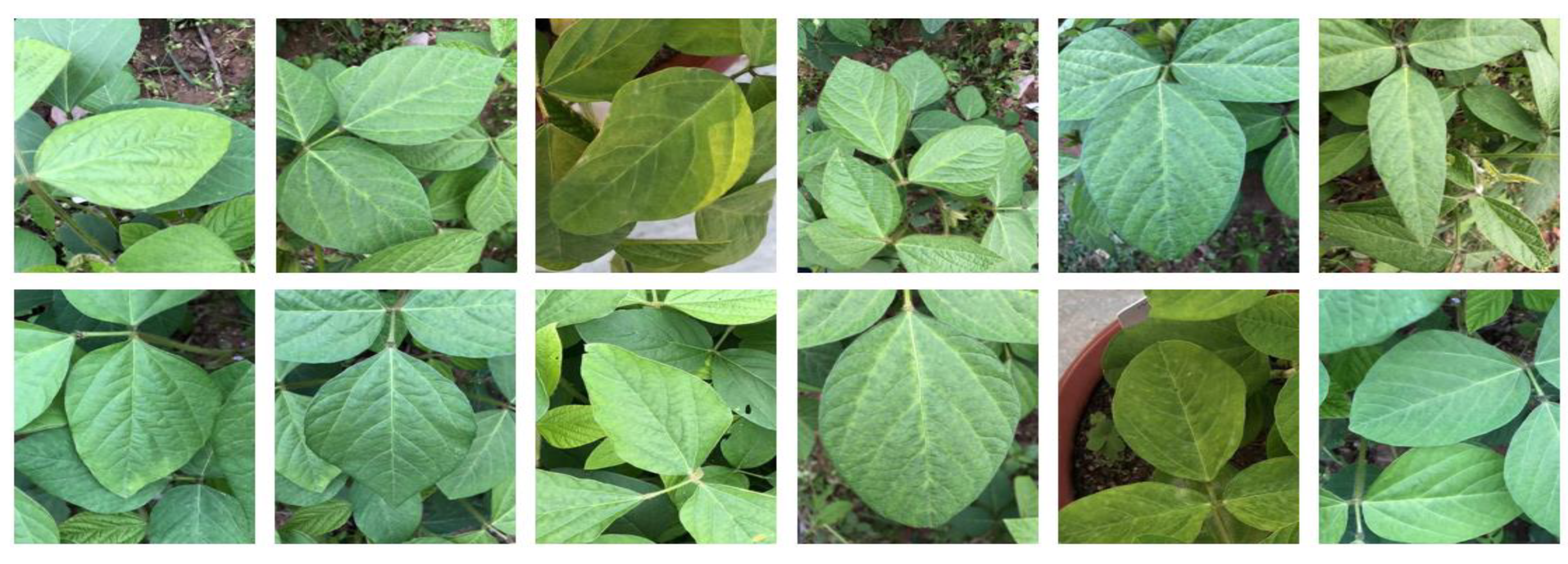
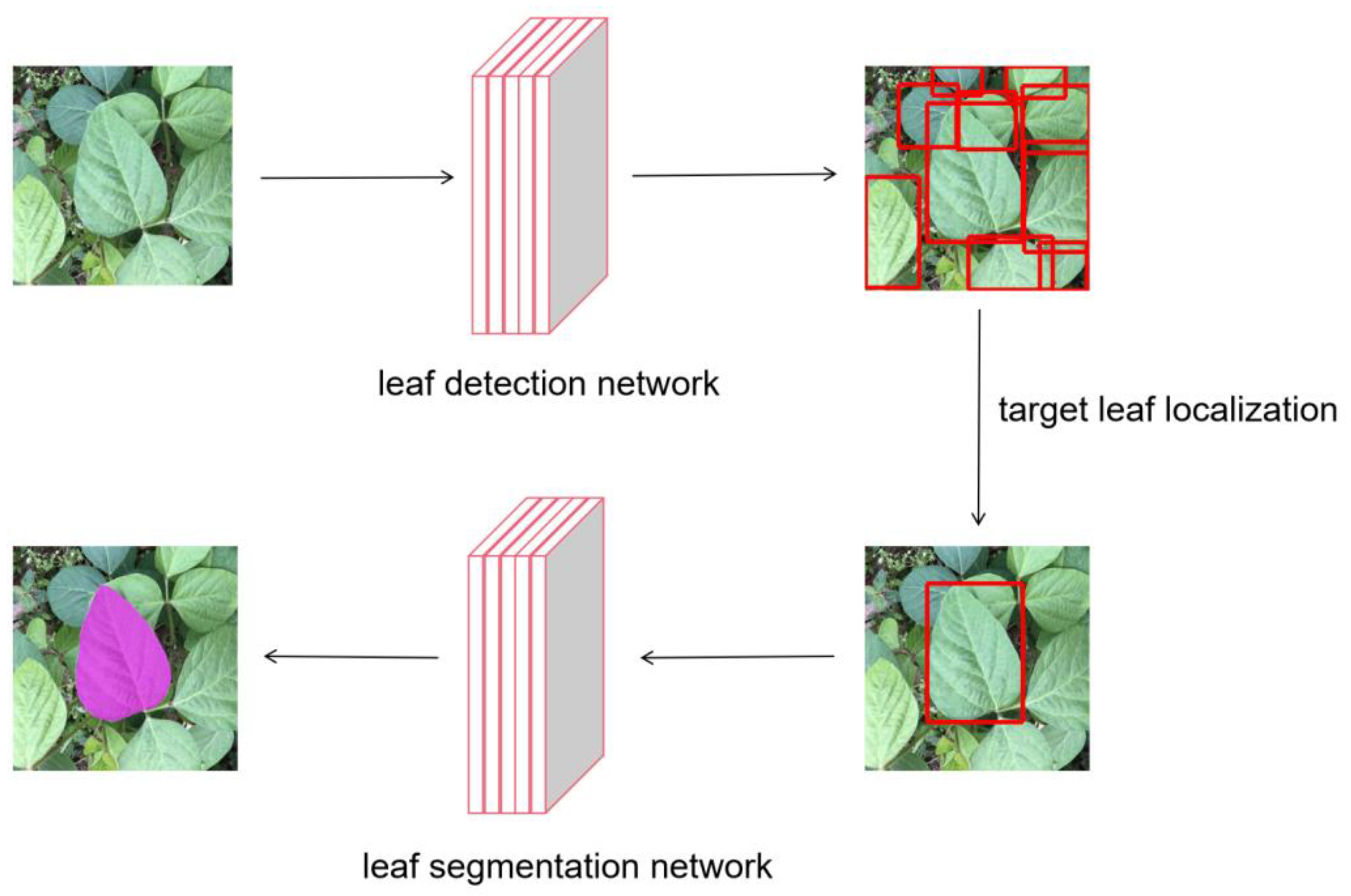
2.2. Methods

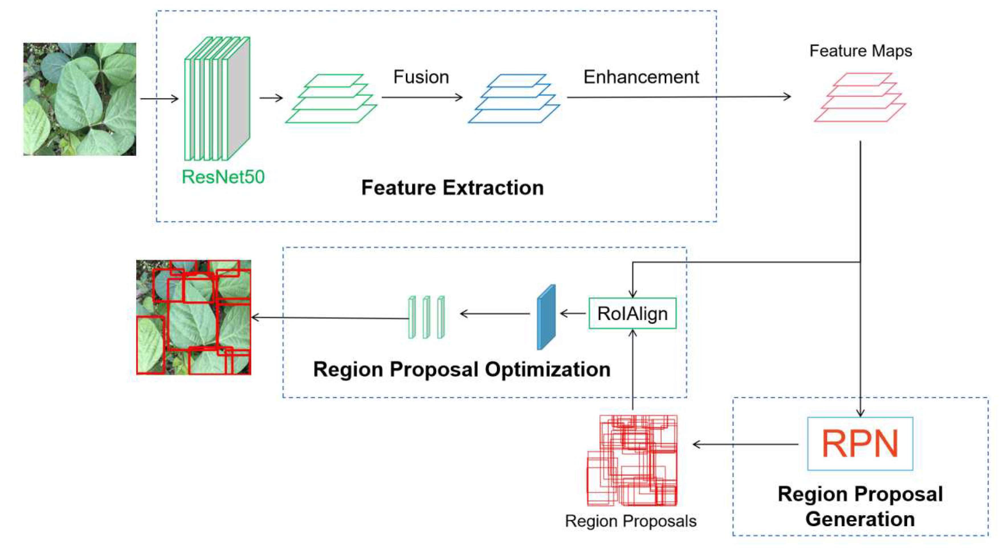
A soybean leaf image segmentation model is proposed and the pipeline is shown in Figure 3. Firstly, the image is input into the leaf detection network named as Libra R-CNN, which predicts all possible leaf bounding boxes in the image. Secondly, the leaf with the larger leaf bounding box and closer to the center of the image is selected as target leaf. Finally, the target leaf, together with its bounding box, is input into the bootstrap segmentation network. The output is the segmentation of the target leaf.

2.2.1. Libra R-CNN Network for Leaf Detection

The overall architecture of leaf detection model uses Libra R-CNN network, which is composed of feature extraction, region proposal generation and region proposal optimization, as shown in Figure 4. Firstly, feature extraction is performed on the input image. In this phase, the feature maps of different layers are fused and enhanced. Secondly, a large number of region proposals are generated on the basis of the output feature maps. Finally, the final prediction results are obtained by optimizing the region proposals.

a) Feature extraction for leaf detection

The feature extraction module includes basic feature extraction, feature fusion and feature enhancement, and its overall structure is shown in Figure 5. Basic feature extraction uses the residual neural network (ResNet) (He et al., 2016), which shows strong feature extraction ability and is widely used in the feature extraction module of various deep neural networks. Feature maps of four different sizes are built from bottom to top. A pyramid structure of feature maps is constructed by using the forward propagation of convolutional neural networks to obtain feature maps of different size. The size between two neighbor feature maps with different resolutions is twice.

Feature fusion follows basic feature extraction. In convolutional networks, the low-level feature map has less semantic information, and the target location is relatively accurate. The high-level feature map has more semantic information, and the target location is rough. Feature fusion combines low-level and high-level features to fully utilize the features of each level, thereby better capturing image details and contextual information. Feature pyramid network (FPN) (Lin et al., 2017) is adopted for feature fusion. The feature maps output {B2, B3, B4, B5} from the last layer of each stage in ResNet50 except the first stage are used to construct the feature map pyramid. First double upsampling is performed on B5 to achieve the same resolution as B4. At the same time, 1x1 convolution is operated on B4 to get the same channel numbers as the upsampling feature maps of B5. Then add them together element by element to obtain the new feature map as C4. And so on to get feature maps C3 and C2, as shown in Figure 5. So the features are continuously fused.

Feature enhancement is given after feature fusion. Multi-level features are further strengthened using the same deeply integrated balanced semantic features. First, the multi-level features {C2, C3, C4, C5} is scaled to the same size such as C4 with interpolation (C5) or max-pooling (C2 and C3) operation respectively. Set the resized features as {C2, C3, C4, C5}, the average feature is calculated as

C = \frac{1}{4} \sum_{i = 2}^{5} C_{i}

(1)

Then the average feature is further refined to be more discriminative by embedded Gaussian non-local attention (Wang et al., 2018). That is, for feature

x_{i}

in position

i

and feature

x_{j}

in any position

j

in average feature C, the attention is defined as

y_{i} = \frac{1}{\sum_{\forall j} e^{{θ (x_{i})}^{T} ϕ (x_{j})}} \sum_{\forall j} e^{{θ (x_{i})}^{T} ϕ (x_{j})} g (x_{j})

(2)

where

θ, ϕ

and

g

are 1*1 convolution operator.

With the attention as residual block, feature

r_{i}

in position

i

in the refined average feature R is written as

r_{i} = W_{r} y_{i} + x_{i}

(3)

where

W_{r}

is convolution operation with the same channel number as

x

The refined average feature R is as the integrated balanced semantic features. Feature R is then rescaled to the same resolutions as {C2, C3, C4, C5} and is added with them separately to form new multi-scale features {P2, P3, P4, P5} to strengthen the features. The features {P2, P3, P4, P5} are used for leaf detection.

b) Region proposal generation

The region proposal generation is including three steps, as shown in Figure 6. First, according to input image size and feature maps, the anchor generator generates thousands of anchors. Second, IoU-balanced sampling is executed on the anchors to select. Third, with the selected anchors and feature maps as the input, region proposal generator generates region proposals.

The anchors are generated based on the feature maps. Specifically, for each feature point of one feature map, three anchors are generated on the corresponding image position. The anchors are with the same area and three different aspect ratios of 1:1, 1:2 and 2:1, as shown in Figure 7. We assign the anchor size of 1:1 aspect ratio for feature map P2 to be 13*13. Since deeper feature map has a wider field of perception and can better detect large-sized objects, the anchors mapped to the original image are assigned a larger size. According to the scale factors between the sizes of feature maps, the anchor sizes of 1:1 aspect ratio for feature map P3, P4 and P5 are 25*25, 50*50 and 100*100 separately.

The traditional random sampling method ignores large number of hard samples, which can improve the accuracy of the network. IoU-balanced Sampling is adopted to mine hard anchor samples. IoU(Intersection over Union) is the ratio of the overlap area and the union area between the predicted bounding box and the ground truth, which is defined as

I o U = \frac{A r e a o f O v e r l a p}{A r e a o f U n i o n}

(4)

If an anchor has an IoU value less than 0.3, it is classified as a negative sample. If the IoU value is greater than 0.7, it is classified as a positive sample. In other cases, anchors are classified as discarded samples and do not participate in the loss calculation. IoU-balanced Sampling uses stratified sampling to select hard negative samples. This is done by dividing the sampling interval equally into K bins according to the IoU, and then selecting samples from them uniformly.

The region proposal generator generates the region proposals. First, the class (foreground or background) and regression parameters (the position, length and width) are predicted for each anchor. Then proposals are generated according to the regression parameters. Finally, region proposals are obtained by non-maximum suppression (NMS) which searches for proposals with the highest prediction probability in the local area.

c) Region proposal optimization

Region proposal optimization is the process of adjusting the position, width and height of region proposals and predicting the probability scores of each box for all classes. The network structure is shown in Figure 8. First, RoIAlign converts features of RoI (region of interest) to a small feature map with a fixed size of 77. RoIAlign, proposed by Mask R-CNN, is a feature extraction module for RoIs. It maps the region proposals to the corresponding feature map to obtain RoIs and then performs a maximum pooling operation on thses specific regions to produce 77 feature matrices. To pool the specific region, a bilinear interpolation is used to calculate each element value of the matrices. Second, these 77 feature matrices are flattened and inputed into two serial fully connected layers. Then two parallel branches of the fully connected layer are followed, which output the class probabilities and regression parameters for each proposal separately. Finally, the regression parameters are used to correct the position and size of the proposals. A series of leaf bounding boxes can be obtained by selecting the boxes with high leaf class probability.

d) Loss function definition for leaf detection

The loss of the leaf detection network consists of two parts, one for the RPN and the other for the region proposal optimization network, which is defined as

L = L_{r p n} + L_{r p o}

(5)

The loss function

L_{r p n}

for the RPN network is given as

L_{r p n} = \frac{1}{N_{c l s}} \sum_{i} L_{c l s} (p_{i}, p_{i}^{*}) + \frac{1}{N_{r e g}} \sum_{i} p_{i}^{*} L_{r e g} (t_{i}, t_{i}^{*})

(6)

which includes the classification loss

L_{c l s}

and the regression loss

L_{r e g}

of anchors, where

p_{i}

is the probability that anchor i is predicted to be positive.

p_{i}^{*}

is 1 if anchor

i

is positive and 0 otherwise.

t_{i}

is the four predicted regression parameters on anchor

i

, while

t_{i}^{*}

is the actual regression parameters. The anchor classification loss

L_{c l s}

defined by binary cross-entropy is

L_{c l s} = - [p_{i}^{*} l o g (p_{i}) + (1 - p_{i}^{*}) l o g (1 - p_{i})

(7)

the regression loss

L_{r e g}

is based on balanced L1 loss. The key idea of balanced L1 loss is suppressing the regression gradients from outliers (inaccurate samples) to balance the involved samples and tasks. The gradient function for

L 1_{b a l a n c e d} (x)

is given as

\frac{\partial {L 1}_{b a l a n c e d (x)}}{\partial_{x}} = \{\begin{matrix} α \ln (b | x | + 1) i f | x | < 1 \\ γ o t h e r w i s e \end{matrix}

(8)

where

α

and b are control factors,

γ

is a constant. To ensure continuity of the gradient, set

α \ln (b + 1) = γ

. In our experiments,

α

is set to 0.5 and

γ

is set to 1.5.

The balanced L1 loss is got by integrating the gradient formulation in Equation (8) as

L 1_{b a l a n c e d} (x) = {\begin{matrix} \frac{α}{b} (b | x | + 1) l n (b | x | + 1) - α | x | & i f | x | < 1 \\ γ | x | + C & o t h e r w i s e \end{matrix}

(9)

where C is a constant.

The definition of regression loss

L_{r e g}

using Balanced L1 Loss is

L_{r e g} (t_{i}, t_{i}^{*}) = \sum_{j \in {x, y, w, h}} L 1_{b a l a n c e d} (t_{i j} - t_{i j}^{*})

(10)

where

t_{i j}

(j=x, y, w, h) is a specific regression parameter of

t_{i}

, which is used to correct the x-coordinate, y-coordinate, height and width of Anchor respectively, and

t_{i j}^{*}

is a specific regression parameter of

t_{i}^{*}

. The loss of leaf bounding box prediction network

L_{b p n}

is defined as

L_{r p o} = - \sum_{i} L_{c l s 1} (p_{i}^{^{'}}, u_{i}) + \frac{1}{N_{c l s}^{^{'}}} \sum_{i} [u_{i} > 0] L_{r e g} (t_{i}^{u_{i}}, v_{i})

(11)

Here

p_{i}^{^{'}}

is the softmax probability of proposal

i

for each category (including background).

u_{i}

is the actual category label.

t_{i}^{u_{i}}

is the predicted regression parameters for the category

u_{i}

corresponding to proposal

i

and

v_{i}

is the actual regression parameters. The classification loss

L_{c l s 1}

of the proposals is defined using the cross-entropy loss for multiple classifications as

L_{c l s 1} (p_{i}^{^{'}}, u_{i}) = - l o g (p_{i}^{u_{i}})

(12)

where

p_{i}^{u_{i}}

is the predicted probability of the category

u_{i}

corresponding to proposal

i

. In this study, although

L_{c l s}

and

L_{c l s 1}

are used for different purposes, one for binary classification and the other for multiple classification, since the leaf bounding box prediction network predicts only two category probabilities for a proposal: background and leaf,

L_{c l s 1}

here is equal to

L_{c l s}

. The regression loss

L_{r e g}

is used to defined the regression loss of Proposals, which is calculated in equation (10).

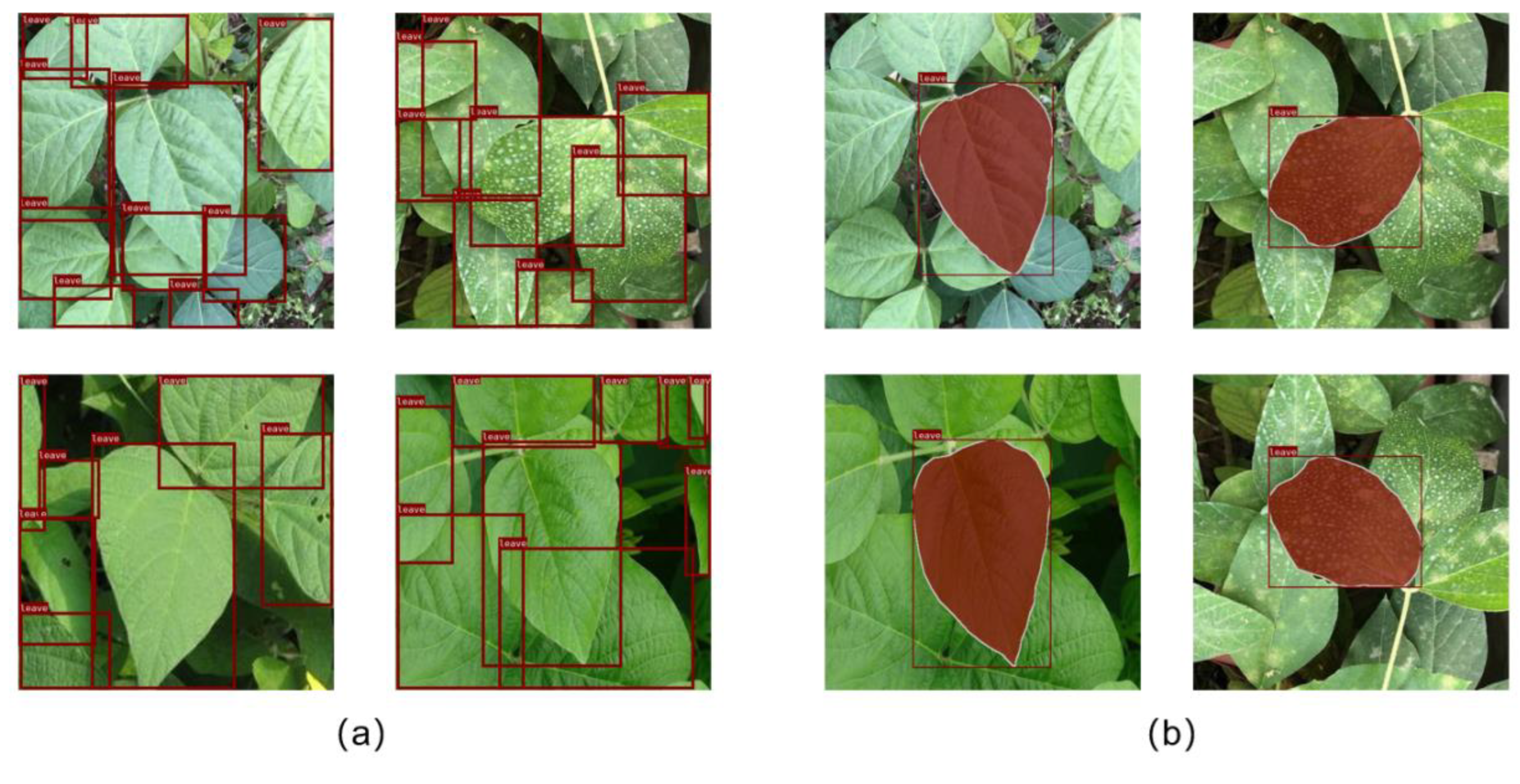
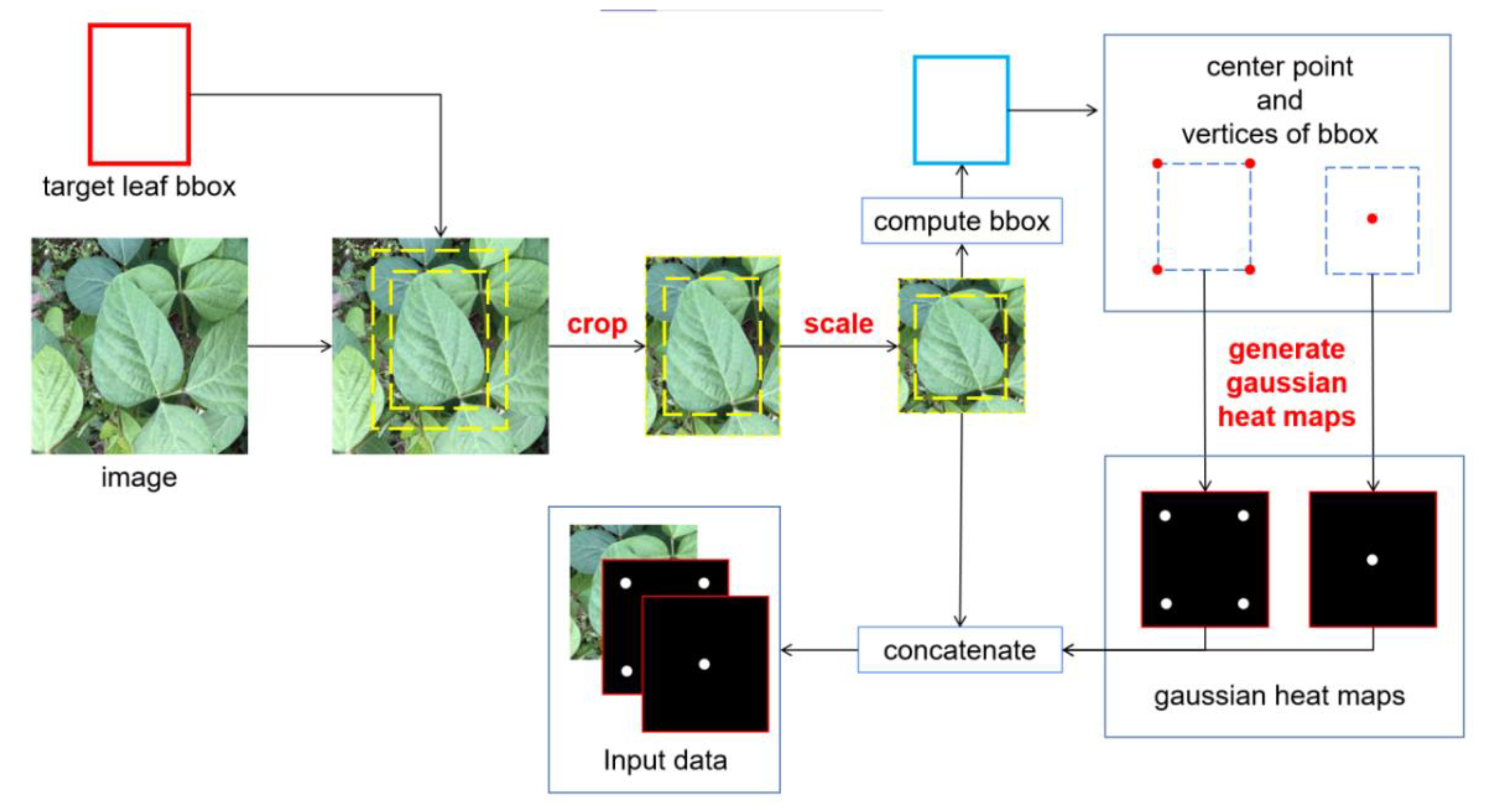
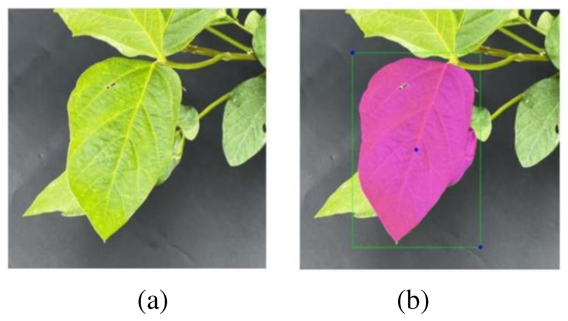
2.2.2. Target Leaf Localization

We have detected the rectangular bounding boxes of all possible leaves in the image during the detection phase. However, only the leaf is needed which is located in the central region of the image and with a large size, so is the bounding box. The distance between the two center points of the image and each rectangular bounding box is used to measure the position, which is defined as

d_{i} = \sqrt{{(p_{i} (x) - c (x))}^{2} + {(p_{i} (y) - c (y))}^{2}}

(13)

where

p_{i}

is the center position of the i-th rectangular bounding box and c is the center position of the image. We normalize the distance as

d_{n i} = \frac{d_{i} - d_{m i n}}{d_{m a x} - d_{m i n}}

(14)

where

d_{m a x} = m a x {d_{i}}

and

d_{m i n} = m i n {d_{i}}

, that is,

d_{m a x}

and

d_{m i n}

is the maximum distance and the minimum distance of all

d_{i}

Similarly, set the area of the i-th rectangular bounding box

S_{i}

, the maximum area and the minimum area of all bounding boxes

S_{m a x}

and

S_{m i n}

. The normalization is

S_{n i} = \frac{S_{i} - S_{m i n}}{S_{m a x} - S_{m i n}}

(15)

The maximum area and the smallest distance are expected for the target bounding box. Gaussian function is used to balance the role of area

S_{n i}

and position

d_{n i}

. The target bounding box is founded by the maximum product of two Gaussian functions, that is

\underset{i}{m a x} {e^{(- \frac{d_{n i}}{σ 1})} * e^{(- \frac{(1 - S_{n i})}{σ 2})}}

(16)

where σ1 and σ2 are control parameters. As shown in Figure 3., the leaf detection model detects all leaves marked by bounding boxes and then the target leaf localization model finds the target bounding box.

a) Accuracy driven parameter setting for target leaf localization

The control parameters

σ 1

σ 2

are two key parameters of the target leaf localization module. In order to find the ideal values for

σ 1

σ 2

, we took 20 numbers in the interval of (0,2] as the candidates in an equally spaced manner. That is, totally 400 set of

σ 1

and

σ 2

are provided. Since the target leaf is located by the position and area, we regard the center of bounding box predicted by Libra R-CNN as the leaf position and the area of bounding box as the leaf area. In addition, we introduce a label to mark whether a leaf is the target. If the label is 1, it shows the leaf is the target, otherwise, it is not. We tested on 1335 soybean leaf images including 2956800 bounding boxes. The results of the experiment are shown in Figure 9, where the green dots indicate all estimated target leaves correct. We calculated the average values of

σ 1

and

σ 2

corresponding to those green dots as the final parameter values. That is,

σ 1 = 0.3

and

σ 2 = 1.4

b) Vertex offset strategy for target leaf bounding box optimization

In some cases, the bounding box predicted by the leaf detector cannot completely enclose the whole leaf, as shown in Figure 10, which will lead to incomplete segmentation results. If the vertices of the bounding box are moved outward by a certain distance to make the bounding box include the whole leaf, the segmentation effect can be improved. The new vertex coordinates moving outward are calculated as

(x_{i}, y_{i}) = (x_{i}^{'} + (- 1)^{γ_{1}} d_{t}, y_{i}^{'} + (- 1)^{γ_{2}} d_{t})

(17)

where

x_{i}^{'}

y_{i}^{'} (i = 1,2, 3,4)

are the original coordinates of the vertex,

x_{i}

y_{i}

are the coordinates after moving,

d_{t}

is the moving distance and

γ_{1}

γ_{2}

are the factors measuring the relative positions of the vertices.

γ_{1}

is equal to 1 if the vertex is on the left side of the bounding box and 0 otherwise, and

γ_{2}

is equal to 1 if the vertex is on the upper side of the bounding box and 0 otherwise.

Bounding box optimization is to improve leave segment accuracy. We provide a strategy for

d_{t}

parameter setting guided by segment accuracy. Set five values 0, 5, 10, 15 and random value in [0, 15] for

d_{t}

to correct target leaf bounding box. We train five target leaf segmentation network according to the five setting for

d_{t}

. Set these five leaf segmentation networks are called Fix0_SNet, Fix5_SNet, Fix10_SNet, Fix15_SNet and Ran_SNet. To evaluate the segmentation accuracy, we utilize five leaf bounding box under five

d_{t}

settings as input. The experiment results show the highest segmentation accuracy from the combination of Fix10_SNet with

d_{t}

=10 and test input of optimized bounding box with

d_{t} = 5

. Experiment details and analysis in 3.1.

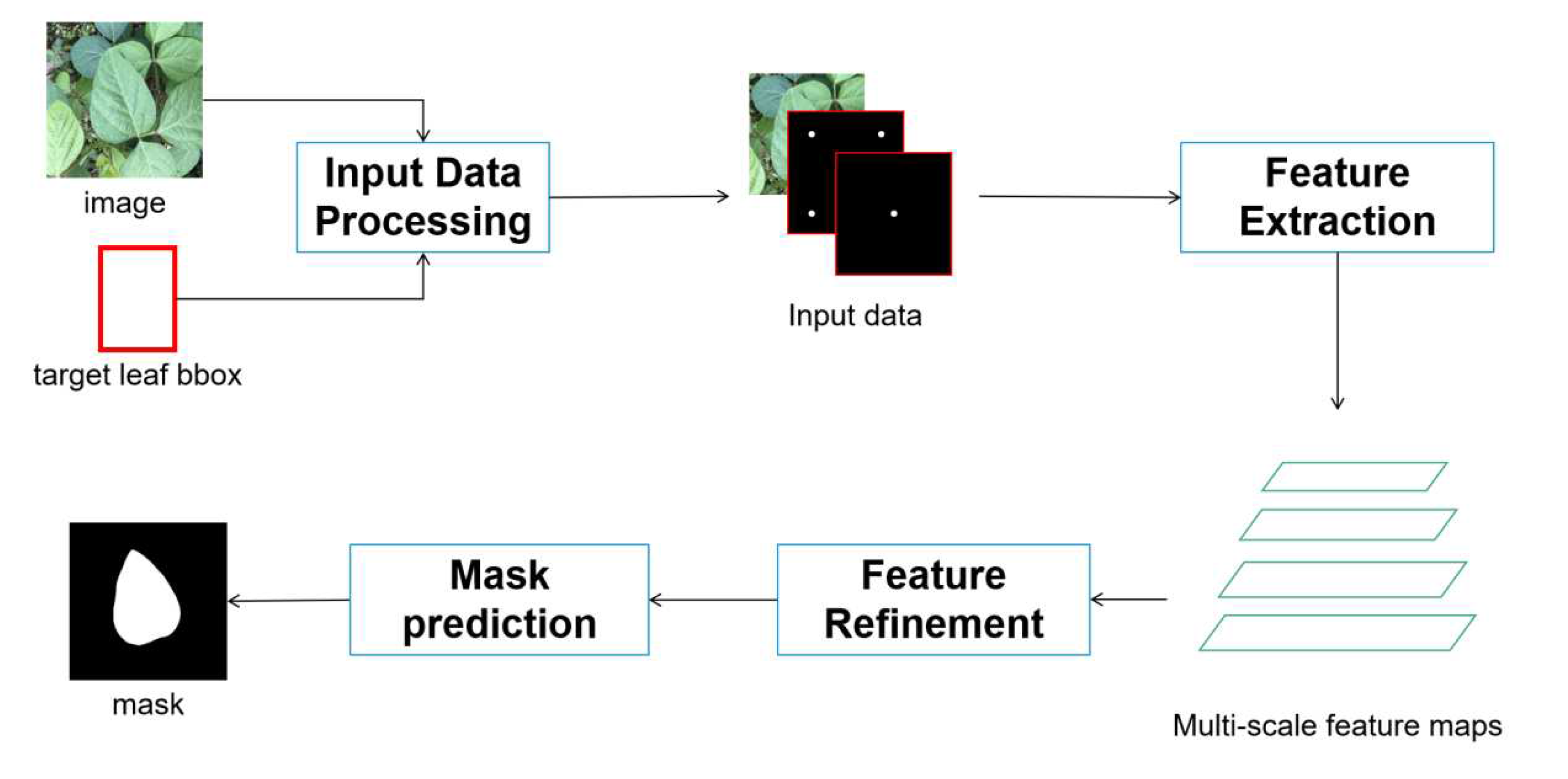
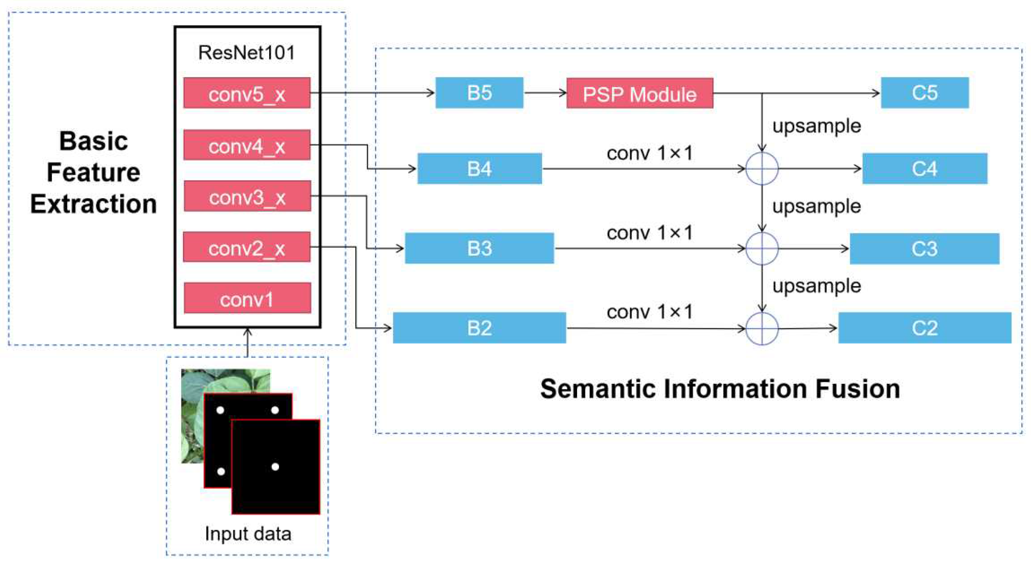
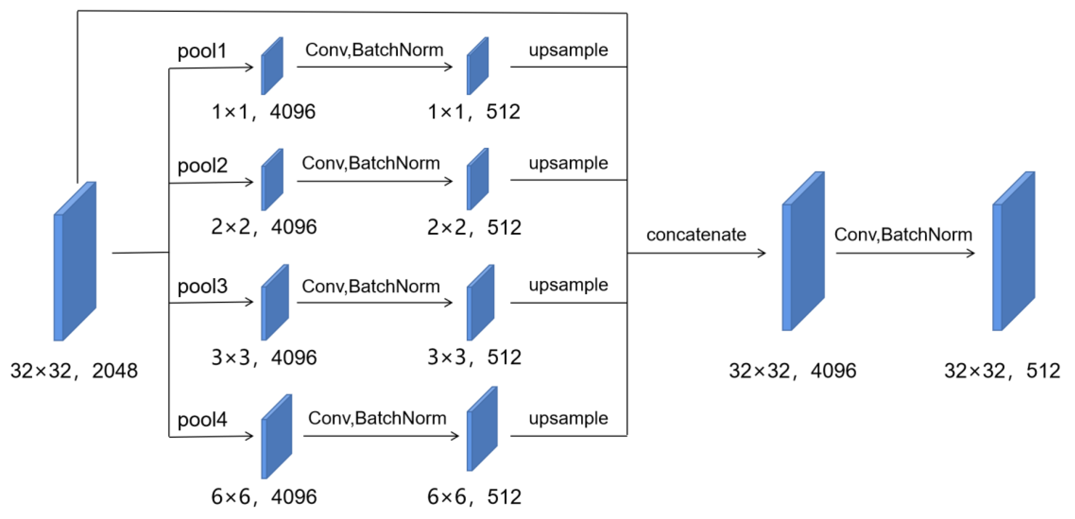
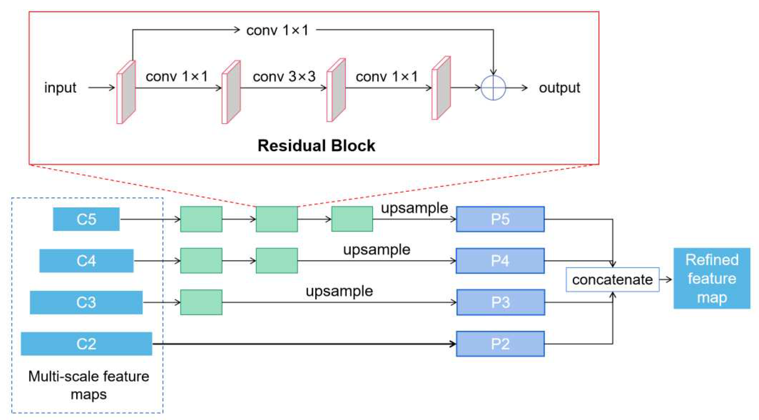
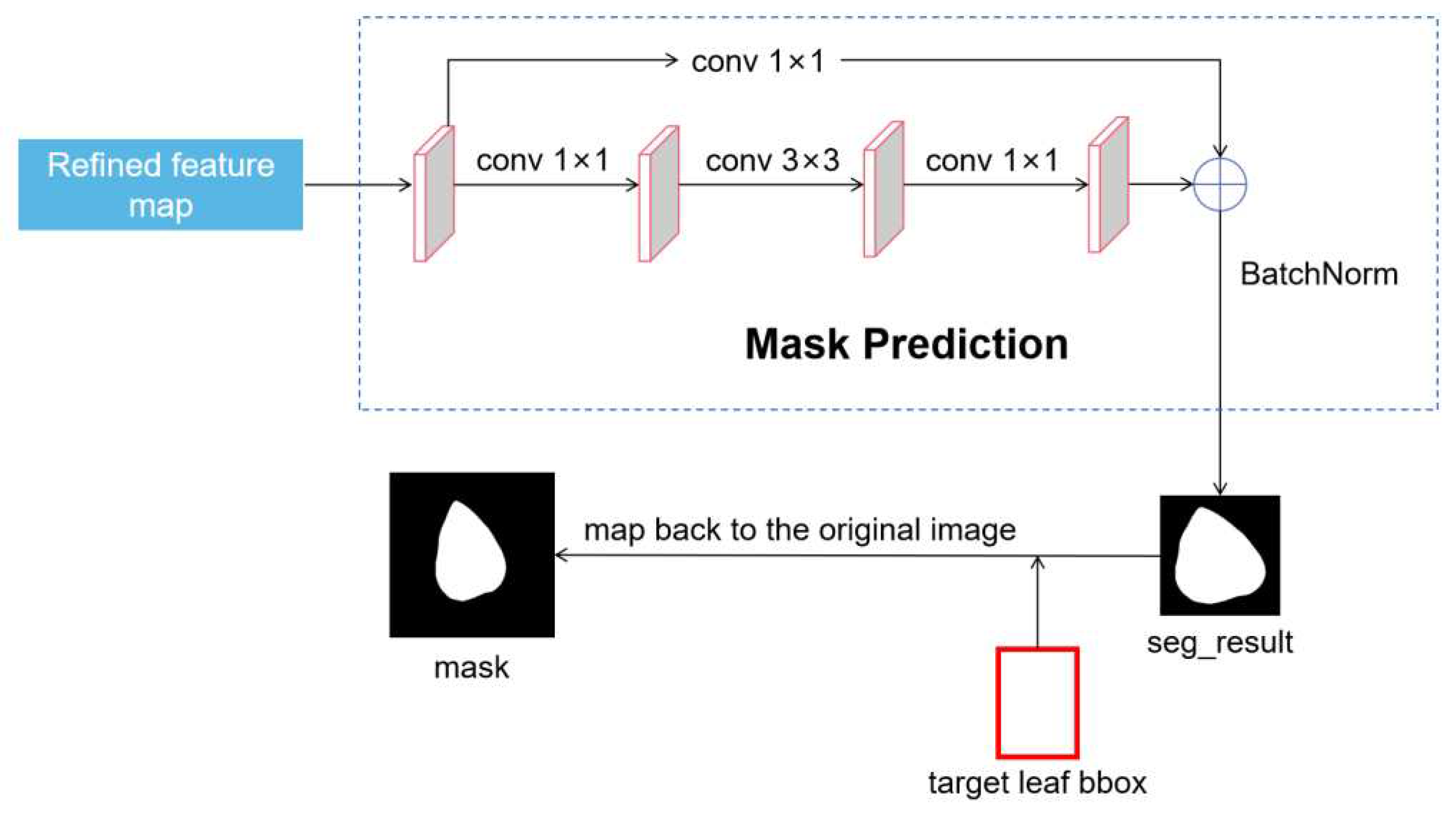
2.2.3. Target Leaf Segmentation Network

The target leaf segmentation model is consisted of four stages, as shown in Figure 11. (1) input data processing, where outside information and inside information of target leaf are given. (2) feature extraction, where the multi-scale features of the target leaf are extracted. (3) feature refinement, where the multi-scale features are upsampling and fused to repair boundary feature of segmentation region. (4) the mask prediction, where the mask of target leaf is generated.

a) Input data processing

The input data processing introduces prior guidance for target leaf segmentation model. It consists of three steps, as shown in Figure 12. (1) the part region of original image is used for target leaf segmentation. Image cropping operation is executed to obtained the part region by shifting 30 pixels outwards along the target leaf bounding box. (2) the cropped image is scaled to a standard size (e.g., 512

\times

512), and the vertex coordinates of the target leaf bounding box are adjusted accordingly. (3) two single-channel Gaussian heat maps are constructed to provide background and foreground prior guidance according to the target leaf bounding box. Using the center point coordinates (

x_{0}

y_{0}

) of the bounding box, the channel for foreground prior guidance is defined by Gaussian heat map as

F P = e^{(- \frac{(x - x_{0})^{2} + (y - y_{0})^{2}}{σ^{2}})}

(18)

where

σ = \frac{5}{\sqrt{l o g 2}}

. Similarly, using the 4 vertex coordinates {

(x_{i}, y_{i})

| i

\in

{1,2,3,4}} of the bounding box, the channel for background prior guidance is

B P = m a x {e^{(- \frac{(x - x_{i})^{2} + (y - y_{i})^{2}}{σ^{2}})} | i \in {1, 2, 3, 4}}

(18)

The two Gaussian heat maps are concatenated with the scaled image to form an input data with five channels for target leaf segmentation model.

b) Feature extraction for target leaf segmentation

The feature extraction network adopts a structure design similar to FPN, as shown in Figure 13, including basic feature extraction and semantic information fusion. In the basic feature extraction part, the ResNet101 is used to construct a pyramid structured multi-scale feature map. Unlike the general FPN structure, the deepest feature map output from ResNet101 is processed by the pyramid scene parsing (PSP) (Zhao et al., 2017) module to enrich the feature representation with global contextual information. The structure of PSP module is shown by Figure 14. Firstly, the input feature map is averaged by four pooling windows to produce four pooled feature maps with size 1*1, 2*2, 3*3 and 6*6 respectively. Secondly, these feature maps are operated in sequence by convolution, batch normalization and finally up-sampled to generate multi-scale feature maps with the same size as the original feature map. Finally, the generated multi-scale feature maps and the original feature map are concatenated and followed by convolution and batch normalization to output a feature map of semantic information fusion. After enriching the feature representation of the last layer, FPN is used to fuse the feature maps of adjacent stages through the top-down path and the lateral path.

C) Feature refinement

The multi-scale feature maps extracted from the feature extraction network lose feature details, which may destroy the boundary of segment region. The feature refinement network aims to repair the lost boundary feature by up sampling and fusing the multi-scale feature information. The structure of the feature refinement network is shown in Figure 15. Firstly, the residual block is used for feature enhancement. The number of residual blocks is different for different layers, where 3, 2, 1, 0 are for C5, C4, C3 and C2 separately. Next, up-sampling is performed on these enhanced feature maps so that their size is equal to the lowest level feature map P2. Finally, the feature maps P2, P3, P4 and P5 are concatenated to obtain the refined feature map.

d) Mask prediction

The process of mask prediction is shown in Figure 16. The refined feature map is first passed through the mask predictor to generate a target mask, and then the mask is mapped back to the original image. The predictor adopts a structure similar to the residual block. Three serial convolution layer operators act on and add the input feature map. The result is followed by a batch normalization operation to generate the mask of target leaf. According to the position and size of target leaf bounding box, the mask is mapped to the original image so as to segment the target leaf from the original image.

e) Loss function definition for leaf segmentation

In order to better supervise the model training, we not only construct the loss for the final generated mask, but also calculate the loss for the mask predicted from each level of CoarseNet (C2, C3, C4, C5). Therefore, the total loss of the model is the sum of the five losses

L = \sum_{k = 1}^{5} L_{k}

(19)

The loss

L_{k}

is defined using binary cross-entropy loss as

L_{k} = - \frac{1}{N} \sum_{i} [y_{i} \log (p_{i}) + (1 - y_{i}) \log ({1 - p}_{i})]

(20)

where

p_{i}

is the predicted value of pixel

i

of mask

k

and

y_{i}

(0 or 1) is the ground truth.

3. Experimental Results and Analysis

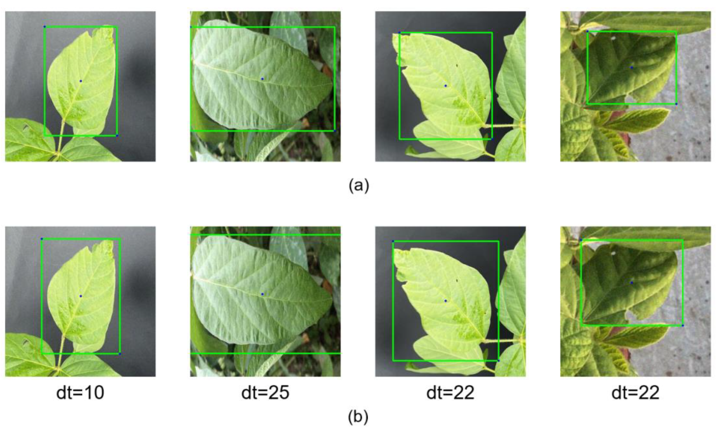
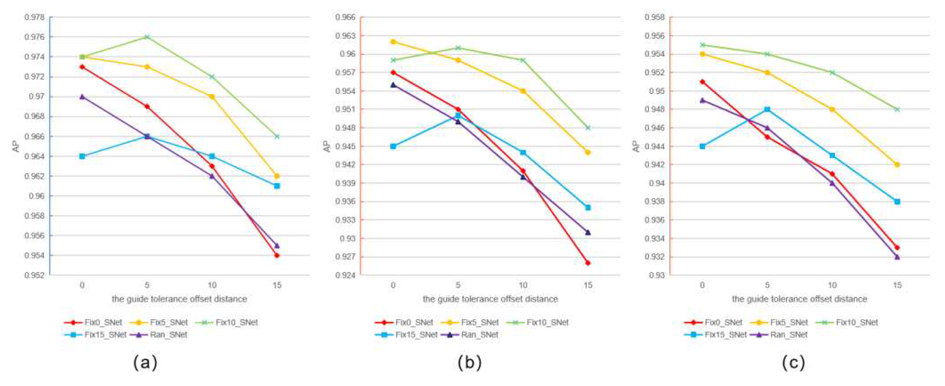
The computer configurations for the model experiments are shown in Table 1. We trained the leaf detector and the leaf segmentation network separately. The training parameter settings for the two models are shown in Table 2.

3.1. Vertex Offset Strategy for Bounding Box

The vertex coordinates of bounding box have an important impact on the leaf segmentation results. In this experiment, we explore tolerance offset distance strategy for vertex coordinates of bounding box to maximize leaf segmentation accuracy. It refers to the strategy of combining leaf segmentation networks trained by supervised data with different tolerance offset distance

d_{t}

. In this experiment, we use 0, 5, 10, 15 and random offset distance in the range of [0, 15] to train five leaf segmentation networks for comparison and analysis. These five leaf segmentation networks are called Fix0_SNet, Fix5_SNet, Fix10_SNet, Fix15_SNet and Ran_SNet. When evaluating the segmentation accuracy of the overall model, four offset distance

d_{t}

is separately tested again. So there are totally 20 combination schemes and the corresponding segmentation accuracies are shown in Figure 17a. X-axis represents offset distance

d_{t}

, Y-axis represents segmentation accuracies measured by AP and five segmentation networks are marked by five colors. We may notice the highest accuracy of 0.976 is from the combination of test

d_{t} = 5

and training

d_{t} = 10

3.2. The Affection of Leaf Detectors on the Segmentation

In order to verify the affection of leaf detector on the segmentation results, we used two popular detection models of Faster R-CNN and yolov5x in replace of Libra R-CNN. We also applied all guide offset strategies to each model and record the results of each experiment. The experimental results are shown in Figure 17(b) and (c). According to the statistics, we can see that the strategy of combining

d_{t} = 0

and Fix5_SNet can make the segmentation model achieve the highest segmentation accuracy with 96.2% accuracy by using Faster R-CNN as the detector, while the strategy of combining

d_{t} = 0

and Fix10_SNet can achieve the highest accuracy of 95.5% by yolov5x. Comparing the experimental results of the three detectors, the segmentation model using Libra R-CNN has the best segmentation performance.

3.3. Comparative Experiment

To highlight the performance of our leaf segmentation model, three baseline segmentation models, Mask R-CNN, DeepLabv3 and UNet, were compared with quantitative analysis and qualitative comparison.

3.3.1. Quantitative Analysis

The evaluation metrics of quantitative analysis adopted are Accuracy, Precision, Recall, F1 Score, AP and AR to measure the segmentation accuracy. All the models are trained and tested by our constructed soybean leaf data set, that is, 1619 images for training and 1335 images for evaluating. The statistics results are shown in Table 3. By comparing those data, we can notice that our segmentation accuracy is better than the others, which proves that our model has stronger segmentation capability.

Among those evaluation metrics, they can be divided two categories: the four metrics of Accuracy, Precision, Recall and F1 Score are used for comparison with the whole image. In segmentation task, the predicted mask pixels are compared with the ground truth, and these pixels are classified as false-positive samples, true-positive samples, false-negative samples, or true-negative samples. Due to large number of images and large proportion of background pixels in the images, the proportion of true-positive samples and true-negative samples will be too large. It induces three large indicators, which brings us the illusion of high segmentation accuracy. The evaluation values by those four metrics are closer between those models, as shown in Table 3. The other two metrics of AP and AR are used for comparison between predicted positive mask and ground truth. They divide the samples with the IoU values of the predicted mask and the true mask, and calculate Precision and Recall with IoU thresholds. The results are more persuasive. From Table 3, there are significant differences for AP and AR metrics between those models.

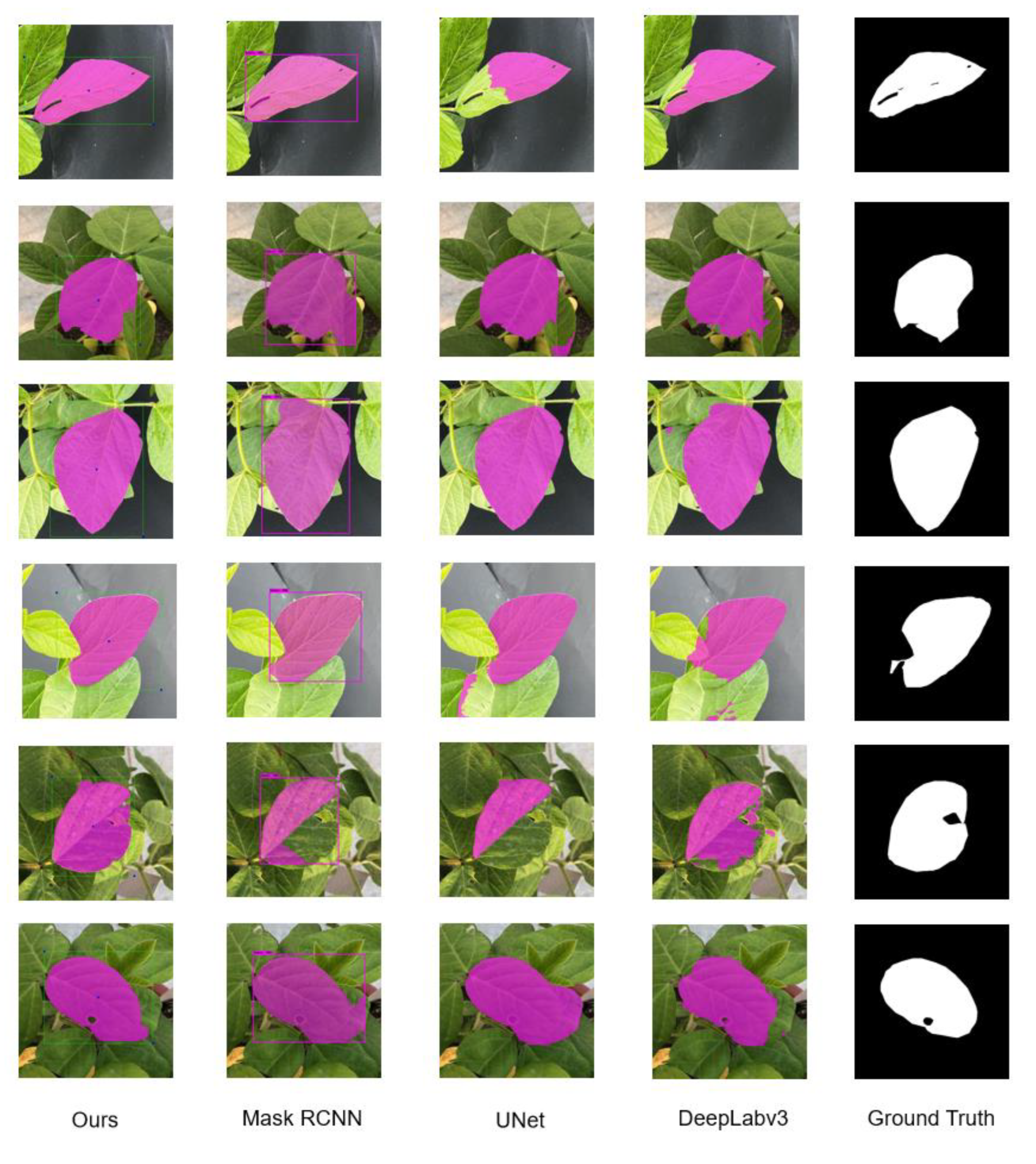
3.3.2. Quantitative Comparison

Figure 18 shows some of the segmentation results produced by the comparison methods. The data is diverse with incomplete leaves such as the second sample and occluded leaves such as the fourth sample. From the results, for the baseline segmentation models, background pixels are regarded as foregrounds, such as samples 2, 3, and 6 by mask RCNN, Samples 2, 4, and 6 by UNet, samples 2, 3, and 6 by DeepL abv3. There are also foregrounds pixels as background, such as sample 5 by mask RCNN, samples 1 and 5 by UNet, the samples 1, 4, and 5 by DeepL abv3. Although artifacts also exist in our results, such as exampls 5 and 6 where part background pixels are regarded as foreground, the segmentation effect is the best among the models. Maybe two operations play an important role. One is the high accuracy of the input bounding box for segmentation model. The other is the segmentation model is guided by inside and outside information of segmentation region.

4. Conclusions

Target soybean leaf extraction is a prerequisite for calculating the phenotypic parameters of soybean leaves. In this paper, an automatic segmentation model of soybean leaf is proposed by combining object detection and interactive image segmentation technology. Based on the idea that the target leaf is located in the center of the image and the leaf area is large, a method to locate the target soybean leaf is provided. The bounding box of target soybean leaf is optimized to achieve more accurate segmentation of target soybean leaf. Various experimental data and comparative analysis show that our model has higher segmentation accuracy and better generalization capacity.

However, because the target soybean leaf and the background soybean leaf are highly similar both in color and texture, it makes the segmentation of target soybean leaf difficult. In some cases, it is difficult to find the boundary between the target leaf and the background leaf, which may induce the wrong segmentation. As shown in Figure 19, part region of the background leaf is regarded as the foreground. In order to further improve the segmentation precision, image depth or NeRF(Neural Radiance Field) based implicit 3D reconstruction technology may be adopted to obtain more information to identify the foreground and background soybean leaves.

References

Bai, X., Li, X., Fu, Z., Lv, X., & Zhang, L. (2017). A fuzzy clustering segmentation method based on neighborhood grayscale information for defining cucumber leaf spot disease images. Computers and Electronics in Agriculture, 136, 157-165. [CrossRef]
Benenson, R., Popov, S., & Ferrari, V. (2019). Large-scale interactive object segmentation with human annotators. In Proceedings of the IEEE/CVF conference on computer vision and pattern recognition, pp. 11700-11709.
Bhagat, S. , Kokare, M., Haswani, V., Hambarde, P., & Kamble, R. (2022). Eff-UNet++: A novel architecture for plant leaf segmentation and counting. Ecological Informatics, 68, 101583. [CrossRef]
Cai, Z., & Vasconcelos, N. (2018). Cascade r-cnn: Delving into high quality object detection. In Proceedings of the IEEE conference on computer vision and pattern recognition, pp. 6154-6162.
Chandio, A. , Gui, G., Kumar, T., Ullah, I., Ranjbarzadeh, R., Roy, A. M., Shen, Y. (2022). Precise single-stage detector. arXiv preprint, arXiv:2210.04252.
Chen, L. C., Zhu, Y., Papandreou, G., Schroff, F., & Adam, H. (2018). Encoder-decoder with atrous separable convolution for semantic image segmentation. In Proceedings of the European conference on computer vision (ECCV), pp. 801-818.
Gao, L., & Lin, X. (2018). A method for accurately segmenting images of medicinal plant leaves with complex backgrounds. Computers and Electronics in Agriculture, 155, 426-445. [CrossRef]
Girshick, R. (2015). Fast r-cnn. In Proceedings of the IEEE international conference on computer vision, pp. 1440-1448.
Girshick, R., Donahue, J., Darrell, T., & Malik, J. (2014). Rich feature hierarchies for accurate object detection and semantic segmentation. In Proceedings of the IEEE conference on computer vision and pattern recognition, pp. 580-587. [CrossRef]
He, K., Zhang, X., Ren, S., & Sun, J. (2016). Deep residual learning for image recognition. In Proceedings of the IEEE conference on computer vision and pattern recognition (pp. 770-778).
He, K., Gkioxari, G., Dollár, P., & Girshick, R. (2017). Mask r-cnn. In Proceedings of the IEEE international conference on computer vision, pp. 2961-2969.
Kumar, J. P., & Domnic, S. (2019). Image based leaf segmentation and counting in rosette plants. Information processing in agriculture, 6(2), 233-246. 2). [CrossRef]
Li, Z. , Chen, Q. , & Koltun, V. (2018). Interactive image segmentation with latent diversity. In Proceedings of the IEEE Conference on Computer Vision and Pattern Recognition; pp. 577–585. [Google Scholar]
Lin, T. Y. , Dollár, P. , Girshick, R., He, K., Hariharan, B., & Belongie, S. (2017). Feature pyramid networks for object detection. In Proceedings of the IEEE conference on computer vision and pattern recognition (pp. 2117-2125). [Google Scholar]
Lin, Z. , Zhang, Z. , Chen, L. Z., Cheng, M. M., & Lu, S. P. (2020). Interactive image segmentation with first click attention. In Proceedings of the IEEE/CVF conference on computer vision and pattern recognition; pp. 13339–13348. [Google Scholar]
Liu, W. , Anguelov, D., Erhan, D., Szegedy, C., Reed, S., Fu, C. Y., & Berg, A. C. (2016). Ssd: Single shot multibox detector. In Computer Vision–ECCV 2016: 14th European Conference, Amsterdam, The Netherlands, October 11–14, 2016, Proceedings, Part I 14 (pp. 21-37). Springer International Publishing.
Liu, X. , Hu, C., & Li, P. (2020). Automatic segmentation of overlapped poplar seedling leaves combining Mask R-CNN and DBSCAN. Computers and Electronics in Agriculture, 178, 105753. [CrossRef]
Long, J. , Shelhamer, E. , & Darrell, T. (2015). Fully convolutional networks for semantic segmentation. In Proceedings of the IEEE conference on computer vision and pattern recognition; pp. 3431–3440. [Google Scholar]
Maninis, K. K. , Caelles, S. , Pont-Tuset, J., & Van Gool, L. (2018). Deep extreme cut: From extreme points to object segmentation. In Proceedings of the IEEE conference on computer vision and pattern recognition; pp. 616–625. [Google Scholar]
Pang, J. , Chen, K. , Shi, J., Feng, H., Ouyang, W., & Lin, D. (2019). Libra r-cnn: Towards balanced learning for object detection. In Proceedings of the IEEE/CVF conference on computer vision and pattern recognition; pp. 821–830. [Google Scholar]
Redmon, J. , & Farhadi, A. (2017). YOLO9000: better, faster, stronger. In Proceedings of the IEEE conference on computer vision and pattern recognition; pp. 7263–7271.
Redmon, J., Divvala, S., Girshick, R., & Farhadi, A. (2016). You only look once: Unified, real-time object detection. In Proceedings of the IEEE conference on computer vision and pattern recognition, pp. 779-788.
Ren, S. , He, K., Girshick, R., & Sun, J. (2015). Faster r-cnn: Towards real-time object detection with region proposal networks. Advances in neural information processing systems, 28.
Reynolds, M. , Chapman, S., Crespo-Herrera, L., Molero, G., Mondal, S., Pequeno, D. N., Pinto, F., Pinera-Chavez, F. J., Poland, J., Rivera-Amado, C., et al. Breeder friendly phenotyping. Plant Science, pp. 110396, 2020. [CrossRef]
Ronneberger, O. , Fischer, P., & Brox, T. (2015). U-net: Convolutional networks for biomedical image segmentation. In Medical Image Computing and Computer-Assisted Intervention–MICCAI 2015: 18th International Conference, Munich, Germany, October 5-9, 2015, Proceedings, Part III 18 (pp. 234-241). Springer International Publishing.
Rother, C. , Kolmogorov, V., & Blake, A. (2004). “ GrabCut” interactive foreground extraction using iterated graph cuts. ACM transactions on graphics (TOG), 23(3), 309-314. [CrossRef]
Song, G. , Myeong, H. , & Lee, K. M. (2018). Seednet: Automatic seed generation with deep reinforcement learning for robust interactive segmentation. In Proceedings of the IEEE conference on computer vision and pattern recognition; pp. 1760–1768. [Google Scholar] [CrossRef]
Tassis, L. M. , de Souza, J. E. T., & Krohling, R. A. (2021). A deep learning approach combining instance and semantic segmentation to identify diseases and pests of coffee leaves from in-field images. Computers and Electronics in Agriculture, 186, 106191. [CrossRef]
Tian, K. , Li, J., Zeng, J., Evans, A., & Zhang, L. (2019). Segmentation of tomato leaf images based on adaptive clustering number of K-means algorithm. Computers and Electronics in Agriculture, 165, 104962. [CrossRef]
Tian, Y. , Yang, G., Wang, Z., Li, E., & Liang, Z. (2020). Instance segmentation of apple flowers using the improved mask R–CNN model. Biosystems engineering, 193, 264-278. [CrossRef]
Wang, C. , Du, P., Wu, H., Li, J., Zhao, C., & Zhu, H. (2021). A cucumber leaf disease severity classification method based on the fusion of DeepLabV3+ and U-Net. Computers and Electronics in Agriculture, 189, 106373. [CrossRef]
Wang, P., Zhang, Y., Jiang, B., & Hou, J. (2020). An maize leaf segmentation algorithm based on image repairing technology. Computers and electronics in agriculture, 172, 105349. [CrossRef]
Wang, X. , Girshick, R. , Gupta, A., & He, K. (2018). Non-local neural networks. In Proceedings of the IEEE conference on computer vision and pattern recognition; pp. 7794–7803. [Google Scholar]
Ward, B. , Brien, C., Oakey, H., Pearson, A., Negrão, S., Schilling, R. K.,... & van den Hengel, A. (2019). High-throughput 3D modelling to dissect the genetic control of leaf elongation in barley (Hordeum vulgare). The Plant Journal, 98(3), 555-570. [CrossRef]
Xie, X. , Cheng, G. , Wang, J., Yao, X., & Han, J. (2021). Oriented R-CNN for object detection. In Proceedings of the IEEE/CVF international conference on computer vision; pp. 3520–3529. [Google Scholar]
Xu, N. , Price, B., Cohen, S., Yang, J., & Huang, T. (2017). Deep grabcut for object selection. arXiv preprint, arXiv:1707.00243. [CrossRef]
Xu, N. , Price, B. , Cohen, S., Yang, J., & Huang, T. S. (2016). Deep interactive object selection. In Proceedings of the IEEE conference on computer vision and pattern recognition; pp. 373–381. [Google Scholar]
Yang, W. , Feng, H., Zhang, X., Zhang, J., Doonan, J. H., Batchelor, W. D.,... & Yan, J. (2020). Crop phenomics and high-throughput phenotyping: past decades, current challenges, and future perspectives. Molecular Plant, 13(2), 187-214. [CrossRef]
Zhang, S. , Liew, J. H., Wei, Y., Wei, S., & Zhao, Y. (2020). Interactive object segmentation with inside-outside guidance. In Proceedings of the IEEE/CVF conference on computer vision and pattern recognition; pp. 12234–12244. [Google Scholar]
Zhao, H. , Shi, J. , Qi, X., Wang, X., & Jia, J. (2017). Pyramid scene parsing network. In Proceedings of the IEEE conference on computer vision and pattern recognition; pp. 2881–2890. [Google Scholar]

Figure 2. Image annotation samples. (a) detection samples. (b) Segmentation samples.

Figure 3. Overview of the leaf segmentation model.

Figure 4. The overall architecture of Libra R-CNN.

Figure 5. Feature extraction for leaf detection module.

Figure 6. Region proposal generation.

Figure 7. Anchor generation based on feature point of different scale feature maps. (a) three anchors from feature point in feature map P2 ; (b)three anchors from feature point in feature map P3.

Figure 8. Region proposal optimization.

Figure 9. parameter affection on target leaf localization.

Figure 10. Bounding box optimization. (a) bounding box enclosing part leaf; (b) optimized bounding box.

Figure 11. Target leaf segmentation model.

Figure 12. - Input data processing.

Figure 13. Feature extraction for target leaf segmentation.

Figure 14. PSP module.

Figure 15. Feature refinement module.

Figure 16. Mask prediction.

Figure 17. The segmentation accuracy of the model with different leaf detectors and vertex offset strategies. (a) Libra R-CNN as detector. (b) Faster R-CNN as detector. (c) Yolov5x as detector.

Figure 18. The segmentation results of different models.

Figure 19. Failure case. (a) original image; (b) segmentation result.

Table 1. Computer configuration.

Configuration	Parameter
CPU	Intel(R) Core(TM) i7 - 6700 CPU
GPU	GeForce GTX 1080 Ti
Operating system	Ubuntu 22.04 LTS
Base environment	CUDA : 11.6
Development environment	Pycharm2022

Table 2. Training setting.

Parameter	Leaf detector	Leaf segmentation network
Epoch	60	100
Learning rate	0.001	1×10^-8
Batch	4	5
Weight decay	0.0005	0.005
Momentum	0.9	0.9

Table 3. quantitative comparison.

Model	AP	AR	Accuracy	Precision	Recall	F1
Ours	0.976	0.981	0.993	0.9899	0.9901	0.99
Mask R-CNN	0.921	0.936	0.9838	0.9759	0.9778	0.9769
DeepLabv3	0.767	0.815	0.9645	0.9422	0.9584	0.9769
UNet	0.794	0.834	0.9675	0.9544	0.9521	0.9532

Disclaimer/Publisher’s Note: The statements, opinions and data contained in all publications are solely those of the individual author(s) and contributor(s) and not of MDPI and/or the editor(s). MDPI and/or the editor(s) disclaim responsibility for any injury to people or property resulting from any ideas, methods, instructions or products referred to in the content.

© 2023 by the authors. Licensee MDPI, Basel, Switzerland. This article is an open access article distributed under the terms and conditions of the Creative Commons Attribution (CC BY) license (http://creativecommons.org/licenses/by/4.0/).

Copyright: This open access article is published under a Creative Commons CC BY 4.0 license, which permit the free download, distribution, and reuse, provided that the author and preprint are cited in any reuse.

MDPI Initiatives

Important Links

Choose an area of interest and we will send you notifications of new preprints at your preferred frequency.

Disclaimer

Target soybean leaf automatic segmentation based on object detection and interactive segmentation models

Abstract

1. Introduction

2. Materials and Methods

2.1. Data Set Acquisition

2.2. Methods

2.2.1. Libra R-CNN Network for Leaf Detection

2.2.2. Target Leaf Localization

2.2.3. Target Leaf Segmentation Network

3. Experimental Results and Analysis

3.1. Vertex Offset Strategy for Bounding Box

3.2. The Affection of Leaf Detectors on the Segmentation

3.3. Comparative Experiment

3.3.1. Quantitative Analysis

3.3.2. Quantitative Comparison

4. Conclusions

References

MDPI Initiatives

Important Links

Subscribe