Preprint
Article

A Mixed Vehicle Routing Problem with Electric and Internal Combustion Vehicles and Common Carriers

Altmetrics

Downloads

178

Views

40

Comments

0

Submitted:

17 July 2023

Posted:

19 July 2023

You are already at the latest version

Alerts
Abstract
With the continuous improvement and observable benefits of electric vehicles (EVs), major logistic companies are introducing more EVs into their conventional fleets. This gives rise to a new type of vehicle routing problem with mixed vehicles, where heterogeneous internal combustion vehicles (ICVs) and electric vehicles are considered in route planning. In addition, certain deliveries that are not efficient on any type of vehicles, are outsourced to third-party common carriers. In this paper, we define this problem as a mixed vehicle routing problem with common carriers (MVRPC). The objective of such problems is to minimize the transportation costs by considering routes with ICVs and EVs, the possibility of visiting recharging stations, outsourcing options, and drivers’ layover regulations. This variant of the vehicle routing problems has many practical applications, particularly in the design of long-haul transportation and last-mile delivery services. Effective MVRPC solutions play a key role in promoting the going Green image and optimally allocating resources. The problem has received limited attention in the literature likely because addressing all the needed aspects is especially challenging. To solve the large-scale problem, we develop a branch-and-cut pricing framework that relies on strong cuts and customized labeling algorithms. Numerical experiments highlight the effectiveness of our algorithm. This success can be attributed to tailored critical resources, dynamically bounded bidirectional labeling procedures, strong dominance criteria, and implementation strategies.
Keywords: 
Subject: Engineering  -   Industrial and Manufacturing Engineering

1. Introduction

In recent years, we have witnessed a growing interest in solving environmental problems such as greenhouse gas emissions, air pollution, noise, and energy wastes in the logistic industry, especially in the transportation sector. In fact, major logistic companies and smart-city designers have launched different green energy plans, see DHL GoGreen Program (2020). Sustainability has long been a competitive factor: Consumers increasingly consider environmental aspects in their purchasing decisions. The same applies to investors who consult sustainability rankings when looking for viable investment options. In this context, the entire industry is developing ways to achieve a reduction of greenhouse gas emissions and improve their overall environmental performance in transportation optimization. Meanwhile, more and more governmental laws have been passed to regulate the emission of greenhouse gases in the transportation sector, forcing major transfers from reliance on the traditional internal combustion vehicles (ICV) to electric vehicles (EV). In addition, governments and electric car makers have intensified their coverage of required infrastructures to further boost this go-green trend, see Tesla Motors Inc. (2020).
These external factors together with mounting environmental and social awareness have triggered increasing needs for high quality solutions in this field. EV, as a serious alternative for ICV, has been utilized for city-wide deliveries and public transportation, see Asghari and Alehashem (2020). Nevertheless, EV is not as competitive as ICV from a cost perspective (Goeke et al. (2015)) and from the perspective of driving ranges. The acquisition cost of electric trucks is relatively high today even with tax remedies from local governments. All the long-range trailers in usage, e.g., BYD 8TT, are still of limited diving range within 200 miles (Semi-trailer,Wikipedia (2020)), which requires visits to rechargers en route. Other heavy-duty EVs, e.g. Rivian and Tesla Semi, are still under test production, although they claim comparable long-range capability as ICVs. To overcome the limitations, efficient management of the EV fleet for delivery planning and recharge scheduling is important for companies who are considering incorporating EVs to operate their transportation businesses. The underlying management problem is known as the vehicle routing problem (VRP), whose objective is to minimize route costs by delivering goods from a depot to a given set of customers, see, e.g, Toth and Vigo (2014).
Currently, many researchers started studying the classical VRPs for EVs, which we refer as EVRPs. To our best knowledge, all of the existing EV-related literature are focused on last-mile deliveries or short-distance routing problems without considering required constraints for long-haul transportation business, such as hours of service regulations and outsourcing options. Moreover, except for two recent heuristic works, Goeke et al. (2015); Macrina et al. (2019), no research currently addresses the size and complexity of operating a large mixed dedicated fleet.No logistic company currently relies purely on EV fleets for their business but some of them are gradually introducing EVs into their existing ICV dedicated fleet. Clearly, there is a gap between the simplistic EVRP solutions and a more comprehensive model that covers the relevant real-life constraints.
In our work, we consider the compound vehicle routing problem with mixed fleet (heterogeneous ICVs and EVs) and an outsourcing option to common carriers. We call this problem MVRPC. Compared to ICVs, energy costs for operating EVs are generally lower while the fixed costs per day of using the trucks are relatively high because of the initial acquisition costs. The driver costs for both truck types are assumed to be equal. At times, the total customer demand may exceed the capacity of the dedicated fleet. In cases where customers are located far away from the distribution center or isolated from others, it can be more cost-efficient to subcontract the shipments to a third-party carrier (common carrier) by fixed tariffs. Therefore, optimal route planning decisions for MVRPC have to find the cost trade-off among the three transportation modes. Furthermore, many governments worldwide have imposed hours of service regulations for truck drivers to avoid fatigue-related accidents, see Federal Motor Carrier Safety Administration (2011). These regulations ensure that rest periods, which called layover, are regularly taken by the truck drivers. This type of problem has many practical applications, particularly at the transportation planning stage for long-haul less-than-truckload transports and last-mile distribution services where subcontracting unprofitable shipments are standard options, see, e.g., Dang et al. (2020). Restricting real-life constraints can be considered to make the planned solutions more concrete and provide informative guidance for daily operations.
In this paper, we consider a real-world transportation planning problem MVRPC that has challenged the logistic industry for many years. In MVRPC, heterogeneous-sized ICVs and a single-sized EV are available at a single depot. The objective is to determine a set of vehicle routes, each starting and ending at the depot, so that each customer is visited exactly once. If certain shipments can be fulfilled more cheaply by a common carrier, then they are outsourced. By making the routing and outsourcing decisions optimally, the overall transportation costs are minimized. Truck capacities and EV battery capacities are observed. Delivery time windows are specified for each shipment in which the drivers must arrive the customer site within the period. Along the trips, drivers must respect the U.S. hours of service regulations to take mandatory layovers once their continuous working periods hit the time limit, which is 14 hours. The rest period is flexible within an interval long enough for all the windows to be fitted. In addition, EV recharges and power consumption are present in this problem.
Unlike in most previous publications, the vehicle usage costs depend on the length of the routes, instead of a fixed number. All the parameters and constraints discussed are deterministic. Despite its practical importance, MVRPC has received limited attention in the literature. No former work has considered the comprehensive features as we do in MVRPC.
We present here an exact algorithm for MVRPC. The algorithm is a branch-and-cut-and price (BCP) procedure based on the column generation framework. Some new features are introduced compared to the BCP algorithms in literature. The methodologies provide significant improvements in solving realistic large-scale vehicle routing problems. The contributions can be summarized as: 1) the first mixed mode optimization problem involving electric vehicles and the first work that involves multiple modes including different vehicle sizes, electric vehicles, and subcontracting option; 2) the demonstration that mixed modes are critical to profitability as well as the enabling of electric vehicles; 3) the first mixed integer linear programming arc-flow formulation for such VRP variants; 4) a new labeling algorithm that deals with layovers and recharging requirements along the route, which has a broad extension to renewable resource problems that could only be solved by meta-heuristics before; 5) three sets of cutting planes that can be introduced to other column generation framework.
The paper is organized as follows. In Section 2, we provide a short discussion of the related literature on each feature of MVRPC. We also review the existing branch-and-cut-and-price algorithms. In Section 3, we provide a problem description, parameter settings, and an arc-flow-based mixed integer linear programming formulation. Section 4 and Section 5 describe details about the proposed column generation framework, valid inequalities, and the branch-and-cut-and-price algorithm. The results of our computational experiments are presented in Section 6. Finally, Section 7 presents conclusions and opportunities for future research.

2. Literature Review

Many researchers have studied vehicle routing problems. For more comprehensive reviews, see Laporte (2007); Toth and Vigo (2014). For specific reviews on the vehicle routing problems with time windows (VRPTW), readers are referred to Kallehauge (2008). For reviews on heterogeneous vehicle routing problems, surveys are available in Toth and Vigo (2014), and an important structural study was conducted by Yaman (2006). A thorough survey provided by Pelletier et al. (2016) covers the topics and progress on electric vehicle routing problems in the past five decades. Unfortunately, there is no publication in the literature that covers the exact same features as ours. Therefore, we split the literature review into different segments. In this section, we review the specific parts of the literature that relate to our contributions. First, we review the related literature about green vehicle and mixed fleet routing, VRP with common carriers, and VRP with layover or driver’s time regulations. Second, we explore the current state of the art for the branch-and-cut-and-price algorithms in the VRP domain.

2.1. Related VRP Variants

We start by reviewing the green vehicle and mixed fleet routing problems. Conrad and Figliozzi (2011) conducted a bounding study for an EVRP with time windows and fixed recharging time. Fukasawa et al. (2016) proposed a branch-and-cut-and-price algorithm for an EVRP with time windows. In particular, Fukasawa et al. (2016) studied the strengths of different reformulations and developed the 2-cycle-free q-routes column generation framework. Schneider et al. (2014) considered an EVRP with time windows and truck capacities. Like Schneider et al. (2014), we also allow EVs to visit any available rechargers before running out of electricity. We assume that after each visit the battery is fully charged. Schneider et al. (2014) provided a non-linear mixed integer formulation and a hybrid meta-heuristic algorithm. We seek to show that a linear formulation can capture all the elements permitting greater computational efficiency.
It should be noted some authors consider richer options for recharging, while only focusing on a single type of vehicle. Desaulniers et al. (2016) studied the EVRP under four different recharging policies. The authors tailored their BCP algorithms under different scenarios and ran their models on several benchmark problems. Andelmin and Bartolini (2017) considered an alternative fuel charge vehicle with delayed recharging policy. They introduced tighter cycle elimination techniques which allow exact solutions for more than 100 customers in the previously unsolvable instances.
Although many EVRP works focus on constant or linearized electricity consumption, research that involves accurate energy estimations is of importance in providing guidance for the optimization models. For example, Arasu et al. (2019); Demir et al. (2012) both provided parameter estimation models, e.g. for powertrain recharging rates, nonlinear speed and electric consumption, and heuristic algorithms for solving energy-oriented VRPs. As mentioned before, the only two existing publications on similar mixed vehicle routing variants (Goeke et al. (2015); Macrina et al. (2019)) are focused on heuristic approaches. Apparently, none of the previous research provides a clear optimization formulation that can be solved by off-the-shelf solvers.
In terms of the VRP variants with common carriers, most of the research still relies on the field of meta-heuristics. The first work to address outsourcing options for VRPs is Chu C-W (2005). The author considered a single-depot routing problem with a less-than-truckload carrier option. The objective is to minimize the total network cost. Chu C-W (2005) solved the problem by a simple “modified savings” math-heuristic for up to 30 customers. The first work for outsourcing options with a time window is Moon et al. (2012). The authors assign deliveries to vehicles of different carriers in a greedy manner. A heuristic based on a genetic algorithm is proposed in Vidal et al. (2016). Gahm et al. (2017) introduced a new variant in which a heterogeneous dedicated fleet and multiple cost options are considered. This work involved only variable travel costs and three options on the common carrier costs. The problem is solved by a neighborhood search heuristic. More recently, Alcaraz et al. (2019) combined heterogeneous fleet types with last-mile outsourcing options and hours of service regulation (layovers). The authors employed three heuristics: simulated annealing, tabu search, and variable neighborhood search - in solving their problem. They examined the results on up to 100 shipments random instances and studied the stability of the three heuristics. Dang et al. (2020) considered the layover regulations and the outsourcing options in their work and solved the new problem by an ant colony based meta-heuristic approach. The resulting problem is called vehicle routing problem with common carriers and time regulations (VRPCCTR). A recent publication by Dabia et al. (2019,a) is the only one that focuses on exact methods. This work considered complex tariff structures for the outsourcing options. The authors provided two different set-partitioning reformulations, strengthened cuts and modified dominance criteria for the BCP algorithm. Moreover, they conducted relatively structural studies on the impacts of the outsourcing decisions to the routing decisions. Since VRP with common carriers is not thoroughly studied yet, their work yields many opportunities for further study and analysis.
The publications regarding hours-of-service regulations contain more diversified solution methodologies. Alcaraz et al. (2019) reviewed works that considered both layovers and outsourcing options. From their review, this hybrid setting is still mainly solved by meta-heuristic approaches. Goel and Irnich (2014) presented the first exact method for the VRP variants considering layover regulations. The authors proposed a branch-and-price algorithm with a forward labeling search procedure. New dominance rules involving the layover feature were introduced. Their numerical results on Solomon instances suggested the effectiveness of the algorithm. Later, Tilk (2016) improved the work of Goel and Irnich (2014) by adding cutting planes to the master problem and a bidirectional labeling search. The acceleration strategies discussed in this work are also useful in speeding up the pricing procedures.

2.2. Column Generation Algorithms for VRPs

We solve the MVRP to optimality using BCP algorithms. With BCP, an extensive formulation is linearly relaxed. The relaxation works as a master problem which is solved using column generation. Additional valid inequalities are added to strengthen the lower bounds. Integer solutions are finally reached by branch and bound, see Lübbecke and Desrosiers (2005). The column generation process iterates between the linear reoptimization of the master problem and the solution of the pricing subproblem. In general, column generation is one of the most successful large-scale exact methods in solving combinatorial optimization problems. Desrochers et al. (1992) is the first to apply column generation in the context of the VRPTW, resulting in a branch-and-pricing algorithm. Later, Kohl et al. (1999) improved the branch-and-price algorithm by introducing subtour elimination constraints and two-path inequalities which resulted in the branch-and-cut-and-price. An additional line of research focuses on valid inequalities for column generation algorithms based on the variables of the master problem. For example, Jepsen et al. (2008) proposed a set of valid inequalities called subset-row inequalities with the variables in the Dantzig-Wolfe master problem. SR inequalities have been observed to effectively improve the lower bounds. Petersen et al. (2008) discovered how to apply generalized Chavátal-Gomory cuts to speed up the column generation solutions in the context of VRPTW. More recently, Dabia et al. (2019,b) studied the strengths of robust and non-robust cover inequalities applied on BCP algorithms. Some column generation methods often show very slow convergence partly due to heavy degeneracy problems (Rousseau et al. (2007)). Such problems arise when multiple dual solutions are associated with each primal solution. Rousseau et al. (2007) showed that the interior point method helps in stabilizing the column generation algorithms for VRPTWs.
While the master problem for most VRP variants is standard, the pricing algorithms for the subproblems are differentiated. Back in the 1990’s and earlier, researchers treated subproblems as a shortest path problem with resource constraints. Exact dynamic programming and 2-cycle eliminations were developed to price the columns with negative reduced cost, see Desrochers et al. (1992). Irnich and Villeneuve (2006) improved the elimination capability from 2-cycles to k-cycles, which increases the lower bounds of the relaxation solutions. However, the procedure is NP-Hard. Nowadays researchers mostly regard the pricing subproblem as an elementary shortest path problem with resource constraints. This consensus is attributed to the contributions of Feillet et al. (2004); Righini and Salani (2006 2008). Their works are cornerstones for the so-called labeling algorithm. The authors also introduced various accelerating techniques such as bounding, state-relaxation, bidirectional labeling search, and decremental state space relaxation, etc. Tilk et al. (2017) further improved the bidirectional labeling algorithm by dynamically adjusting the midpoint so that the number of labels generated by each direction can be controlled to a low level. Another group of researchers are focused on developing heuristic pricing algorithms to speed up the solutions for subproblems. For example, Desrochers et al. (1992) proposed a tabu search heuristic to quickly price the elementary paths with negative reduced cost. By far the most widely used route relaxation method is ng-routes, which was introduced by Baldacci et al. (2011). The method was proved by many researchers to be effective in solving difficult VRPTW instances.

3. Problem Description and Formulation

The MVRPC is an updated version of the transportation mode decision problem discussed in Dang et al. (2020). This strategic planning problem is mostly valued by logistic practitioners. Currently, major transportation companies are quantitatively evaluating the benefits of introducing electric vehicles into their fleets. They are interested in how EVs can change their current mode decisions between the dedicated fleet and common carriers. They also want to know how many more resources (e.g., rechargers, labors,etc.) should be put in order to accomplish the transitions. In this section, we describe the problem in detail and provide a formal mathematical model.

3.1. Problem Settings

We state the assumptions and policies that support the modeling of MVRPC. All dedicated fleet routes (ICVs and EVs) must start and end at the same depot. The average speed of every truck type is assumed to be constant and the same. While we regard the ICV fleet as containing multiple truck types differentiated by heterogeneous sizes, we assume there is only one type of EVs because they are single-sized. The demands for each shipment are inseparable, which means they can either be consolidated on a route or be entirely outsourced to a common carrier. Each shipment that is not outsourced must be visited exactly once by exactly one route traveled by one type of truck. A vehicle must visit the nodes within its corresponding time window such that no waiting time or late delivery is permitted. Furthermore, we assume the time windows for the rechargers and the depot are relaxed, which means they can be visited anytime that they are needed. This setting gives decision makers the data needed to optimally schedule the limited rechargers. Whenever a recharger is visited, the battery is fully recharged and the time will be counted. Yet, such time will not be regarded as working time subjected to the hours of service regulation. To make our problem more general, we do not consider the subtle break period as regulated in Federal Motor Carrier Safety Administration (2011). Instead, we only request that drivers take a layover period between 10 and 14 hours once their uninterrupted working time reaches the 14-hour limit. We realize that some previous literature considered curb weight, road infrastructures, traffic conditions in computing power consumption on a given trip, Arasu et al. (2019); Goeke et al. (2015). In our work, however, we assume that the EV fleet has a constant unit electric consumption per mile. Then the consumption on the arc is linear to the distance.

3.2. Mixed Integer Linear Formulation

The MVRPC is defined on a directed complete graph G ( I ¯ 0 , A ) , where I ¯ 0 = { 0 , 1 , . . . , n , e 1 , . . . , e m } denotes the set of nodes and A = { ( i , j ) I ¯ 0 × I ¯ 0 : i j } is the set of arcs. Node 0 represents the depot at which all the vehicle routes start and end. The nodes in I = { 1 , . . . , n } represent the customers, while E = { e 1 , . . . , e m } is the set of recharging stations. The recharging stations may share the same locations because it is extremely expensive to establish and operate high-voltage rechargers in separate locations. The combination of customers and recharging stations are denoted as I ¯ . Inclusion of the depot is indicated by subscripting the respective set, e.g., I 0 , I ¯ 0 , E 0 . Each node i I ¯ is associated with a demand ω i , a time window [ a i , b i ] , and a service time λ i . Note that the demand and the service time are positive for i I and 0 for i E . Each arc ( i , j ) A is associated with a non-negative travel distance d i j , and an estimated energy consumption δ i j determined by models discussed in Arasu et al. (2019). We assume constant energy consumption in analyzing applications in the logistic industry in which vehicles usually carry full truckloads. When payload distribution is considered, the energy assumption term δ i j becomes a function of total vehicle weight en arc. Due to operational requirements, a maximum-allowed intra-node distance d m a x is enforced to rule out infeasible arcs. A mixed dedicated fleet consisting of electric vehicles (EVs) and internal combustion vehicles (ICVs) is available at the depot, where ICVs are usually diesel-powered trucks. Let V = V D { e } be the set of truck types, where V D denotes the set of heterogeneous diesel trucks and { e } is the available homogeneous electric trucks. Each truck of type k V has a limited capacity Q k , a fixed cost f k , a stop cost p for each delivery, and a finite number of trucks n k available. For all fleet types k V , we use the same averaged speed g = 55   m ph . Furthermore, for all arcs ( i , j ) A and fleet types k V , let c i j k be the travel cost from node i to node j, where c i j k is an average of drivers’ wages and fuel cost for ICVs and an average of driver’s wages and energy cost for electric trucks. Since there is no reason to operate an ICV route from customer sites to recharging stations, or vice versa, we define an infeasible set that represent these arcs. Let A represent the infeasible arc set, where A = { ( i , j , k ) , ( j , i , k ) : i I ¯ 0 , j E , k V D } .
On each visit to a recharger, electric trucks are recharged to their maximum battery capacity φ . The recharging time depends on the recharging rate α and the remaining electrics on arrival at the recharger. Common carriers are available for which demand can be outsourced. If customer i I is outsourced to a common carrier, the corresponding cost is retrieved from the tariff as m i . According to U.S. governmental hours of service regulations, the truck drivers need to take a layover when their working time reaches the upper threshold ξ = 14 hours, where the layover period is specified between β l b = 10 hours and β u b = 14 hours (according to industry conventions).
Thereafter, MVRPC can be formulated as a mixed integer linear program (MILP). For every arc ( i , j ) A and k V , let x i j k be a binary variable that takes value 1 only if fleet type k travels arc ( i , j ) and 0 otherwise with x i j k = 0 is fixed if ( i , j , k ) A . Let y i be a binary variable which takes the value 1 only if customer i is subcontracted to a common carrier and 0 otherwise. Continuous variables s i k define the arrival time at node i by truck type k and u i is the accumulated demands from the depot up to node i. Continuous variables z i trace the remaining battery level on arrival at node i. t i is defined as the remaining working time before a layover on arrival at node i. r i k is used to determine the hours taken by the driver for layovers immediately before node i and l i k is the number of layovers needed precedent i. To keep the notations consistent in the formulation, we define l 0 k = { l 10 k , l 20 k , . . . , l e m 0 k } as a ( n + m ) × 1 vector for each k V , where l i 0 k represents the number of layovers needed on the way back to depot. Note that r i k = l i k = 0 for all k V D and i E .
For clarity, we summarize the parameters and variables of the MILP model in Table 1.
This problem ( P ) can be represented by the following arc flow formulation:
min a a k V { f k ( i I ¯ 0 l i k + i I ¯ x i 0 k ) + ( i , j ) A [ ( c i j k + p ) x i j k ] i I ¯ p · x i 0 k } + i I m i · y i
s . t . k V D j I 0 x i j k + j I ¯ 0 x i j e + y i = 1 , i I , i j
i I x 0 i k n k , k V D
i I ¯ x 0 i e n e
j I ¯ 0 x i j e 1 , i E , i j
i I 0 , i j x i j k = h I 0 h j x j h k , k V D , j I
i I ¯ 0 , i j x i j e = h I ¯ 0 h j x j h e , j I ¯
b i s i k a i i I ¯ , k V s j e s i e + ( d i j g + λ i ) + r j e + α · ( φ z i ) ( 1 x i j e ) · M ,
i E , j I ¯ 0 , i j s j k s i k + ( d i j g + λ i ) · x i j k + r j k ( 1 x i j k ) · M ,
k V , i I 0 , j I ¯ 0 , i j
z i δ i j · x i j e + φ · ( 1 x i j e ) z j , i I , j I ¯ 0
φ δ i j · x i j e z j , i E 0 , j I ¯ 0 , i j
ξ · l j k + t i ( d i j g + λ i ) · x i j k + ξ · ( 1 x i j k ) t j , k V , i I ¯ , j I ¯ 0
ξ · ( l j k + 1 ) d 0 j g · x 0 j k t j , k V , j I ¯
β u b · l i k r i k β l b · l i k , k V , i I ¯ 0
u i u j + k V Q k · x i j k ω i · y i ω j + k V j I ¯ 0 x i j k · Q k , i , j I ¯
k V Q k j I ¯ 0 x i j k + ω i · y i u i ω i , i I ¯
d i j · x i j k d m a x , ( i , j ) A , i 0 , j 0 , k V
x i j k , y i { 0 , 1 } ( where x i j k = 0 , ( i , j , k ) A ) ( i , j ) A , i I ¯ , k V
l j k Z * ; t j , z j , u i , r j k , s j k R * , k V , i I ¯ , j I ¯ 0 .
The objective function (1) minimizes the total fixed costs, travel costs, and outsourcing costs. Constraint (2) ensures that a customer node that is not outsourced is visited exactly once by a type-k truck. Constraints (3) and (4) ensures that the number of trucks in use is less than the available trucks for each type k. Constraint (5) guarantee that if a recharger i is visited, it can be used at most once. Constraints (6) and (7) are the flow conservation constraint of the trucks. Constraints (8)-(10) guarantee the customer time windows are respected, with variable layovers and recharging time added if necessary. It is important to set M and M as small as possible so that constraints (9) and (10) are tight enough but still valid. Here, we let M = d i j g + λ i + α · φ + T · β u b + b i , where T is a constant parameter that equals 1 for all i , j 0 and equals an integer that refers to the largest possible layover numbers between depot and any node. Furthermore, we let M = T · β u b + b i . Constraints (11) and (12) specify the electric consumption on each arc, which follow the non-decreasing rule. Constraints (13) and (14) trace the moves of truck type k along each arc to add necessary layovers. Again, the layover period and work time follow the non-decreasing rule node by node. Next, constraint (15) ensures the dynamic layover time added to truck type k obeys the hours of service regulation. The subtour elimination constraints (16), (17) are extended from Dang et al. (2020) to the heterogeneous case. Constraint (18) ensures the intra-node distances are feasible. Finally, we define the domains for each decision variable in constraints (19) and (20).

4. The Set Partitioning Formulation

The set partitioning (SP) formulation has been successfully applied to solve large scale CVRP instances and crew scheduling problems because of its tight linear programming (LP) which motivates our choice of an SP reformulation for MVRPC.In addition to the parameters and variables shown in Table 1, the following additional notations are needed. We define Ω k as the set of feasible dedicated fleet routes that can be fulfilled by vehicle type k V . A dedicated fleet route is feasible for vehicle type k if and only if the delivery windows, capacity constraints, layover requirements, and the intra-node distance are all satisfied. Then, we define Ω = k V Ω k = k V D Ω k Ω e to be the set of all columns (feasible routes). For each route q Ω , let c q denote the cost, which includes the fixed cost and the variable travel cost. Let η i j q be the number of times arc ( i , j ) is visited by route q and x q be a binary decision variable that takes value 1 if and only if route q is included in the current solution. Again, η i j q = 0 such that ( i , j , q ) A . The MVRPC is formulated as the following SP problem ( R ) :
min a a q Ω c q · x q + i I m i · y i
s . t . q Ω k : k V D j I 0 η i j q · x q + q Ω e j I ¯ 0 η i j e · x q + y i = 1 , i I
q Ω k x q n k , k V
x q { 0 , 1 } , y i 0 , q Ω , i I .
The objective function (21) minimizes the cost of the selected dedicated fleet routes (columns) and the cost charged for outsourcing shipments to the common carriers. Constraint (22) is the degree constraint that is projected to the space of ( i , j , q ) , which ensures that each shipment is either served by a type-k truck or is outsourced to a common carrier. Constraint (23) guarantees that the number of occupied trucks does not exceed the available number n k of each fleet type. Next, constraint (24) sets the domain of decision variables.

4.1. Cutting Planes on Restricted Master Problem

To further tighten the LP bounds obtained from the SP formulation, we can add additional constraints satisfied by all feasible solutions into ( R ) . One way to obtain additional constraints in the ( x q , y i )-space is through the transformation of valid inequalities in the space of other variables. For examples, some well-known valid inequalities in the ( x i j k )-space derived for HVRP are also valid for MVRPC. The reason is that their three-index flow formulations share the same feasible set. However, those valid inequalities are no longer strong because of the existence of y i . When the ( x i j k )-variables and the ( x q )-variables both refer to the same feasible route, the coupling constraints between them can be defined as in constraints (25). Then, any valid inequality in the ( x i j k )-space can be lifted and transformed to a valid inequality in the ( x q , y i )-space.
x i j k q Ω k η i j q · x q = 0 , ( i , j , k ) A
Constraints (23) are the obvious projection of constraints (3) and (4) from the ( x i j k )-space to the ( x q )-space. Considering that constraints (3) and (4) hold and i I x i 0 k = q Ω k x q i I η i 0 q = q Ω k x q holds, we thus have q Ω k x q n k , which is exactly constraints 23.

4.1.1. Chvátal-Gomory Rank-1 Cut

Leveraging this fact and constraints (25), we first study the Chvátal-Gomory (CG) rank-1 cuts that can be applied to ( R ) and strengthen the LP relaxation.
Consider a general IP and its polyhedron.
min { c x : A x b , x 0 , x Z n }
P I P = c o n v { x Z n : A x b , x 0 } = c o n v ( P L P Z n )
A Chavátal-Gomory (CG) cut is a valid inequality for P I P :
u A x u b
where A is a m × n integral matrix and b Z m . The continuous parameter u R + m arises from the valid CG cuts (Conforti et al. (2014). Note that CG cuts depend on P L P and not directly on P I P , i.e., a different LP formulation of the same IP problem can produce different CG cuts (Fischetti et al. (2007)). Inequality (28) is said to have rank-1 with respect to the polyhedron P L P . Then the separation optimization problem is defined as follows. Given a point x * P L P , the CG separation problem consists of finding a CG cut that is violated by x * , i.e., finding u 0 such that u A x * > u b , or proving that no such u exist. Given the fractional input x * to be separated, the maximally violated CG cut for some non-negative u can be found by solving the following MIP (Conforti et al. (2014)):
max a a u A x u b
s . t . u A j u A j , j N
u b > u b 1
u i 0 , i M
u A j , u b Z , j N .
It was shown by Gomory that every fractional vertex x * of P L P associated with a certain basis B of ( A , I ) can be cut off by the CG cut in which u is chosen as the i t h row of B 1 , see Gomory (1958). Moreover, since only basis variables with non-zero values can contribute to the violation of the CG rank-1 cut, all zero-valued variables can be left out of the formulation which is how CG cuts are added to the simplex algorithm. As for MVRPC, the CG rank-1 cuts are based on constraints (22). With u 0 , the CG rank-1 cut with respect to the restricted master problem (RMP) (21) and (22) is given as:
q Ω k : k V D i I u i j I 0 η i j q x q + q Ω e i I u i j I ¯ 0 η i j q x q + i I u i y i i I u i
Proposition 4.1. 
CG rank-1 cuts (34) are valid for the SP problem ( R ) .
Proof. The proof follows the definition of CG rank-1 cuts, see Chvátal (1973). Consider constraints (22) with a vector u 0 , then we have u A x i I u i u A x i I u i . This step actually weakens the inequality. To avoid badness, we can designate u, s.t. u A is an integer, so u A = u A . Also, since x q , y i { 0 , 1 } , we have u A x i I u i , where A stands for the matrix formed by η i j q ’s and 1’s. This is a standard format of inequality (34). □
Therefore, given a fractional solution x from the RMP, the separation problem of finding the most violated CG rank-1 cut is again the MIP problem (29). Without loss of generality, we can choose the u i s equal to ω i , so that the weight of each node is captured in (34). Since the CG cut (34) is valid for the entire customer set I, it should also hold for S I . However, the opposite direction does not necessarily hold, as we will see in Example 1. This results is a so-called sub-row (SR) inequality, see Jepsen et al. (2008). Since SR inequality has been successfully implemented to related BCP algorithms by many previous researchers, e.g., Jepsen et al. (2008) and Dabia et al. (2019,a), we can also extend the inequality to MVRPC as a special case of CG rank-1 cuts.
q Ω 1 ϕ i S ω i σ i q x q + i S ω i ϕ y i i S ω i ϕ
where S I and 0 < ϕ ω ( S ) . σ i q is a constant that counts the number of times node i is visited by route q. This is equivalent to the set of CG cuts (34), where | S | of the ω i ’s are divided by ϕ and the rest are set to 0, i.e., u is designed as a very sparse vector.
Example 1. 
Let’s consider a simple numerical example with u i ’s as in constraint (35). The route decision variables x q ’s and the subcontracting decision variables y i ’s are all fractional. Let u i = ω i ϕ , where 0 < ϕ | I | 1 . Let k V . Assume in the current iteration, we have 3 columns generated ( q = 3 ) and 5 shipments in. Table 2 reports the fractional solutions and associated parameters obtained by solving the RMP. Let’s consider a CG rank-1 cut of the form (34) and a SR cut of the form (35) with S = { 2 , 3 } and ϕ = 5 . By substituting the variables and parameters with the real values, we have the CG cut:
2 x R 1 + 2 x R 2 + x R 3 + y 1 + y 5 3
While the corresponding SR inequality is:
x R 1 + x R 2 1
With the fractional values added, we have the CG cut be 3.1 3 , but the SR inequality be 0.7 1 . Therefore, the derived CG cut is violated whereas the SR inequality is not. However, if we choose s = { 1 , 5 } , then the SR cut is x R 1 + x R 2 + x R 3 + y 1 + y 5 2 , which indicates 2.4 2 . The SR cut is more violated than the general CG rank-1 cut. This example indicates that SR cut is not always robust and the separation optimization are important to identify efficient CG rank-1 cuts at each branching node. In fact, Fischetti et al. (2007) suggested strong cuts correspond to “minimal” CG multiplier vectors with as few nonzero entries as possible because of the cumbersome separation time and the cut strength. In addition, the experimental results in Petersen et al. (2008) showed that there is barely no difference between the LP bounds of CG rank-1 and SR cuts on VRPTW instances. Therefore, to speed up the cut generations, we use SR inequalities in the BCP algorithms.
Table 2. Fractional decisions for the outsourcing options (left panel) and the dedicated fleet routes (right panel).
Preprints 79742 i006
As in Jepsen et al. (2008); Petersen et al. (2008), we consider a subset S I with three shipments. The subset row inequalities are separated by enumerating all subsets of three shipments and checking for each subset whether the corresponding inequality is violated. Violated inequalities are added to the RMP. And the separation problem of SR inequalities is defined as follows: given the current LP solution x where x q < 1 for all q Ω , find the most violated inequality (35), such that:
max q Ω 1 ϕ i S ω i σ i q x q + i S ω i ϕ y i i S ω i ϕ
Jepsen et al. (2008) has proved that optimizing the problem (38) is NP-Complete. Therefore, we introduce simple separation heuristic ideas to identify the subset S that leads to the most violated SR inequality in each column generation iteration. Firstly, we check any three shipment combinations from every priced column (route). Then, we add the top three violated SR inequalities to the RMP. Meanwhile, we store the ten nearest shipments in an adjacent list for each shipment i I , so that each possible subset of three is checked for violation of the SR inequality. In this way, the algorithm will not be slowed down by optimizing the separation problem in a single iteration.

4.1.2. 2-path Inequalities

2-path inequalities were introduced by Kohl et al. (1999) for VRPTW and have been widely applied in multiple BCP algorithms in solving different variants of VRPs, e.g., Desaulniers et al. (2016). Similar to Desaulniers et al. (2016), we define S I to be a subset of vertices in I ¯ 0 that includes at least one shipment, and assume it is not possible to serve all shipments in S with a single truck. Here, we only consider the shipments to simplify the problem because we assume that no feasible ICV route will pass through a recharger. The corresponding 2-path inequality is given by:
q Ω ( i , j ) ( I S , S ) η i j q · x q 2
Following the separation heuristic proposed by Kohl et al. (1999), we generate the candidate sets S with the cardinality | S | 6 that satisfies q Ω ( i , j ) ( I S , S ) η i j q · x q < 2 . In other words, we generate S such that the flow entering S is the current solution of the RMP. Next, each subset S is tested to determine whether or not more than one truck is needed. If i S ω i > Q m a x , then a violated inequality (39) is identified, where Q m a x is the capacity of the maximal fleet size. If none of the violations can be found, we replace Ω with Ω k and Q m a x with Q k ( k V ) to incorporate the checks for each fleet type. In addition, if the capacity fits, we solve an elementary shortest path problem with time windows over S { 0 , 0 } , where 0 is introduced here as a duplicate of the depot that represents the destination of the route. The reduced cost of each arc ( i , j ) is set as -1 and the truck capacity is Q m a x . When the solution cost is less than | W | = 6 , it indicates this subset of shipments can be served by a single truck. Since solving this shortest path problem is extremely time-consuming, we only apply the solution procedure for the largest truck to identify violated inequalities (39).

4.1.3. Generalized Large Multistar Inequalities

Multistar inequalities are exponential VIs for Capacitated VRP problems and have been successfully implemented in different branch-and-cut and branch-and-cut-and-price algorithms, see Fukasawa et al. (2006 2016); Letchford et al. (2002); Yaman (2006). This type of VIs cut the graph G { 0 } into two sets, i.e., selected subset S I ¯ and its complementary set I ¯ S . So, instead of considering the flow into a single node, these VIs imply that the remaining capacity on the trucks entering S should be at least the demand flow of S and the flows that satisfy the demand in the node sets outside S. Multistar inequalities can be adapted to the RMP by considering the set partitioning variables and introducing the demand outsourcing variables y i . Therefore, we have:
q Ω ( i , j ) ( I ¯ S , S ) ( Q q ω i ) · η i j q x q ω ( S ) i I ω i · y i + q Ω ( i , j ) ( S , I ¯ S ) ω j · η i j q x q
To separate these inequalities, we follow the heuristic that is similar to a separation procedure for 2-path inequalities (Kohl et al. (1999)). We first enumerate all subsets S I ¯ such that | S | is less than or equal to nine, where the flow entering S is less than two, and constraints (22) are satisfied for all i S . If the inequality (40) is violated, then we store it and repeat the procedure until we reach a specified number of iterations set to 200. If not, we check whether the energy consumption on path S { 0 , 0 } is more than the battery capacity times the possible rechargers on the path plus one. If the consumption exceeds the threshold, then this flow is not feasible for an EV.
Note that both the 2-path inequalities and the generalized multistar inequalities are robust, therefore incorporating them requires no adjustment in the structure of the pricing problem. The violated 2-path inequalities and generalized multistar inequalities are added to the RMP. The shadow prices associated with the two types of cuts for subset S must be subtracted from the reduced cost of all arcs ( i , j ) ( I S , S ) .
As researched by Jepsen et al. (2008), CG rank-1 cuts (SR inequalities) are nonrobust inequalities, meaning that adding them to the RMP destroys the structure of the pricing problems. The reason is that the indicator parameters η i j q are summed over the rows and the reduced cost of the violated path can only be observed when the path is generated. Thus, the dual variables cannot be subtracted directly by the related arc ( i , j ) A . Details of how to implement the cuts in the pricing problem will be discussed in Section 5.

5. Column Generation and Pricing Problems

Given a primal LP optimal solution for the restricted RMP, the pricing problem tries to find a dedicated fleet route (a column) with a negative reduced cost if there exists one. We use the column generation framework (Lübbecke and Desrosiers (2005)) to solve the LP relaxation of (21)-(24), i.e., we consider a restricted master problem containing a subset of the columns p and generate additional columns as needed. Starting with a state where all shipments are outsourced ( y i = 1 , i I ) ), we generate additional columns for the master problem. This framework requires solving k similar subproblems for each fleet type, while the remaining unrouted shipments are handled by the y i ’s in the master problem.

5.1. Dedicated Fleet Pricing Problem

In this section, we describe the pricing problem in detail. Let μ i R ( μ i 0 ) for i I be the dual variables associated with constraints (22) and γ k R ( γ k 0 ), k V be the dual variables associated with constraints (23). Let c ¯ q , q Ω be the reduced cost of a complete path q that is operated by a type k truck, i.e., a closed loop route that starts and ends at the depot. The pricing problem without strengthened cuts for the problem ( R ) can be formulated as follows.
min q Ω k : k V D c ¯ q = c A T x = c q ( i , j ) A η i j q · μ i + γ k
We first write down the calculation of c q in (41) explicitly, c q = f k + f k · l q + ( i , j ) A ( c i j k + 1 2 p ) · η i j q . Here, we use l q to denote the number of layovers spent on path q. A feasible route in Ω is an elementary path starting and ending at the depot in which every node is visited exactly once, i.e., no loops or subtours exists. However, not all elementary paths are feasible as they may violate the time windows, truck capacities, battery capacity, or the intra-node distance constraints. The recharging time and layover time should be applied on the elementary paths if necessary to check if time windows of the shipments are respected. These resource constraints are required to be defined and traced while extending the paths. The functions that record the constraint-related resources are called resource extension functions (REFs , see Desaulniers et al. (1998)).
Problem (41) aims at finding a feasible dedicated fleet route with vehicle type k with the minimum reduced cost. The arc cost c i j k for ( i , j , k ) A A is replaced by a defined edge cost c ¯ i j k = c i j k + 1 2 p μ i , where μ 0 = μ 0 = 0 . In order to include the three types of cuts, the reduced cost of the pricing problem needs to be adjusted accordingly. Firstly, let π be the dual value associated with the 2-path cuts (39) and τ be the dual value associated with the generalized multistar cuts (40). Then, for a given shipment candidate set S, π and τ are subtracted from the reduced cost c ¯ i j k of all arcs ( i , j ) ( I S , S ) , such that ( i , j , k ) A . Therefore, we have the modified reduced cost for columns of type-k vehicle in the RMP as follows.
c ^ q = c ¯ q ( i , j ) ( I S , S ) η i j q · τ ( i , j ) ( I S , S ) η i j q · π
Similarly, consider a violated SR inequality of the form (35), defined by a subset of three shipments S r I , ϕ | S r | , and χ r < 0 as its associated dual value. Since χ is negative, it will act as a penalty. Because the terms of SR inequalities are summed over the “rows", the penalties cannot be added directly to each arc. The value χ must be subtracted from the reduced cost c ^ q each time a new column q is passed to the master problem but the column revisits shipments in S r that define the violated SR cuts. Therefore, an additional resource is required for each violated SR cut to indicate the regeneration times of the shipments. Note that we know such a column is regenerated only if completed, because the total demands fulfilled and other shipments on route could possibly change the left-hand side of the cuts. We have the updated reduced cost for the type-k column as below.
c ˜ q = c ^ q 1 ϕ i S ω i σ i q · χ r
In this setting, the subproblem corresponds to an elementary shortest path problem with resource constraints (ESPPRC) that can be solved by dynamic programming using a labeling algorithm, see Feillet et al. (2004). This well-known method has been successfully applied to many problems in routing and scheduling. Compared with labeling algorithms for other VRP variants in the literature, solving the pricing problem for MVRPC is differentiated by the following factors: 1) multiple REFs are extended separately by truck type k; 2) additional resource constraints are extended to satisfy the working time regulations, recharging needs, and recharger information; 3) necessary layovers and recharging add difficulties to the dominance tests. Moreover, we must be careful about the complexity arisen by these additional constraints. In fact, Dror (1994) has proved that the ESPPRC is strongly NP-hard for VRPTW.
Theorem. The ESPPRC for MVRPC is strongly NP Hard, whereas the SPPRC without elementarity can be solved by route-relaxed dynamic programming in pseudo-polynomial time. Proof. The idea of NP-hardness proof is attributable to Dror (1994). The dynamic programming backward recurrence for a type-k truck of ESPPRC for MVRPC can be stated as:
F j q ( S , t ) = min ( i , j , k ) A A { F i q ( S { j } , t ) + f k · l j k + c i j k | t + t i j + r j k + h t ; b i t a i ; i S ω i Q k ; h α ( ϕ z j ) , j E 0 ; z j ϕ , k V D ; z j ϕ δ i j }
where F j q ( S , t ) denotes the minimal reduced cost of the partial route going from the depot up to node i, S is the node set selected for route q, and t is the time ready to leave node i while t i j is the time spent on the arcs to travel and service. From the constructions of the recurrent function and the graph G, if there exists a feasible shortest path solution from 0 to 0 for VRPTW on graph G, then there is also a feasible ESPPRC solution satisfying the constraints in (44) for MVRPC. Since the shortest path problem is NP-hard, and we found a polynomial transformation from Dror (1994) to our elementary path problem, our problem is NP-hard as well. Note that, the exact dynamic programming approach in solving ESPPRC yields an exponential number of possible states ( S , t ) .
However, if we shrink the state space by retaining only the m closest shipments to the current end point of the partial path q, which can be visited before i, and relax the elementary path requirement, then the dynamic programming algorithm only explores a pseudo-polynomial number of states between 0 and O ( | N | · | t | ). This method is called ng-relaxation. Another known relaxed method is state relaxation where only the solutions with minimal cost are stored and extended at each state. Details refer to Baldacci et al. (2011); Righini and Salani (2008). Therefore, SPPRC is solvable by a route-relaxed method, which gives the lower bound to the solution. This will lead to the effective labeling algorithms we discuss in the following sections. □
We first review the basic concept of labeling algorithm (Irnich and Desaulniers (2005)). In this method, labels are generated and updated to represent partial paths that start at the depot 0. Starting from an initial label associated with node 0, paths are constructed iteratively by extending its label and its descendants forward/backward on graph G. These extensions of a label relay the updates of REFs along an arc. In each iteration, a new extended label is checked for feasibility with respect to the defined critical resource (Feillet et al. (2004)) constraints. If the label breaks any critical resource, it is discarded. To avoid enumerating all feasible partial paths, different dominance criteria are developed and applied to speed up the labeling algorithms. This concept is similar to pruning a tree while eliminating partial paths that cannot generate solutions better than the current bounded minimal reduced cost and pruning for further fathom. When labels are generated in one direction from the origin to the destination, a so-called mono-directional labeling search is performed.
Probably inspired by the method of Divide and Conquer, Righini and Salani (2008) designed a new bidirectional labeling algorithm, in which forward and backward labeling are performed simultaneously often yielding considerable computational time reduction. In this case, the critical resources have to be non-decreasing along the path. In other words, the triangle inequality must be satisfied. For MVRPC, this is indeed the fact, because time windows, truck capacities, layover time accumulations, and total required electricity are all suitable monotone resources. However, the intra-node distance constraint (18) does not satisfy the triangle inequality, i.e., even if d i j > d m a x for the current partial path q with end node i, j could also be feasible for later extensions of the path. Moreover, a midpoint M [ M 0 , M 1 ] is required to be specified. For instance, if we choose time windows as the resource, any M [ a 0 , b 0 ] can be a candidate midpoint. Bidirectional labeling algorithm works in three steps. First, labels are extended forward from the sink to the midpoint M; second, labels are extended from destination backward to M; third, two labels are merged and checked for feasibility.
We will discuss how to develop efficient mono-directional and bidirectional labeling algorithms for MVRPC in the following sections.

5.2. Mono-directional Labeling Algorithm

In this section, we describe the mono-directional labeling algorithm for the ESPPRC, where the reduced cost of the subproblem is defined by (43) with the three strengthened cuts. The labeling algorithm seeks to find a negative reduced-cost route that is feasible with respect to truck capacities, time windows and the current U.S. hours of service regulations.
The forward label search concept discussed here involves a relaxation technique, in which the state space explored by the exact dynamic programming method is projected onto a lower dimensional space, so that certain “non-critical" nodes are allowed to be visited several times. Different from normal VRPTW or EVRPTW, the pricing problem of MVRPC requires additional resources to keep track of the accumulated work time since the last layover and the remaining time to reach the next customer j. Goel and Irnich (2014) has illustrated that it is effective to use the minimal layover time when updating the time REFs and add necessary hours to each layover later on to avoid waiting time. We adopt the same idea and incorporate the possible recharging time for EV routes. In a forward mono-directional labeling algorithm for MVRPC, each label L corresponds to a partial path q starting at the depot 0 up to a node i I ¯ 0 . In the following descriptions of labeling algorithms, we will keep using 0 as a duplicate of the depot, which is the destination of each route. For a type-k truck, a label L i is defined by the following attributes:
L i ( c o s t ) Reduced cost of partial path q.
L i ( d e m a n d ) Accumulated demand fulfilled by partial path q.
L i ( r e c h a r g e ) Number of recharges performed along path q.
L i ( t i m e ) Service start time at node i I ¯ 0 when reached through partial
path q.
L i ( e l e c t r i c ) Accumulated electricity consumption (in hours) from depot or a
recharger up to node i along the partial path q. Note this resource
is renewable.
L i ( v i s i t , n ) A dummy resource variable that records the number of times any
critical shipment n S is visited along path q. The path is
elementary only if L i ( v i s i t , n ) 1 .
L i ( e l a p s e d ) Accumulated elapsed time (hours) since the last layover (or depot
if no layover).
L i ( w o r k ) Accumulated working time (hours) since the last layover (or depot
if no layover).
L i ( l a y o v e r ) Number of layovers the driver has taken up to node i.
L i ( l a t e s t ) The latest possible time point to which the end of the last layover
period can be extended to i without violating any
resource constraint.
L i ( n o d e s ) A vector that stores the visited nodes along partial path q.
To further shrink the searching space, we introduce the idea of unreachable nodes, see Feillet et al. (2004). In the pricing problem of MVPRC, our considered critical resources obey the triangle inequality. Then, we can identify the nodes that cannot be visited by any extension of L i because the time window and the capacity constraints are violated. These nodes are called unreachable by the label. If a label is assigned by an ICV, all of the available rechargers will not be considered in the search algorithm, and the corresponding REFs are set as 0. When a node is set as unreachable by a label, the dummy resource variable L i ( v i s i t , n ) = 1 , i.e., as if the node n had been visited. Feillet et al. (2004) observed that setting L i ( v i s i t , n ) to 1 will not change the structure of the label search but will reduce the computational time. Therefore, we define another attribute L ¯ i ( n o d e s ) as the infeasible set that cannot be extended from the current state L i . That is, L ¯ i ( n o d e s ) = L i ( n o d e s ) { j I ¯ 0 L i ( n o d e s ) : L i ( t i m e ) + d i j g + λ i > b j L i ( d e m a n d ) + ω j > Q k j E , k V D } . In addition, we introduce T a b u i as a candidate set of arcs that are feasible to be explored. Its definition will be introduced later in the section on implementation strategies.
In the initial state at node 0, all attributes of the label L are set to 0 except for L 0 ( l a t e s t ) , which is equal to . The extension of a label L i = ( L i ( c o s t ) , L i ( d e m a n d ) , L i ( r e c h a r g e ) , L i ( t i m e ) , L i ( e l e c t r i c ) , L i ( v i s i t , n ) , L i ( e l a p s e d ) , L i ( w o r k ) , L i ( l a y o v e r ) , L i ( l a t e s t ) , L i ( n o d e s ) , L ¯ i ( n o d e s ) ) along an arc ( i , j ) A is performed for each vehicle type k using the following REFs:
L j ( c o s t ) = L i ( c o s t ) + c ¯ i j k τ π , if ( i , j ) ( I S , S ) ( I S , S ) , S , S I L i ( c o s t ) + c ¯ i j k τ , else if ( i , j ) ( I S , S ) , S I L i ( c o s t ) + c ¯ i j k π , else if ( i , j ) ( I S , S ) L i ( c o s t ) + c ¯ i j k , otherwise .
L j ( d e m a n d ) = L i ( d e m a n d ) + ω j
L j ( r e c h a r g e ) = L i ( r e c h a r g e ) + 1 , if j E 0 , otherwise
While updating the time resource L i ( t i m e ) , we need to consider the possible recharging time and the viable layover time. We first define an alert indicator Δ i j passing through the arc ( i , j ) to check whether or not the service hours regulation is broken, where Δ i j = min { 0 , ξ L i ( w o r k ) ( d i j g + λ i ) } . A direct extension from i to j can be performed only if Δ i j = 0 , otherwise, a layover must be added since the service hours regulation is about to be violated. Considering the two situations, we define the REF for L i ( t i m e ) as:
L j ( t i m e ) = L i a d j u s t ( t i m e ) + L i ( e l e c t r i c ) + d i j g , if Δ i j = 0 and i E , L i a d j u s t ( t i m e ) + d i j g + λ i , if Δ i j = 0 and i I 0 { 0 } , L i a d j u s t ( t i m e ) + L i ( e l e c t r i c ) + | Δ i j | ξ · β l b + d i j g , if Δ i j < 0 and i E , L i a d j u s t ( t i m e ) + | Δ i j | ξ · β l b + d i j g + λ i , otherwise .
L j ( e l e c t r i c ) = α · δ i j , if i E 0 , L i ( e l e c t r i c ) + α · δ i j , otherwise .
Note that in REF (49), L i ( e l e c t r i c ) = δ i j = 0 for all partial path q that travels by ICV. Next, we define a function named u n r e a c h a b l e n ( i ) to measure the feasibility status of n S for the current label L i . If the time window and capacity resources are not violated, then this function returns 1, otherwise, it returns 0.
L j ( v i s i t , n ) = L i ( v i s i t , n ) + 1 , if j = n , max { L i ( v i s i t , n ) , u n r e a c h a b l e n ( j ) } , otherwise .
L j ( e l a p s e d ) = L i ( e l a p s e d ) + L j ( e l e c t r i c ) + d i j g + λ i , if Δ i j = 0 and j E , L i ( e l a p s e d ) + d i j g + λ i , if Δ i j = 0 and j I 0 { 0 } , L i ( w o r k ) + L j ( e l e c t r i c ) + d i j g + λ i | Δ i j | ξ · ξ , if Δ i j < 0 and j E , L i ( w o r k ) + d i j g + λ i | Δ i j | ξ · ξ , otherwise .
L j ( w o r k ) = L i ( w o r k ) + d i j g + λ i , if Δ i j = 0 , L i ( w o r k ) + d i j g + λ i | Δ i j | ξ · ξ , otherwise .
L j ( l a y o v e r ) = L i ( l a y o v e r ) , if Δ i j = 0 , L i ( l a y o v e r ) + | Δ i j | ξ , otherwise .
L j ( l a t e s t ) = min { L i ( l a t e s t ) , b j L j ( e l a p s e d ) } , if Δ i j = 0 , min { , b j L j ( e l a p s e d ) , L j ( t i m e ) L i ( t i m e ) + L i ( l a t e s t ) + L i ( e l a p s e d ) L j ( e l a p s e d ) + ( β u b β l b ) · | Δ i j | ξ } , otherwise .
L j ( n o d e s ) = L i ( n o d e s ) { j } .
REF (53) explains how prolonged layover period(s) can be added to a partial path. For every non-depot start node on a partial path, we assume it is delivered at its beginning time window a i . The layover periods are specified whenever needed with the minimum hours β l b as shown in REFs (48) and (52). By this scheduling policy, we avoid times during which the driver is not productive. However, this may also cause early arrivals due to time window constraints at subsequent shipments and thus miss some valid routes. By lengthening the duration of the layover periods between [ β l b , β u b ] , we allow the possibility of measuring the before-missed routes. However, the arrival time at already routed subsequent shipments may be pushed out of their respective time windows. We therefore must calculate the resource values of L i ( l a t e s t ) indicating the maximum amount by which the duration of a layover can be extended without violating any resource constraints. REF (54) says that the latest end time L j ( l a t e s t ) of the last layover can be updated by minimizing values between the current latest time L i ( l a t e s t ) and the latest possible end time of the last layover without violating node j’s time window. In some cases, L j ( t i m e ) is allowed to be deferred, such that we use the term [ L i ( l a t e s t ) + L i ( e l a p s e d ) ] to represent the arrival time at i. Let the term [ L j ( t i m e ) L i ( t i m e ) ] be the work and potential layover period between i and j. As shown in (54), L j ( e l a p s e d ) is the truncated working time left after an immediate layover. Then, the duration of the latest layover can be lengthened by any value less than or equal to N e w T i m e = L j ( l a t e s t ) [ L j ( t i m e ) L i ( t i m e ) + L i ( l a t e s t ) + L i ( e l a p s e d ) L j ( e l a p s e d ) ] . In other words, at each state, only if the following condition (56) is satisfied can we continue extending the label.
N e w T i m e + β l b · | Δ i j | ξ β u b · | Δ i j | ξ .
Because, if a layover is applied on the corresponding arc ( i , j ) , the layover period can only be adjusted between [ β l b , β u b ] . For arcs ( i , j ) that do not take any layover either because the work time limit is never hit or because layovers have been taken in previous states, based on our policy, the current time can still be adjusted to satisfy the time window constraints for subsequent nodes. Therefore, whether or not there is a layover added on the arc, we need to check the following condition to ensure adjusting the time resource L j ( t i m e ) is feasible.
L j ( l a t e s t ) + L j ( e l a p s e d ) a j .
When checking whether or not a new label extension from i to j satisfies the time window resource constraint, we initially need to check if L j ( t i m e ) b j is feasible. Next, suppose (56) and (57) are not violated under the defined situations, we should update the current route time L j ( t i m e ) to ensure the earliest acceptable time a j is respected.
L j a d j u s t ( t i m e ) = max { L j ( t i m e ) , a j } .
In each label extension, the REFs defined in (45)-(58) are updated by the following sequence.
L j ( d e m a n d ) L j ( t i m e ) L j ( e l e c t r i c ) L j ( e l a p s e d ) , L j ( w o r k ) L j ( l a t e s t ) F e a s i b l e ? Y e s ! L a d j u s t ( t i m e ) L j ( c o s t ) , L j ( r e c h a r g e ) , L j ( v i s i t , n ) , L j ( l a y o v e r ) , L j ( n o d e s ) .
The label L j = ( L j ( c o s t ) , L j ( d e m a n d ) , L j ( r e c h a r g e ) , L j a d j u s t ( t i m e ) , L j ( e l e c t r i c ) , L j ( v i s i t , n ) , L j ( e l a p s e d ) , L j ( w o r k ) , L j ( l a y o v e r ) , L j ( l a t e s t ) , L j ( n o d e s ) , L ¯ j ( n o d e s ) , k ) resulting from this extension is deemed feasible if L j ( d e m a n d ) Q k , L j ( e l e c t r i c ) α · φ , a j L j a d j u s t ( t i m e ) b j , and L j ( v i s i t , n ) 1 for all n S . If L j failed to pass any feasibility check, it is dropped.
Example 2. 
Figure 1 illustrates an example of extending a partial path following the above defined REFs. For a fully rested driver at depot, we set L 0 ( l a t e s t ) = and assume all the EVs are fully charged to a battery level of φ = 200 . We also assume the accumulated demands of customer 1,2,3 fit the EV capacity Q e . The time window for each node is given, e.g. [ a 1 , b 1 ] = [ 10 , 30 ] . The travel time, electric consumption, and service time are stored in parameters t i j , δ i j , and λ j , respectively. The “sun" on the arc from customer 1 to customer 2 means there is a layover required. Given the charging rate α = 0.03 , maximum-allowed working time before a layover ξ = 14 , and layover period [ 10 , 14 ] , the forward path generated by updating the corresponding time-related REFs in the network is as follows:
Preprints 79742 i004
The forward propagation starts from the depot 0, then through recharger A and customer 1. No time adjustment is performed on these two states due to Δ i j = 0 and both time windows are fitted. When reaching customer 2, a layover is enforced because the accumulated work time 15 > ξ = 14 . In addition, the current time L 2 ( t i m e ) needs to be adjusted since otherwise the path would have arrived before a 2 otherwise. Similarly, L 3 ( t i m e ) is adjusted. The numbers are calculated recursively by updating L j ( l a t e s t ) and L j a d j u s t ( t i m e ) .
Note that all REFs are non-decreasing functions. Hence, a standard dominance rule can be applied here, see Desaulniers et al. (1998). Another useful dominance rule arising by introduction of the layover constraint can be derived from the results of Tilk (2016).
Proposition 5.1 
(Rule 1.). Define two labels L 1 and L 2 associated with the same node i. Then, label L i 2 is dominated by label L i 1 only if all the following conditions are satisfied and at least one of the inequalities is strict. Therefore, L i 2 can be discarded.
i I ¯ 0 { 0 } L i 1 ( n o d e s ) L i 2 ( n o d e s ) , L i 1 ( c o s t ) L i 2 ( c o s t ) , L i 1 ( d e m a n d ) L i 2 ( d e m a n d ) , L i 1 , a d j u s t ( t i m e ) L i 2 , a d j u s t ( t i m e ) , L i 1 ( w o r k ) L i 2 ( w o r k ) , L i 1 ( e l e c t r i c ) L i 2 ( e l e c t r i c ) , L i 1 ( r e c h a r g e ) L i 2 ( r e c h a r g e ) , L i 1 ( v i s i t , n ) L i 2 ( v i s i t , n ) , L i 1 ( l a y o v e r ) L i 2 ( l a y o v e r ) , L i 1 ( l a t e s t ) L i 2 ( l a t e s t ) .
Proposition 5.2 
(Rule 2.). Define two labels L 1 and L 2 associated with the same node i. Then, label L i 2 is dominated by label L i 1 only if all the following conditions are satisfied and at least one of the inequalities is strict. Therefore, L i 2 can be discarded.
i I ¯ 0 { 0 } L i 1 ( n o d e s ) L i 2 ( n o d e s ) , L i 1 ( c o s t ) L i 2 ( c o s t ) , L i 1 ( d e m a n d ) L i 2 ( d e m a n d ) , L i 1 , a d j u s t ( t i m e ) + ξ L i 2 , a d j u s t ( t i m e ) , L i 1 ( e l e c t r i c ) L i 2 ( e l e c t r i c ) , L i 1 ( r e c h a r g e ) L i 2 ( r e c h a r g e ) , L i 1 ( v i s i t , n ) L i 2 ( v i s i t , n ) , L i 1 ( l a y o v e r ) L i 2 ( l a y o v e r ) .
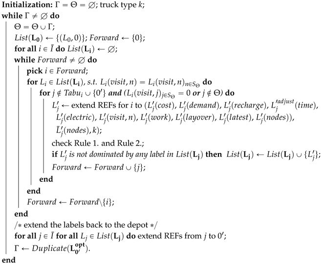
Recall that the resource L i ( v i s i t , n ) only stores the visiting information for “critical" shipments, i.e., the shipments visited more than once are marked as critical and the labeling algorithm repeats until all the optimal routes are elementary. The so-called decremental state-space relaxation (DSSR) was initially proposed by Righini and Salani (2008). Let Θ be the set of critical shipments found in the current iteration. Let Γ be the set of critical shipments in the optimal solutions discovered by the DSSR labeling algorithm, where non-elementarity is allowed. In each iteration, we update the set Θ by Θ = Γ Θ . This iteration procedure is repeated until the sets Γ becomes empty, and we reach an optimal solution for the ESPPRC. Algorithm 1 shows a generic version of this forward labeling algorithm for the pricing problem of MVRPC. L i s t ( L i ) is the list of forward states associated with node i. F o r w a r d is the set of nodes to be checked and extended. And S Θ is the set of critical shipments found up to the current iteration plus the unreachable nodes for each. The function D u p l i c a t e ( ) returns the set of nodes that cause the cycles in the current n optimal paths. The parameter n is set to 3 in our study.    
Algorithm 1:Bounded forward search with decremental state-space relaxation
Preprints 79742 i001

5.3. Bidirectional Labeling Algorithm

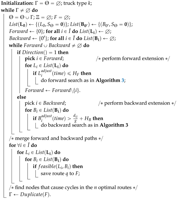
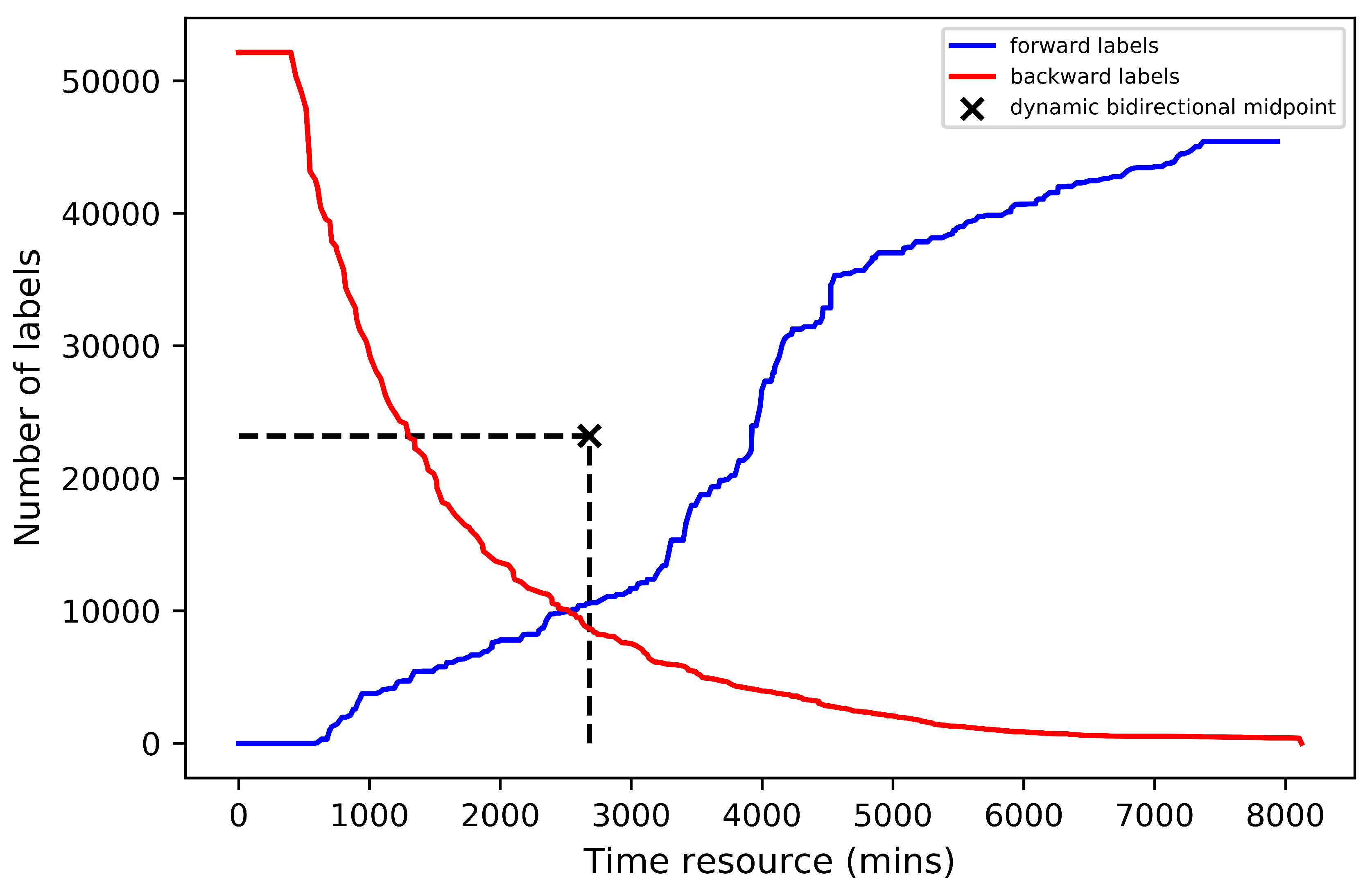
Bidirectional labeling algorithms are widely used in solving the pricing problems of VRP variants. They are especially beneficial in mitigating the explosion of labels, see Tilk et al. (2017). It has been observed in Righini and Salani (2006) and many more recent works that the bidirectional labeling algorithms are usually superior to their mono-directional counterparts and lead to substantially improved computational times for solving related SPPRC. When running a bidirectional algorithm, both forward partial paths and backward partial paths are created and extended alternatively. Each direction is processed up to a so-called “halfway point" (Righini and Salani (2006)). The halfway point is the midpoint of the domain of a monotone critical resource, e.g. L i ( t i m e ) for our case. Recall that along a partial path the time-related and load-related resources are all monotone. Along a forward path, the arrival times and the accumulated demands are non-decreasing. This standard bidirectional search mechanism with fixed halfway point has been adopted as almost a quasi-standard for solving ESPPRC. However, when it comes to renewable resources, such as EV recharging, Tilk et al. (2017) observed the number of forward and backward labels can differ significantly due to the fixed halfway point setting. Since MVRPC involves two renewable resources, i.e., EV recharging and replenishment layovers, we decide to adopt a dynamic halfway point scheme as in Tilk et al. (2017) to combat the potential unbalanced extensions. In our work, we choose to use time windows as the critical resource because it considers the layover resources and is more restrictive than the demand resource. In fact, the more restrictive the monotone resource is, the more effective is bidirectional labeling.
It is worth noting that the relaxed bounded bidirectional search with forward and backward propagations may result in either feasible or infeasible complete paths because of cycles. As can be seen from Figure 2, both forward and backward extensions can result in cyclic partial paths (top); even if the two partial paths are elementary, because certain shipments may occur in both paths, a cycle can be produced by joining them (e.g., shipment k in the bottom panel). This issue can be addressed by a modified DSSR feasible check, which will be discussed later.

5.3.1. Dynamic Halfway Points

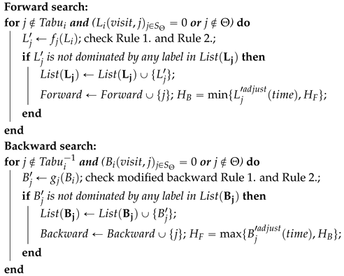
We start with the definitions of necessary components for the bidirectional search. The upper bound of the halfway point H F of the time resource is initialized as ( max i I { b i } + max i I ¯ { d i 0 g } + max i I { λ i } ) . H F is the halfway point for the forward search, which indicates half of the latest possible return time to the depot. Then, the forward search proceeds as in Algorithm 1 only if its L i a d j u s t ( t i m e ) does not pass the forward halfway point H F . As for the backward extension, the search direction is against the travel direction. The extension of the critical resource will be proceeded towards the lower bound of the halfway point H B , which is initialized as ( min i I { a i } + min i I ¯ { d i 0 g } + min i I { λ i } ) . Let B i a d j u s t ( t i m e ) be the adjusted backward time resource. Every time a forward label is extended, the backward halfway point H B is updated by the following rule to H B = min { L i a d j u s t ( t i m e ) , H F } . Alternatively, when a backward label is extended, the forward halfway point is updated to H F = max { B i a d j u s t ( t i m e ) , H B } . Note that the forward halfway point remains non-decreasing whereas the backward halfway point remains non-increasing. The two alternative updating steps ensure that H F H B , which guarantees the optimality. In addition, the initial values of H F and H B restrict the evolution of the dynamic halfway point to lie in the interval [ H F , H B ] . If we initialize H F = H B , then this becomes the standard fixed bidirectional labeling algorithm.

5.3.2. Backward Resource Extension Functions

Although the REFs for backward search are defined similar to the forward search, some adaptions need to be made. Consider a backward path traveled by an EV, q = ( i , . . . , e q . . . , 0 ) , that requires a visit to the recharger e q . Then, e q is named the “next recharger" of q, which implies there is no additional recharging visit between node i and e q . The amount of electricity consumed from i to e q varies while we extend the label backwards. We need an additional resource B i ( s l a c k ) for the sake of merging forward and backward labels. This resource is the maximum available recharging time for e q , assuming that all time windows along path ( j , 0 ) are respected. Moreover, whether the working hours hit the limit is unknown as well because it depends on the schedules from 0 to i, which are performed by the forward search. For a type-k backward path q = ( i , . . . , 0 ) , the label B i is defined by the following attributes: B i = ( B i ( c o s t ) , B i ( d e m a n d ) , B i ( r e c h a r g e ) , B i a d j u s t ( t i m e ) , B i ( e l e c t r i c ) , B i ( v i s i t , n ) , B i ( e l a p s e d ) , B i ( w o r k ) , B i ( l a y o v e r ) , B i ( l a t e s t ) , B i ( s l a c k ) , B i ( n o d e s ) ) , B ¯ i ( n o d e s ) , k ) . In order to use the similar REFs definitions as in forward labeling procedure, we need the following adaptions.
B i ( c o s t ) Reduced cost of partial path q.
B i ( d e m a n d ) Residual space on the truck, which equals to the accumulated
demand from 0 except at the last node i.
B i ( r e c h a r g e ) Negative number of recharges along path q except at node i.
B i ( t i m e ) Latest arrival time at i I ¯ 0 without breaking any time window.
B i ( e l e c t r i c ) Accumulated electricity consumption from 0 or a recharger back
to node i along the path q. Note this resource is renewable.
B i ( v i s i t , n ) A dummy resource variable that records the number of times any
critical shipment n S is visited along path q except node i.
Let the value be 1 if unreachable, which indicates
B i ( d e m a n d ) + ω i + ω n > Q k or B i ( t i m e ) d n i g λ n .
B i ( e l a p s e d ) Accumulated elapsed time (hours) from the next layover ( 0 if no
layover) to i.
B i ( w o r k ) Accumulated working time (hours) from the next layover ( 0 if no
layover) to i.
B i ( l a y o v e r ) Negative number of layovers the driver has taken from 0 to i.
B i ( l a t e s t ) The latest possible time to which the end of last layover period
can be extended to j without violating any resource constraint.
B i ( s l a c k ) Maximum flexible period that can be used for the next recharge
that satisfies the time windows while running EV on the path.
B i ( n o d e s ) A vector that stores the visited nodes along backward path q.
The backward labeling procedure starts from node 0 with the initial values assigned to each resource of B 0 , where B 0 ( t i m e ) = B 0 a d j u s t ( t i m e ) = b 0 , B 0 ( l a t e s t ) = a 0 , B 0 ( s l a c k ) = α · φ (and B 0 ( s l a c k ) = 0 if k V D ), and the other resources are all set to 0. REFs for B i ( c o s t ) , B i ( d e m a n d ) , B i ( v i s i t , n ) , B i ( e l e c t r i c ) , B i ( n o d e s ) are defined the same as L i ( c o s t ) , L i ( d e m a n d ) , L i ( v i s i t , n ) , L i ( e l e c t r i c ) , L i ( n o d e s ) . If the backward path is assigned by an ICV, then B i ( e l e c t r i c ) = δ i j = 0 , ( i , j ) A . Again, nodes are unreachable to the current label if and only if the time window and/or the truck capacity are violated. Δ i j is also the same as before except that we use B i ( w o r k ) to substitute L i ( w o r k ) in the forward labeling procedure. Other resources of a label B i along a backward arc ( i , j ) A are extended towards H B by the following REFs. Moreover, we introduce the feasible arcs list T a b u i 1 on the inverted network, follow the same logic as forward search. Details are elaborated in Section 5.4.1. Note that the extension will be proceeded from 0 backwards before ( B i a d j u s t ( t i m e ) d i j g ) hitting the lower bound of the halfway point H B .
B j ( t i m e ) = B i a d j u s t ( t i m e ) d i j g α · δ i j , if Δ i j = 0 and i E , B i a d j u s t ( t i m e ) d i j g λ i , if Δ i j = 0 and i I { 0 } , B i a d j u s t ( t i m e ) α δ i j | Δ i j | ξ · β l b d i j g , if Δ i j < 0 and i E , B i a d j u s t ( t i m e ) | Δ i j | ξ · β l b d i j g λ i , otherwise .
B j ( r e c h a r g e ) = B i ( r e c h a r g e ) 1 , if i E , 0 , otherwise .
B j ( s l a c k ) = B 0 ( s l a c k ) , if B i ( r e c h a r g e ) = 0 and i E , min { B 0 ( s l a c k ) α · δ i j , B j a d j u s t ( t i m e ) a j λ j } , if i E , min { B i ( s l a c k ) α · δ i j , B j a d j u s t ( t i m e ) a j λ j } , otherwise .
B j ( l a y o v e r ) = B i ( l a y o v e r ) 0 , if Δ i j = 0 , | Δ i j | ξ , otherwise .
B j ( e l a p s e d ) = B i ( e l a p s e d ) + α · δ i j + d i j g , if Δ i j = 0 and i E , B i ( e l a p s e d ) + d i j g + λ i , if Δ i j = 0 and i I { 0 } , B i ( w o r k ) + d i j g | Δ i j | ξ · ξ , if Δ i j < 0 and i E , B i ( w o r k ) + d i j g + λ i | Δ i j | ξ · ξ , otherwise .
B j ( w o r k ) = B i ( w o r k ) + d i j g + λ i , if Δ i j = 0 , B i ( w o r k ) + d i j g + λ i | Δ i j | ξ · ξ , otherwise .
B j ( l a t e s t ) = max { B i ( l a t e s t ) , B j ( e l a p s e d ) + a j + λ j } , if Δ i j = 0 , max { B j ( e l a p s e d ) + a j + λ j , B i ( l a t e s t ) B i ( e l a p s e d ) [ B i ( t i m e ) B j ( t i m e ) ] + B j ( e l a p s e d ) ( β u b β l b ) · | Δ i j | ξ } , otherwise .
REFs (59), (63)-(65) are similar to their forward counterparts, yet are propagated in an inverted direction. The unloading times at the current j are not taken into account in computing the resources. Furthermore, when the recharging activity happens right before a layover (in the reversed chronological order), the recharging time α · δ i j at recharger i should not be considered in the calculations of B j ( e l a p s e d ) . The reason is that this activity happened before the layover period and the truncated elapsed time should only track the driving and unloading time afterwards. When checking the time resource feasibility, each time window at shipment i will be shifted by λ i to [ a i + λ i , b i + λ i ] . Since the time windows for the rechargers are relaxed, a labeling extension to rechargers always satisfies the time window constraint. Moreover, even without any layover associated with a backward arc ( i , j ) , the current time B j ( t i m e ) , which may be greater than b j , can be adjusted to fit into the time window if and only if B j ( l a t e s t ) B j ( e l a p s e d ) b j + λ j . Therefore, the updated current time for the backward path is:
B j a d j u s t ( t i m e ) = min { B j ( t i m e ) , b j + λ j } .
The sequence of extending and checking the backward REFs are the same as discussed for the forward labeling procedure. The resulting label B i = ( B i ( c o s t ) , B i ( d e m a n d ) , B i ( r e c h a r g e ) , B i a d j u s t ( t i m e ) , B i ( e l e c t r i c ) , B i ( v i s i t , n ) , B i ( e l a p s e d ) ,
B i ( w o r k ) , B i ( l a y o v e r ) , B i ( l a t e s t ) , B i ( s l a c k ) , B i ( n o d e s ) ) , B ¯ i ( n o d e s ) , k ) is deemed feasible if B i ( d e m a n d ) Q k , a i B i a d j u s t ( t i m e ) λ i b i , B i ( s l a c k ) 0 , B i ( e l e c t r i c ) α · φ , and B i ( v i s i t , n ) 1 for all n S . If B i failed to pass any feasibility check, it is dropped. Now let us consider another straightforward example which shows the consistency and difference between forward and backward labeling.
Example 3. 
Figure 3 shows another complete EV route with a single visit to rechargers. The route is built by the backward extension. Other configurations are the same as Example 2 except for the parameter values. In this example, the route generated from the backward propagation can be exactly reproduced by the forward extension. However, the detailed schedules (arrival time and layovers) may or may not be different. This allows generation of diverse columns while keeping the number of labels lower than mono-directional searches. The aroused issues such as infeasible routes after merging the partial paths can be offset by the framework of dynamic halfway points.
The backward extension starts from the copy of depot 0 , then the extension follows the above-defined REFs and the depicted time windows, travel time, power consumption, and unloading time. After the first two extensions, this label arrives at node 1. The resource B 1 ( t i m e ) needs to be adjusted to fit in the time window. Also, the resource B 1 ( s l a c k ) is updated reflecting a minimum recharging of the power consumed on arc ( 1 , A ) . B 1 ( s l a c k ) indicates how much additional electricity can be assumed on the paths ahead, which have not yet been determined. The extension along arc ( 1 , A ) yields B 1 ( t i m e ) = 76 3 0.9 10 = 62.1 , B 1 ( e l e c t r i c ) = 0.03 × 30 = 0.9 , B 1 ( e l a p s e d ) = 12 + 3 14 = 1 = B 1 ( w o r k ) , B 1 ( s l a c k ) = 6 0.9 = 5.1 , B 1 ( l a t e s t ) = max { 30 + 1 + 4 , 58 12 13.9 + 1 4 } = 35 . This example illustrates how recharging time should be eliminated from the calculation B i ( e l a p s e d ) . In fact, recharging is not taken into account for the hours of service regulation and is only used for tracking the current time. Indeed, even if the recharge at A was additionally required for up to B 1 ( s l a c k ) = 5.1 units of time due to other possible extensions, B 1 ( t i m e ) would be set at 62.1 5.1 = 57 . The adjusted time would still fit into the time window, which is set at B a d j u s t = min { 57 , 54 } = 54 .
Preprints 79742 i005
To avoid explosion of backward labels, the two dominance rules introduced in Rule 1. and Rule 2. are still valid for the backward counterparts. The only difference is that certain non-decreasing monotone resources become non-increasing. To apply the two dominance rules, apart from changing all resources from L i s to B i s , we need the following adaptions. First, the signs of the time resource ( B i a d j u s t ( t i m e ) ), the number of recharges resource ( B i ( r e c h a r g e ) ), and the layover resource ( B i ( l a y o v e r )) are switched from ≤ to ≥. Also, the sign of B i ( l a t e s t ) is reversed from ≥ in forward search to ≤. Second, according to Desaulniers et al. (2016), all strictly negative values of B i ( r e c h a r g e ) are equally good. Therefore, REF (60) can be strengthened to B j ( r e c h a r g e ) = max { 1 , B i ( r e c h a r g e ) 1 } , if i E . Similarly, REF (62) for the layover resource can be strengthened in the same way to B j ( l a y o v e r ) = max { | Δ i j | ξ , B i ( l a y o v e r ) | Δ i j | ξ } , if Δ i j < 0 . Finally, the dominance criteria for the backward resource B i ( s l a c k ) is added, i.e., B i 1 ( s l a c k ) B i 2 ( s l a c k ) for label B i 2 dominated by label B i 1 .

5.3.3. Merge Forward and Backward Paths

In bidirectional labeling algorithms, labels are propagated to the halfway point. If either bound of the dynamic halfway point stays at the initial position, then a mono-directional labeling search is performed. Sometimes, it is also beneficial to make an adjustment such that more columns with negative reduced cost can be priced, although in the most cases halfway points are updated towards the middle of the critical resource. Once the forward labeling and the backward labeling extensions are completed, forward and backward labels are joined together at the halfway point to form complete paths. Suppose there are two labels L i and B i representing a forward and a backward path, respectively, ending at node i. Merging these two labels yields a complete origin to destination path with reduced cost L i ( c o s t ) + B i ( c o s t ) . The path is feasible if and only if the following conditions are fulfilled:
1.
L i ( v i s i t , n ) + B i ( v i s i t , n ) 1 , n S Θ , where S Θ is the set of critical shipments that maintain elementarity.
2.
The path respects the vehicle capacity: L i ( d e m a n d ) + B i ( d e m a n d ) Q k + ω i , k V .
3.
The path is feasible with respect to the time resource. The feasibility should be considered by two distinct cases.
Case 1. 
The backward path from i + 1 to 0 visits at least 1 recharger, i.e., B i ( r e c h a r g e ) < 0 , L i a d j u s t ( t i m e ) + L i ( e l e c t r i c ) + λ i B i a d j u s t ( t i m e ) , L i ( e l e c t r i c ) + B i ( e l e c t r i c ) α · φ , and L i ( e l e c t r i c ) B i ( s l a c k ) , L i ( l a t e s t ) + L i ( e l a p s e d ) B i a d j u s t ( t i m e ) λ i .
Case 2. 
The backward path from i + 1 to 0 visits no recharger, i.e.,
B i ( r e c h a r g e ) = 0 , L i a d j u s t ( t i m e ) B i a d j u s t ( t i m e ) λ i , L i ( e l e c t r i c ) + B i ( e l e c t r i c ) α · φ , and
L i ( l a t e s t ) + L i ( e l a p s e d ) B i a d j u s t ( t i m e ) λ i .
4.
The accumulated working time does not break the hours of service regulation: L i ( w o r k ) + B i ( w o r k ) ξ .
After the merge, we perform a final dominance test with Rule 1. and Rule 2. for all merged routes. The non-dominated routes with negative reduced cost are candidate columns for the RMP.

5.3.4. Generic Structure of the Algorithm

The bidirectional labeling algorithm updates the two bounds of the halfway points towards each other. Apart from the extension mechanism introduced in the previous sections, it is important to determine criteria for how to alternate between forward and backward labeling so that the overall performance of the algorithm can be guaranteed. An ideal strategy is to choose the direction which may minimize the overall computational time. Tilk et al. (2017) suggest that a heuristic be added by choosing the direction with smaller number of already generated labels. This heuristic is also added in a function of our algorithm, which is named D i r e c t i o n ( ) . D i r e c t i o n ( ) = 1 if it chooses to do a forward extension. Otherwise, D i r e c t i o n ( ) = 0 . However, purely relying on this simple heuristic may cause too many infeasible merges. To overcome the issue, we collect L i and B i that are produced in the current iteration, such that no merge is possible for those labels, and store them into a list Ξ . After finishing the procedures of merge and feasibility check, the algorithm will extend the labels from Ξ in a monotone direction until they approach the depot (0 for backward and 0 for forward). In particular, if infeasibility has arisen due to the violation of service hour regulation, we continue forward extension from this state in the following iterations. For simplicity, we denote the operations for the forward REFs (45)-(58) as f j ( L i ) and the corresponding operations for the backward REFs as g j ( B i ) . Let f e a s i b l e ( L i , B i ) equal 1 if the merge of a forward and a backward label at node i passes all the conditions, and equals 0 otherwise. Once a complete route is merged, we store the feasible route q in a set F. The selected routes in F with negative reduced cost will finally be passed to Ω in the RMP. With these additional notations, the bounded bidirectional labeling framework is given in Algorithm 2. The forward and backward functions are shown in Algorithm 3.    
Algorithm 2:Bounded bidirectional labeling algorithm
Preprints 79742 i002
Algorithm 3:Forward and backward search steps
Preprints 79742 i003

5.4. Implementation Strategies

5.4.1. Preprocessing and Candidate List

The search space of MVPRC is extremely large. Therefore, preprocessing controlling the feasible arcs is an effective way to improve the algorithmic performance. First, as in Section 3.2, any visit to electric rechargers through an ICV is defined infeasible. The associated variables are set to 0. Also, we allow no consecutive visits to rechargers, i.e., ( i , j , e ) = 0 , i , j E . Second, due to the truck capacity constraint, shipments that cannot be fit on the same truck k are pivoted. Third, the intra-node distance constraint (18) detects the infeasible arc combinations. Next, we preprocess the nodes that cannot be fit into the same time windows. For example, suppose shipment 1 is restricted to be delivered within time interval [ 0 , 10 ] and shipment 2 is within [ 35 , 50 ] . Since the difference is more than the longest layover period, there is no feasible arc ( i , j , k ) on the network. Furthermore, shipments with a lower common carrier cost m i than the stop cost p are deemed to be outsourced. Based on the above conditions, we preprocess the graph before the column generation framework. For each node i, we create a candidate list which stores all the nodes that can be directly linked to i without violating any of the above conditions. Conversely, for nodes that cannot be visited by i that are specified by the conditions, we store them in a forbidden list called T a b u i . Similarly, we define the forbidden list T a b u i 1 for backward search by subtracting and checking the resources.

5.4.2. Heuristic Pricing Procedure

To speed up the generation of dedicated fleet paths with negative reduced cost, we first employ a simple heuristic procedure. The two developed exact labeling algorithms are implemented only if the heuristic procedure stops generating paths with negative reduced cost. This procedure has two steps. Firstly, for each node i I ¯ , we reduce the search space by allowing only the extension from i to ρ nodes with the smallest arc reduced cost c ¯ i j k . In this way, at most ρ · ( n + m ) REF operations can be performed in each iteration. Whenever the first step fails, the number of candidate nodes are enlarged to 2 ρ and then to 3 ρ . Secondly, we set a limit to the number of labels kept along the label extensions. For example, we can start with allowing only 500 labels to be stored in L i s t ( ) and then increase the number to 1000 if 500 failed to generate paths with negative reduced costs, and so on.

5.4.3. 2-cycle Elimination

As our relaxed labeling algorithm allows cycles to exist in the extension steps, non-elementary paths contain a cycle of the form ( i , j , i ) , e.g. ( 0 , 1 , 2 , 1 , 3 , 0 ) . These cycles are known as 2-cycles and are the most frequently occurring type of cycle caused by DP-based approaches (Desrochers et al. (1992)). When extending labels as shown in Algorithm 1 and Algorithm 2, we apply the 2-cycle elimination procedure introduced by Desrochers et al. (1992). The basic idea is to keep the best and the second-best partial paths for each state i and re-evaluate the new cost of extending i to j complying with the resources. The value of j is determined by two conditions, one is set to i’s predecessor,the other is not. We add the predecessor to S Θ and updated this value on a rolling-basis.
Recall that we use the relaxed state space Θ in the backward and forward labeling algorithm to keep track of the critical shipments. This technique drastically reduces the number of states required to be explored. However, this manipulation introduces cycles in the generated solutions. Goel and Irnich (2014) have computed the minimum mandatory layover and break periods between two customers. Here, we discover another way to expand set Θ based on an approximate lower bound of the layovers. More specifically, a 2-cycle of the form ( i , j , i ) may be possible if max { a i + ( d 0 i g + λ i ) ξ · β l b , a j } + ( d 0 i g + λ i ) ξ · β l b b i . We check each pair i , j I ¯ with this inequality before calling the algorithm, each time an arc ( i , j ) is valid, we add node i to Θ to ensure elementarity along the path.

5.5. Modified Dominance Criteria

Consider the dedicated fleet pricing problem of the format (41). Recall that the 2-path inequality and the multistar inequality are both robust, The reduced cost changed by adding them to the RMP can be decomposed by arcs on the subproblem network, as shown in (42). However, applying the SR inequality interrupts the search space and the feasibility of the generated columns, see Jepsen et al. (2008). The dominance criteria developed in Rule 1. and Rule 2. are no longer valid. The two rules need to be modified to capture the dual values invoked by the SR inequality (35). During the execution of the modified algorithm, we need only to consider non-dominated paths.
By solving the separation problem (38), we get a SR inequality (35) with the modified reduced cost shown in (43). Set S I is of cardinality three and 0 < ϕ ω ( S ) . Using the notations of labels, we can express the coefficient of the dual value χ r applied on the current partial path by ω ( S L i ( n o d e s ) ) ϕ . Then, the first improvement on the two dominance criteria is produced by substituting the conditions L i 1 ( n o d e s ) L i 2 ( n o d e s ) and L i 1 ( v i s i t , n ) L i 2 ( v i s i t , n ) by L ¯ i 1 ( n o d e s ) L ¯ i 2 ( n o d e s ) . In fact, this means the possible space of extensions for label L 1 is larger than that for label L 2 . As further cuts are identified and added, Rule 1. and Rule 2. will not be effective as in the initial stage because penalties had already been imposed. Therefore, rare conditions in the two rules are satisfied. In order to overcome this problem, we note the following property of (43).
c ˜ q = c ^ q ω ( S L i ( n o d e s ) ) ϕ · χ r = c ˜ q ω ( S L i ( n o d e s ) ) mod ϕ · χ r .
Therefore, we define m ( L i ) = ω ( S L i ( n o d e s ) ) mod ϕ after the last dual penalty has been applied on the reduced cost by delivering ϕ demands through set S. In the case that L i 1 dominates L i 2 , L i 1 ( c o s t ) L i 2 ( c o s t ) , and ω ( S L i 1 ( n o d e s ) ω ( S L i 2 ( n o d e s ) . Thus, L i 1 ( c ˜ ) L i 2 ( c ˜ ) , given χ r < 0 . Only demands after the last penalty towards the target node will be affected, see Jepsen et al. (2008). Considering two labels L 1 and L 2 , then the larger the m ( L i ) , the sooner will the corresponding label incur another penalty to the reduced cost. We define the following set:
M ( L i 1 , L i 2 ) = { S S E P : m ( L i 1 ) > m ( L i 2 ) } .
where S E P denotes combinations of the set S found by the separation optimization that induce active SR inequality (35). The dominance criterion Rule 1. can be strengthened to:
Proposition 5.3 
(Rule 3.). Define two labels L 1 and L 2 associated with the same node i. Then, label L i 2 is dominated by label L i 1 only if all the following conditions are satisfied and at least one of the inequalities is strict. Therefore, L i 2 can be discarded. L i q ( c ˜ ) denotes the modified reduced cost of label q imposed with SR inequalities.
i I ¯ 0 { 0 } L ¯ i 1 ( n o d e s ) L ¯ i 2 ( n o d e s ) , L i 1 ( d e m a n d ) L i 2 ( d e m a n d ) L i 1 , a d j u s t ( t i m e ) L i 2 , a d j u s t ( t i m e ) , L i 1 ( w o r k ) L i 2 ( w o r k ) , L i 1 ( e l e c t r i c ) L i 2 ( e l e c t r i c ) , L i 1 ( r e c h a r g e ) L i 2 ( r e c h a r g e ) , L i 1 ( l a y o v e r ) L i 2 ( l a y o v e r ) , L i 1 ( l a t e s t ) L i 2 ( l a t e s t ) L i 1 ( c ˜ ) M ( L i 1 , L i 2 ) χ r L i 2 ( c ˜ ) .
Proof. Consider any possible extension L j 2 L ¯ i 2 . Because for any S M ( L i 1 , L i 2 ) we have m ( L i 1 ) > m ( L i 2 ) , the future coefficients for the dual variables maintain the following relationship.
ω ( S L j 2 ( n o d e s ) ) + m ( L i 1 ) ϕ ω ( S L j 2 ( n o d e s ) ) + m ( L i 2 ) ϕ .
Since 0 m ( L i 2 ) < m ( L i 1 ) ϕ , the left-hand side of 69 is at most one unit larger than the right-hand side, which means label L 1 can conduct at most one more χ r penalty to the reduced cost than L 2 . This lead to:
ω ( S L j 2 ( n o d e s ) ) + m ( L i 1 ) ϕ 1 ω ( S L j 2 ( n o d e s ) ) + m ( L i 2 ) ϕ .
Therefore, we have:
L j 1 ( c ˜ ) = L i 1 ( c ˜ ) + c ^ i j k ω ( S L j 2 ( n o d e s ) ) + m ( L i 1 ) ϕ · χ r L j 1 ( c ˜ ) = L i 1 ( c ˜ ) χ r + c ^ i j k ( ω ( S L j 2 ( n o d e s ) ) + m ( L i 1 ) ϕ 1 ) · χ r L j 1 ( c ˜ ) L i 2 ( c ˜ ) + c ^ i j k ω ( S L j 2 ( n o d e s ) ) + m ( L i 2 ) ϕ · χ r L j 1 ( c ˜ ) = L j 2 ( c ˜ ) .
Because we allow multiple SR inequalities to be added in a single iteration, this indicates L i 1 ( c ˜ ) M ( L i 1 , L i 2 ) χ r L i 2 ( c ˜ ) is satisfied. The other conditions are ensured by Rule 1. Hence, label L 2 is dominated by label L 1 . □
By similar adjustment of Rule 2. we can reach a modified dominance criteria Rule 4.

5.6. Branching Rules

When the subproblem does not pass any columns with negative reduced cost to the RMP, the LP solver provides us the optimal solution for the linear relaxation of the set partitioning reformulation. If the solution is integer and all the constraints are respected, this solution is also optimal for MVRPC. Otherwise, the solution is fractional and a branch-and-bound tree must be explored. Additional columns could be generated at each branch. In our implementation, we refer to the best-bound strategy used by Desrochers et al. (1992) and Dabia et al. (2019,a). Note that all the branching decisions are made based on the arc-flow formulation ( P ) . The variables are projected by equation (25). The branching strategy can be separated into multiple levels: (i) we start with branching on the outsourcing decision variable y i . The algorithm finds the y i that is closest to 0.5 in each iteration and creates two branches y i 0 and y i 1 . When the variables y i are integers for all i I , we proceed to the next level of branching. (ii) The algorithm branches on the number of vehicles k V i I ¯ x 0 i k over all vehicle types and sizes. Two branches are created, k V i I ¯ x 0 i k k V i I ¯ x 0 i k L P and k V i I ¯ x 0 i k k V i I ¯ x 0 i k L P , where x L P is the optimal fractional solution at the current branch. (iii) If the number of total vehicles is an integer, then we decide to branch on the number of routes per truck type k. We choose the truck type k for which the fractional part of the number is closest to 0.5. Thereafter, a branch is created, i I ¯ x 0 i k i I ¯ x 0 i k L P and i I ¯ x 0 i k i I ¯ x 0 i k L P . (iv) If the previous two numbers are both integers, we start branching on the number of recharges. First, we choose to branch on the fractional portion of the total number of visits to i E that closest to 0.5. Then, a branch on each location of the recharger is created follow the same logic. For every branch created up to this stage, the decision is imposed by adding the associated inequality to the RMP. The corresponding dual values of the added inequality need to be transferred to the reduced cost of the related columns. Each time the past four branching strategies are utilized, the current solution is no longer feasible, which means a reoptimization is required on the linear relaxation.
Next, branching decisions are taken on the arcs of the subproblem network. (v) we check the pair of ( i , j , k ) A such that x i j k L P + x j i k L P is closest to 0.5, and imposes two branches x i j k + x j i k 0 and x i j k + x j i k 1 . (v) Finally, among all arcs ( i , j , k ) with a fractional value in the current solution, we choose several x i j k L P close to 0.5. Ties are broken by preferring arcs with higher cost c ¯ i j k . Incident arcs to j on vehicle k are removed temporarily from the graph G if x i j k L P is set to 1. The branch-and-bound tree is enumerated according to the impact of the branching decisions on the two child nodes of the candidates. In other words, each time we reoptimize the RMP, the increase of the lower bounds of the two child nodes are measured, and the maximum is chosen as the next move. The number of branch candidates is set as 20 in our study. We adopt the hybrid search technique used by Desaulniers et al. (2016), in which subtrees will be explored only if their father nodes’ lower bound is within a gap of ε of the current best lower bound.
This process is repeated until the entire search tree is explored.

6. Computational Results

In this section, we present computational experiments to analyze the effectiveness of the proposed branch-and-cut-and-price algorithm and to assess the impacts of allowing mixed type vehicle fleets and outsourcing options. Section 6.1 describes the instance and parameter settings used in our study. All algorithms are implemented in Python 3.8 on an Intel Core i9 CPU, 2.3 GHz 8-Core, 16 GB of RAM. For all experiments, we use a time limit of 2 hours. The LP relaxation of the master problem is solved using commercial solver Gurobi 9.0.

6.1. Parameter Settings

The benchmark set for MVRPC is the same as introduced in Dang et al. (2020), where the 11 instances are provided by DHL Supply Chain. We apply the following modifications to obtain MVRPC instances: 1) 40 selected rechargers are deployed to several warehouse locations; 2) the battery capacity of the electric vehicles, energy consumption, and other parameters are set by the medium configurations of Tesla’s Semi truck, see Tesla Motors Inc. (2020); 3) Instances S 1 , S 2 and S 5 shown in Table 1 are directly tested, while we randomly generate another three instances of 80, 120, and 150 customers from instance M 0 and M 1 ; 4) Other route-related parameters and parameters for the trucks are shown in Table 3 and Table 4, respectively. Note that the fixed cost per day of each truck type is estimated by the purchase cost divided by 7-year asset depreciation with 260 yearly working days. This estimation is an industry convention provided by experienced transportation analysts. For the cost of outsourcing, we again use the tariff sheets depending on the geographical location of the customers. For simplicity, we access the tariff in advance and assign the common carrier cost for each shipment. For all instances, we set the number of available vehicles to be five for the four truck types. At any point during the search, we limit the number of active valid inequalities to be 100. An initial upper bound of the problem is determined by the cost of outsourcing all shipments.

6.2. Algorithmic Performance

First, we study the performances of the MILP formulation and our branch-and-cut-and-price algorithms. Impacts of the three sets of valid inequalities are compared between robust and non-robust categories. A valid inequality is generated when it is violated by more than 0.2. The heuristic pricing procedures introduced in Section 5.4 are called to speed up the procedure of finding the routes with negative reduced cost. The number of labels stored in the L i s t ( ) is updated by increasing the number of labels by 500 each time we call the pricing problem. At most three of the routes for each vehicle type with the negative reduced costs are added to the RMP in the same pricing iteration.
Table 5 shows the results over the six instances by the branch-and-cut solver using our MILP formulation and the BCP algorithms with different valid inequalities. The first setting of the BCP is to disable the cutting planes so that a branch-and-price method is utilized. Based on the analytical results in Section 4.1, we decide to combine the 2-path inequalities and the generalized large multistar inequalities together because they are both developed based on the arc-flow formulation and are thus robust inequalities. Next, SR inequalities are applied to the current BCP algorithm to test the effectiveness of the CG rank-1 cuts. In Table 5, The sizes of the instances are given in the column named Instances, (e.g., S1-N25 indicates instance S1 has 25 shipments). The time in seconds indicates when the instances are solved to proven optimality within the time limit 7200 seconds. In the following columns, the number of branch-and-bound nodes explored in the master problem (Nodes) and the relative integrality gap between upper and lower bounds (Gap (%)) are reported. The relative gap is computed as z I P z L P z I P , where z I P and z L P are the optimal values of the integer solution and the linear relaxation. For instances that are not solved to optimality within the two-hour limit, we report the final gaps.
We see that MILP formulation is not competitive even for the modest-size instances, which were also observed in previous works for other VRP variants. The main reason is that the LP relaxation bound of ( P ) is so weak that a large number of nodes needs to be explored to prove optimality. The branch-and-price method without applying any cutting plane is able to solve four out of the six instances and yields a small optimality gap for the two large instances that are not solved within the time limit. The BCP method with the two robust valid inequalities solves the same number of instances as the method without the cuts, however, the run time is decreased and the final gaps are reduced for the two large-sized, which means the two sets of cuts are effective. When the SR inequalities are separated and applied to the BCP algorithm, the run time reduction is more obvious. One more instance M1-N120 with 120 shipments can be solved to optimality within the two-hour limit. Compared with the two robust inequalities, SR inequality outperforms the other two and has the biggest influence on improving the lower bounds. Finally, we observe that the number of nodes fathomed is very small compared with the MILP solver, and the root optimality gap is close to 0 for those solved instances.
Second, we investigate the performance of the branch-and-cut-and-price algorithms with forward and bidirectional labeling procedures for MVRPC. We compare the performance of the forward labeling and the bidirectional labeling algorithms. The heuristic pricing procedures are used in this experiment. Table 6 gives results for the four small-sized instances. For each labeling algorithm, the table contains the time spent on the pricing problem in seconds, the number of labels generated during the iterations, and the number of pricing problem iterations needed. A single pricing problem iteration is completed when the optimal routes are passed to the RMP to get the new LP solution.
The results of this test show that the bidirectional labeling algorithm is superior to the mono-directional version. The solution by bidirectional search of a single instance takes on average over one third the time forward search needs. The number of labels generated in total deceased by nearly half by utilizing the bidirectional method. However, we notice that the average number of pricing problem iterations needed to solve a single instance is nearly identical for both versions. By subtracting the solution time shown in Table 5 by the times spent in the pricing problems shown in Table 6, we have an interesting finding. Most of the solution time is spent on strong branching, but in most cases, strong branching does help to keep the size of the branch-and-bound tree small.
Figure 4 shows an example of the accumulated labels generated by the three labeling directions, i.e., forward, backward, and bi-directional. This example indicates that the mono-directional labeling algorithms generate about twice the labels of the bidirectional method. In fact, at the dynamic halfway point, the bidirectional labeling algorithm merges the forward and backward labels. Recall that, for labels that cannot be merged from either direction, we extend the labels crossing the halfway point until the depot (0 or 0 ).

6.3. Sensitivity Analyses on Recharging and Outsourcing

By closely looking into the structure of the optimal solutions visualized in the figures, we can derive some insights by conducting a few sensitivity analyses.
To start, we investigate the impact of the vehicle fixed cost and the battery capacity. Recall that different from the previous works, MVRPC considers an accumulated daily usage cost of the trucks, which means the fixed vehicle cost may affect the solution structures because more layovers imply higher truck usage cost. While Tesla’s Semi truck is still a protocol, BYD’s 8TT has already been implemented in the market. The parameters of an electric tractor are: 40,000 lbs weight capacity, 409 kwh battery capacity, 2.6 kw/mile of EV power consumption, and fixed cost per day of $ 209 . The energy cost per mile is still set as the electric cost divided by mileage, which is $ 0.1 / m i l e . Figure 5 shows the optimal solutions of instance M0-N80 where the left panel (??) with the EV settings is shown in Table 4 and the right panel (??) with the EV settings as BYD’s 8TT. Clearly, customers located in more remote areas tend to be outsourced. Moreover, these customers either have relatively smaller demands or lower common carrier costs than shipping with the dedicated fleet. When the EV cost increases, it is expected that more shipments are served by either ICVs or common carriers. However, due to the battery capacity deduction, we observed in Figure 5 ICV routes and common carriers covered all the shipments while the BYD’s 8TT is introduced to the mixed fleet, which has cheaper daily usage cost. Moreover, the solution time is reduced by more than 35% together with a 5% cost increase. This is due to the decrease of battery power caused by less feasible EV routes. In other words, the algorithm does not need to consider selecting and scheduling over the 40 rechargers and thus reduces the solution time. But in general, we observed most instances are sensitive to the change of EV daily usage cost.
Figure 6 shows a comparison between deploying random-generated rechargers and the cherry-picked locations. Clearly, since the recharger locations are not well-designed, the optimal solution shown in Figure 6 does not utilize any EV route. In fact, the longer distance caused by visiting a recharger result in inefficient EV routes or infeasible EV paths due to tight time windows and possible layover periods. However, when we deploy the rechargers at or near to the customers’ warehouses, three ICV routes are substituted by EV routes to optimize the network costs.
Next, we investigate the impact of the outsourcing option. We discuss the impact of outsourcing on the structure of the optimal routes. We look at the solution by disabling the outsourcing option for instance M0-N80. Other parameters are set to be the same as in Figure ??. In this case, all shipments must be delivered by the mixed fleet. Compared with the optimal solution with an outsourcing option, the solution provided in Figure 7 results in 30% higher objective values. Furthermore, by outsourcing some customers, better routes with fewer trucks carrying a single or two shipments can be established. This might be due to the exclusion of uneconomical deliveries such that their time windows are tight or their locations are far away from the depot.

7. Conclusions and Future Works

In this paper, we presented the first exact approach for the MVRPC, which is a new variant of the vehicle routing problem with common carriers researched in the literature. New features are included to solve the question with heterogeneous fleet sizes, flexible layover periods, and the electric vehicle recharges. This is the first exact approach designed for the mixed fleet routing and mode decision problem.
The exact algorithm is based on the branch-and-cut-and-price framework. We provide a MILP formulation for the problem. Since the arc-flow MILP is usually not efficient in solving large-scale cases, we define an extensive set-partitioning reformulation for column generation. In this reformulation, variables for the fleet routes are considered to be further established in the subproblem pricing procedures, whereas the outsourcing decisions are made in the master problem. The performance of the algorithm is enhanced by using three sets of valid inequalities. To efficiently solve the subproblem, we designed new bounded labeling algorithms that successfully combine the idea of decremental state space relaxation and the dynamic halfway points. Mono-directional and bidirectional labeling algorithms for generating feasible routes are presented. Their efficiency results from tailored REFs that allow for time adjustments, renewable resources tracking, and strong dominance rules. Efficient implementation strategies were introduced to speed up the solution process.
In numerical studies, we demonstrate that our algorithms are capable of solving real-world instances with up to 120 customers and 40 rechargers. In addition, we show that the special case of CG rank-1 cuts – subrow inequality is more effective in cutting off fractional solutions than the other two developed valid inequalities based on arc-flow variables. Moreover, we show that, especially for large instances, the bidirectional labeling is superior compared to the mono-directional one. The time savings are mainly due to the reduction in the number of labels.
As this is the first exact algorithm for this variant of problems, there is apparently room for some improvement and future research. First, we notice that the main run time of the BCP algorithms are in the strong branching. Applying new branching techniques, e.g. see Alvarez et al. (2017), would be strongly beneficial to improve the performance of the algorithm. Second, different recharging policies, like partial recharging, non-linear power consumption, and different recharger costs/schedules, can be applied to the problem, leading to more complex models and solutions.

References

  1. Alcaraz J, Caballero-Arnaldos, Vales-Alonso (2019) Rich vehicle routing problem with last-mile outsourcing decisions. Transportation Research Part E, 129:263-286. [CrossRef]
  2. Alvarez AM, Louveaux Q, Wehenkel L (2017) A machine learning-based approximation of strong branching. INFORMS Journal on Computing, 2017 Feb;29(1):185-95. [CrossRef]
  3. Andelmin J, Bartolini E (2017) An Exact Algorithm for the Green Vehicle Routing Problem. Transportation Science, 51(4):1288-, 1303. [CrossRef]
  4. Arasu M., T. , Anwar H, Ahmed Q, Rizzoni G (2019) Energy Optimal Routing of a Delivery Vehicle Fleet With Diverse Powertrains. Proceedings of the ASME 2019 Dynamic Systems and Control Conference 1:Park City, Utah, USA. October 8–11, 2019. [CrossRef]
  5. Asghari M, Alehashem M (2020) Green vehicle routing problem: A state-of-the-art review. International Journal of Production Economics. [CrossRef]
  6. Baldacci R, Mingozzi A, Roberti R (2011) New route relaxation and pricing strategies for the vehicle routing problem. Operations Research, 59(5):1269-1283. [CrossRef]
  7. Chu C-W (2005) A heuristic algorithm for the truckload and less-than-truck-load problemEuro. Jo. Oper. Res. 165(3):657-667. [CrossRef]
  8. Chvátal V (1973) Edmonds polytopes and hierarchy of combinatorial problems. Discrete Mathematics, 4(4):305-337. [CrossRef]
  9. Conforti M, Cornuejols G, Zambelli G (2014) Integer Programming Chapter 5.1-5.3: 195-222, 1st Edition, Springer.
  10. Conrad, R.G. and Figliozzi M. A. ( 2011). The recharging vehicle routing problem. In Proceedings of the 2011 industrial engineering research conference (p. 8). IISE Norcross, GA.
  11. Dabia S, Lai D, Vigo D (2019) An exact alogirhm for a rich vehicle routing problem with private fleet and common carrier. Transportation Science, 53(4):986-1000. [CrossRef]
  12. Dabia S, Ropke S, Woensel T (2019) Cover Inequalities for a Vehicle Routing Problem with Time Windows and Shifts. Transportation Science, 53(5):1354-1371. [CrossRef]
  13. Dang Y, Singh M, Allen T (2020) Network mode optimization for the DHL Supply Chain. INFORMS Journal On Applied Analytics. [CrossRef]
  14. Demir E, Bektas T, Laporte G (2012). An adaptive large neighborhood search heuristic for the pollution-routing problem. European Journal of Operational Research, 223(2), 346–359. [CrossRef]
  15. Desaulniers G, Errico F, Irnich S, Schneider M (2016) Exact algorithms for electric vehicle-routing problems with time windows. Operations Research, 64(6): 1388–1405. [CrossRef]
  16. Desaulniers G, Desrosiers J, Ioachim I, Solomon M. M., Soumis F, Villeneuve D (1998) A unified framework for deterministic time constrained vehicle routing and crew scheduling problems. T. Crainic, & G. Laporte (Eds.), Fleet management and logistics 57–93. Boston, Dordrecht, London: Kluwer Academic Publisher.
  17. Desaulniers G, Lessard F, Hadjar A (2008) Tabu search, partial elementarity, and generalized k-path inequalities for the vehicle routing problem with time windows. Transportation Science, 42(3):387-404. [CrossRef]
  18. Desrochers M, Desrosiers J, Solomon M (1992) A new optimization algorithm for the vehicle routing problem with time windows. Operations Research, 40(2):342-354. [CrossRef]
  19. Dror M (1994) Improvements and extensions to the Miller-Tucker-zemlin subtour elimination constraints. Operations Research, 42:977-978. [CrossRef]
  20. DHL GoGreen Program (2020) Mission 2050: zero emissions. URL: https://www.dpdhl.com/en/sustainability/environment-and-solutions/gogreen-program. Accessed: 09/23/2020.
  21. Desrochers M, Laporte G (1991) Note on the complexity of the shortest path mod- els for column generation in VRPTW. Operations Research Letters, 10:27-36. [CrossRef]
  22. Federal Motor Carrier Safety Administration (2011) Hours of service of drivers. Federal Register. Vol. 76, No. 248, page 81134-81188.
  23. Feillet D, Dejax P, Gendreau M, Gueguen C (2004) An exact algorithm for the elementary shortest path problem with resource constraints: Application to some vehicle routing problems. Networks, 44(3):216-229. [CrossRef]
  24. Fischetti M, Lodi A (2007) Optimizing over the first Chavátal closure Math. Program. Ser. B 110:3-20.
  25. Fukasawa R, Longo H, Lysgaard J, Poggi de Aragao M, Reis M, Uchoa E, and Werneck RF (2006) Robust branch-and-cut-and-price for the capacitated vehicle routing problem. Math. Program. 106 (3):491-511.
  26. Fukasawa R, He Q, Song Y (2016) A branch-cut-and-price algorithm for the energy minimization vehicle routing problem. Transportation Science, 50(1):23-34. [CrossRef]
  27. Gahm C, Brabander C, Tuma A (2017) Vehicle routing problem with private fleet, multiple common carriers offering volume discounts, and rental options. Transportation Res. Part E. 97(C):192-216. [CrossRef]
  28. Goeke D, Schneider M (2015) Routing a mixed fleet of electric and conventional vehicles. European Journal of Operational Research, 245:81-99. [CrossRef]
  29. Goel A and Irnich S (2014) An exact method for vehicle routing and truck driver scheduling problems. Technical Report No. 33, Jacobs University, School of Engineering and Science, Bremen, Germany. [CrossRef]
  30. Gomory RE (1958) Outline of an algorithm for integer solutions to linear programs Bull AMS 64:275-258.
  31. Lübbecke M, Desrosiers J (2005) Selected topics in column generation. Operations Research, 53(6):1007–1023. [CrossRef]
  32. Irnich S, Desaulniers G (2005) Shortest path problems with resource constraints. Desaulniers G, Desrosiers J, Solomon M, eds. Column Generation (Springer, New York): 33–65.
  33. Irnich S, Villeneuve D (2006) The shortest path problem with resource constraints and k-cycle elimination for k≥3. INFORMS Journal on Computing, 18(3):391-406. [CrossRef]
  34. Jepsen M, Petersen B, Spoorendonk S, Pisinger D (2008) Subset-row inequalities applied to the vehicle routing problem with time windows. Operations Research, 56(2):497-511. [CrossRef]
  35. Kallehauge B (2008) Formulations and exact algorithms for the vehicle routing problem with time windows. it Comput. Oper. Res. 35(7):2307–2330. [CrossRef]
  36. Kohl N, Desrosiers J, Madsen OBG, Solomon MM, Soumis F (1999) 2-path cuts for the vehicle routing problem with time window. Transportation Science, 33(1):101-116. [CrossRef]
  37. Laporte G (2007) What you should know about the vehicle routing problem. Naval Res. Logist. 54(8):811-819. [CrossRef]
  38. Letchford AN, Eglese RW, Lysgaard J (2002) Multistars partial multistars and the capacitated vehicle routing problem. Math. Program. 94:21-40.
  39. Lübbecke, M.E. , Desrosiers J (2005) Selected Topics in Column Generation. Operations Research, 53(6):1007-1023. [CrossRef]
  40. Macrina G, Pugliese L.D.P., Guerriero, F, Laporte, G (2019) The green mixed fleet vehicle routing problem with partial battery recharging and time windows. Computers and Operations Research, 101:183-199. [CrossRef]
  41. Moon I, Lee JH, Seong J (2012) Vehicle routing problem with time windows considering overtime and outsourcing vehicles. Expert Syst. Appl. 39(18):13202–13213. [CrossRef]
  42. Pelletier S, Jabali O, Laporte G (2016) 50th anniversary invited article— Goods distribution with electric vehicles: Review and research per- spectives. Transportation Sience, 50(1): 3-22.
  43. Petersen, B. , Pisinger D., Spoorendonk S. (2008) Chvátal-Gomory Rank-1 Cuts Used in a Dantzig-Wolfe Decomposition of the Vehicle Routing Problem with Time Windows. In: Golden B., Raghavan S., Wasil E. (eds) The Vehicle Routing Problem: Latest Advances and New Challenges. Operations Research/Computer Science Interfaces, vol 43. Springer, Boston, MA.
  44. Righini G, Salani M (2006) Symmetry helps: bounded bi-directional dynamic programming for the elementary shortest path problem with resource constraints. Discrete Optim. 3(3):255–273. [CrossRef]
  45. Righini G, Salani M (2008) New dynamic programming algorithms for the resource constrained shortest path problem. Networks, 51(3):155-170. [CrossRef]
  46. Rousseaua LM, Gendreaub M, Feilletc D (2007) Interior point stabilization for column generation. Operations Research Letters, 35:660-668. [CrossRef]
  47. Schneider M, Stenger C, Goeke D (2014) The Electric Vehicle-Routing Problem with Time Windows and Recharging Stations. Transportation Science, 48(4): 500-520. [CrossRef]
  48. Semi-trailer, Wikipedia (2020) Electric Truck. URL: https://en.wikipedia.org/wiki/Electric truck. Accessed: 09/15/2020.
  49. Tesla Motors Inc. (2020) Supercharger. URL: https://www.tesla.com/supercharger. Accessed: 09/23/2020.
  50. Tilk C (2016) Branch-and-Price-and-Cut for the Vehicle Routing and Truck Driver Scheduling Problem. Working Papers 1616, Gutenberg School of Management and Economics, Johannes Gutenberg-Universität Mainz.
  51. Tilk C, Rothenbächer A, Gschwind T, Irnich S (2017) Asymmetry matters: Dynamic half-way points in bidirectional labeling for solving shortest path problems with resource constraints faster. European Journal of Operational Research, 261: 530-539. [CrossRef]
  52. Toth P, Vigo D (2014) Vehicle routing: problems, methods, and applications, 2nd ed. MOS-SIAM Series on Optimization, vol. 18 (SIAM, Philadelphia).
  53. Vidal T, Maculan N, Satoru OL, Vaz Penna (2016) Large neighborhoods with implicit customer selection for vehicle routing problem with profits. Transportation Science, 50(2):720-734. [CrossRef]
  54. Yaman H (2006) Formulations and valid inequalities for the heterogeneous vehicle routing problem. Math. Program. Ser. A 106:365-390.
Figure 1. A feasible EV schedule in which additional layover period is required corresponding to a partial path 0 A 1 2 3 .
Preprints 79742 g001
Figure 2. Top: path from 0 to 0 merged by two non-elementary paths 0 i and j 0 . Bottom: two elementary paths 0 i and j 0 are joined to a complete path with a cycle.
Preprints 79742 g002
Figure 3. A complete backward label extended on an EV path 0 2 A 1 0 .
Preprints 79742 g003
Figure 4. Forward and backward labels generated for instance M0-N80, where the “x” denotes the number of labels = 23 , 210 generated by the bidirectional labeling method at the halfway point T i m e = 2681 .
Preprints 79742 g004
Figure 5. Example solutions for instance M0-N80, optimal solution with Tesla Semi truck in the mixed fleet, and optimal solution with BYD 8TT in the mixed fleet.
Preprints 79742 g005
Figure 6. Impact of recharger locations to the optimal solution of a 25-shipments instance.
Preprints 79742 g006
Figure 7. Solution of instance M0-N80 without the outsourcing option.
Preprints 79742 g007
Table 1. Parameters and variables used by the MILP model.
Descriptions
Parameters I { 1 , . . . , n } Set of customers in the dataset.
I 0 Nodes from a particular depot, which includes the customer set I and the depot 0.
E { e 1 , . . . , e i } Set of available electric rechargers, the chargers may share the same locations.
E 0 E 0 = E { 0 } , which is the set of electric rechargers and the depot 0.
I ¯ Set of nodes that combines the customer set I and the recharger set E.
I ¯ 0 Set of nodes that includes the customers, electric rechargers and the depot.
A Set of arcs on the directed graph, which includes the arcs that connect customers, depot and electric rechargers.
A Set of infeasible arcs caused by moving diesel trucks to rechargers.
V Set of available fleet types, where V D denotes the set of heterogeneous diesel trucks and e represents the electric truck.
n k Numbers of available vehicles of fleet type k V .
Q k Weight capacity of fleet type k.
ω i A positive demand associated to node i I ¯ , where ω i = 0 i E .
[ a i , b i ] Node i needs to be fulfilled between the earliest delivery time a i and the latest delivery time b i .
λ i Service time at node i, where λ i = 0 i E 0 .
d i j Travel distance from node i to node j.
δ i j Energy consumption amount on arc ( i , j ) .
d m a x Maximum-allowed intra-node distance for an arc ( i , j ) .
α Recharging rate.
φ Battery capacity for each electric truck.
M , M Big constants associated with the constraints.
f k Fixed cost per layover for using fleet type k.
c i j k Travel cost from node i to node j by fleet type k.
g Average speed of the dedicated fleets.
m i Rated common carrier cost for shipment i.
p Basic stop cost conducted by each delivery.
[ β l b , β u b ] Layover time required for the drivers at least β l b hours and at most β u b hours.
ξ Maximum-allowed working time for the truck driver before a layover.
Variables x i j k Binary decision variable indicating if fleet type k takes arc ( i , j ) .
y i Binary decision variable indicating if shipment i is outsourced to a common carrier.
s i k Continuous decision variable that traces the completion time for i I ¯ 0 by fleet type k.
u i Continuous decision variable that specifies the accumulated truck load from the depot up to node i I ¯ .
z i Continuous decision variable specifying the remaining battery capacity on arrival at vertex i.
t i Continuous decision variable specifying the remaining working time per layover on arrival at vertex i.
r i k Continuous decision variable specifying the layover time precedent node i.
l i k Integer decision variable specifying the number of layovers immediately precedent node i. l 0 k = { l 10 k , l 20 k , . . . , l e m 0 k }
Table 3. Default settings on parameters.
Route related parameters
Average speed 55 mph
Stop cost $ 30
Minimum duration of a layover period 10 hours
Maximum duration of a layover period 14 hours
Maximum working time per day 14 hours
Maximum intra-node distance 120 miles
EV battery capacity 720 kwh
EV power consumption 1.8 kw/mile
Recharging rate 0.015 hour/kw
Table 4. Available vehicle type information.
Sizes Weight capacity (lbs) Volume capacity $ Cost per mile $ Fixed cost per day
Vehicle types Size 18 20,000 1000 1 100
Size 26 30,000 2000 1.5 150
Size 53 45,000 3000 2 200
Tesla Semi-truck 40,000 3000 0.1 300
Table 5. Computational performance of MILP solver and BCP algorithm with different set of valid inequalities.
Instances MILP Solver B&P B&P+2-path+Multistar BCP
Time (sec) Nodes Gap (%) Time (sec) Nodes Gap (%) Time (sec) Nodes Gap (%) Time (sec) Nodes Gap (%)
S1-N25 1879.90 4,495,682 0.0 649.50 1920 0.0 682.18 1109 0.0 630.73 940 0.0
S2-N50 7200 1,239,368 32.7 4280.40 5732 0.4 4095.28 3271 0.4 3476.10 2413 0.3
S5-102 7200 956,124 28.8 2187.85 1875 1.0 2099.12 1880 1.0 1793.72 1325 0.9
M0-N80 7200 311,589 58.5 7066.43 3930 1.4 6815.20 3651 1.4 5223.84 2719 1.2
M1-N120 7200 105,271 76.4 7200 4187 4.3 7200 3918 3.6 7130.57 3145 1.5
M1-N150 7200 67,593 83.9 7200 4352 15.5 7200 4217 14.9 7200 4108 13.1
Table 6. Comparisons between forward and bidirectional labeling algorithms.
Instances Forward labeling algorithm Bidirectional labeling algorithm
Time (sec) No. labels No. pricing iter. Time (sec) No. labels No. pricing iter.
S1-N25 295.55 7718 35 108.40 4223 34
S2-N50 1585.79 20,135 115 974.71 13,570 111
S5-102 887.32 52,146 260 560.84 23,210 275
M0-N80 2959.45 96,479 310 1880.05 34,158 302
Disclaimer/Publisher’s Note: The statements, opinions and data contained in all publications are solely those of the individual author(s) and contributor(s) and not of MDPI and/or the editor(s). MDPI and/or the editor(s) disclaim responsibility for any injury to people or property resulting from any ideas, methods, instructions or products referred to in the content.
Copyright: This open access article is published under a Creative Commons CC BY 4.0 license, which permit the free download, distribution, and reuse, provided that the author and preprint are cited in any reuse.
Prerpints.org logo

Preprints.org is a free preprint server supported by MDPI in Basel, Switzerland.

Subscribe

© 2024 MDPI (Basel, Switzerland) unless otherwise stated