Preprint
Article

Predicting High-Density Polyethylene Melt Rheology Using a Multimode Tube Model Derived Using Non-equilibrium Thermodynamics

Altmetrics

Downloads

88

Views

22

Comments

0

A peer-reviewed article of this preprint also exists.

Submitted:

18 July 2023

Posted:

19 July 2023

You are already at the latest version

Alerts
Abstract
Based on the Generalized bracket, or Beris-Edwards, formalism of non-equilibrium thermodynamics, we have recently proposed [Stephanou et al. Materials, 13, 2867 (2020)] a new differential constitutive model for the rheology of entangled polymer melts and solutions. It has amended the shortcomings of a previous model that was too strict in the values of the convective constraint release parameter for the model not to violate the second law of thermodynamics and has been shown capable of predicting a transient stress undershoot (following the overshoot) at high shear rates. In this work, we wish to further examine this model’s capability of predicting the rheological response of industrial polymer systems by extending it to its multiple-mode version. The comparison against industrial rheological data (High-Density Polyethylene resins), as compared against available experimental data in (a) Small Amplitude Oscillatory shear, (b) start-up shear, and (c) start-up uniaxial elongation, is noted to be good.
Keywords: 
Subject: Chemistry and Materials Science  -   Polymers and Plastics

1. Introduction

As reported by the Society of Plastics Industries (SPI) in 2000, the plastic industry in the US is positioned, in terms of shipment, in the fourth place among manufacturing industries after motor vehicles and equipment, electronic components and accessories, and petroleum refining [1]. A more recent survey estimates the global plastic packaging market to worth $269.6 billion by 2025 with a 3.9% compound annual growth rate (CAGR).1 This alone highlights the impact of plastic materials in our lives and, thus, the significance of optimizing the polymer processing technology. Future polymer processing will focus not on the machine, but on the product [1]. Several instabilities appear in the polymer industry, which makes life difficult for polymer engineers. For example, under certain circumstances, when a molten plastic is forced through a die then the shark-skin defect appears [2]. To avoid this, it was suggested to slow down the manufacturing rate; however, this decreases the production rates of commercial products leading to an increase in cost. Wang et al. have suggested that this defect may be related to a molecular instability corresponding to an oscillation of the absorbed chains in the die exit area between coiled and stretched states [3]. As such, it seems that the answer needed should be sought by keeping the molecular level of description and performing molecular dynamics simulations. The ultimate goal is to predict the properties of a product via numerical simulations based on first molecular principles and multiple-scale techniques [1].
Due to computational limitations, however, this aim was unachievable until the last few years, when the extended evolution of simulation algorithms, the parallelization of these algorithms and the race, very recently undertaken, to construct accurate coarse-grained potentials (derived directly from the atomistic simulations) have revolutionized the field. For example, by topologically and dynamically mapping atomistic simulation results onto the tube notion of de Gennes-Edwards, we have recently been able [4], [5] to obtain the most fundamental function of the tube (reptation) theory (according to which the polymer motion due to entanglements is confined within a tube-like region whose axis coincides with the primitive path of the chain and its diameter provides a measure of the strength of the topological interactions), namely, the segment survival probability function, compare the atomistic simulations results against the predictions of modern tube models [6] and even propose modifications to improve these models on a molecular level [7], [8].
Accurate continuum simulations (usually using a finite element scheme [9]) require the use of accurate constitutive models, able to provide the necessary molecular physics associated with the rheological behavior of polymeric systems. As such, the use of empirical models or without reference to molecular physics may fail to represent even qualitative features of the material behavior. Furthermore, a rather small set of parameters should be included in said models, to which a physical significance must be assigned, and the models should have the capacity to fit simultaneously all given data with a single set of parameter values [10]. Only then would polymer engineers be able to correctly predict the rheological response in industrial processes, and solved several long-standing problems that the industry faces.
However, polymers exhibit a wide spectrum of relaxation times, which gives polymeric fluids a partial memory [11]. Conformation tensor-based models that include only a single mode cannot describe small-amplitude oscillatory shear (SAOS) where a spectrum of relaxation times is needed. Even for dilute solutions, both theory and experiments suggest that a superposition of several exponential modes is obtained [12]. Over the past two decades or so, several researchers employed multiple modes of well-known models in order to improve their predictive capabilities. For example, the Kaye-Bernstein–Kearsley–Zapas (K-BKZ) integral model [13], [14], the Phan-Thien and Tanner (PTT) model [14,15,16,17], and the Giesekus model [14], [17] have been used to predict the rheological behaviour of industrial polymers, such as low-density polyethylene (LDPE) and high-density polyethylene (HDPE). Although such well-known rheological models are able to reproduce experimentally observable features of the material functions in various flows, they fail, as mentioned above, to capture the correct physics.
Polymers with large molecular weights should be described via the use of tube theory mentioned above, which introduces terms such as reptation, chain contour length fluctuations and constraint release (CR) due to the motion of surrounding chains [18]. Under flow, as polymer chains are oriented, a number of entanglements are expected to be on average lost as dictated by the convective constraint release (CCR) mechanism [19], [20] and shown to be the case by detailed atomistic non-equilibrium molecular dynamics (NEMD) simulations [21]. More recently, tube models [22,23,24,25] have been used to predict the appearance of a transient stress undershoot (following the overshoot) at high shear rates in start-up shear, that originated from the molecular tumbling of polymer chains in simple shear. Tube models have also been generalized to account for branches, such as the pom-pom model [26] and, its thermodynamically-admissible version, the Pom-pon [27] model. Also, several works employed multiple-mode versions of well-known tube models to predict the rheological response of industrial polymer systems; we mention here only a few of these works. Inkson et al. [28] used a multimode version of the pom-pom model and found that it can address quantitatively the rheology of LDPE for shear, uniaxial elongation and planar extension. Soulages et al. [29] investigated the lubricated flow of a LDPE in a cross-slot geometry and compared the predictions of the extended Pom-Pom model [30,14] and the modified extended Pom-Pom model [16] versus a plethora of rheological data: in shear they compared against transient and steady-state shear viscosity and first normal stress coefficient, and the steady-state second normal stress difference, and in uniaxial extension they compared against the transient uniaxial extensional viscosity. They noted that both models perform equally well (note that the thermodynamic admissibility of these two models is shown in Ref. [31]). Hoyle et al. [32] evaluated the performance of the multimode pom-pom model against both LDPE and branched HDPE melts, whereas more recently Konaganti et al. [14] employed the double convected pom-pom [26] model to predict the rheological behavior of a high-molecular-weight HDPE melt. Since multimode versions have been illustrated to be superior to single-mode ones, our aim in this paper is to generalize the tube model of Stephanou et al. [22] to its multiple-mode version and use it to predict the rheological response of a HDPE melt.
The structure of the paper is as follows: in Section 2 the new model is briefly derived using NET. In Section 3 we derive the expressions for the relevant rheological material functions obtained by analyzing the asymptotic behavior of the model in the limits of small shear rates. The results obtained with the new model are then presented in Section 4: we first discuss its parameterization and then show how accurately and reliably it can describe the viscoelasticity of HDPE polymer melts. The paper concludes with Section 5 where the most important aspects of our work are summarized, and future plans are highlighted and discussed.

2. The constitutive model

2.1. State variables

This work considers an isothermal and incompressible flow, meaning that the total mass density, ρ, and the entropy density (or temperature) are excluded from the vector of state variables. To characterize the polymer chains, the entanglement strand conformation tensor c, following Stephanou et al. [22], [33], is considered which is made dimensionless through c ˜ = K c / k B T , where K denotes the spring constant of the Hookean dumbbells representing the entanglement strands, kB the Boltzmann constant, and T the absolute temperature [34]. The conformation tensor c ˜ refers to one entanglement strand and at equilibrium (zero flow field applied) coincides with the unit tensor. To characterize the multiple modes of the polymer chains, N conformation tensors are considered, one for each mode [34]. Finally, the momentum density M as the hydrodynamic variable is further considered, so that overall, the vector of state variables is expressed as x = { M , c ( 1 ) , c ( 2 ) , , c ( i ) , , c ( N ) } .

2.2. System Hamiltonian

The mechanical part of the system’s Hamiltonian is given by [34]
H m ( x ) = K e n ( x ) + A ( x ) ,
where
K e n ( x ) = M 2 2 ρ d V ,
represents the kinetic energy of the system, whereas [22], [34], [35]:
A ( x ) = a ( x ) d V = 1 2 i = 1 N G e ( i ) [ Φ ( tr ( c ˜ ( i ) I ) ) ln det c ˜ ( i ) ] d V ,
represents the system’s Helmholtz free energy (with a ( x ) the Helmholtz free energy density) that includes two contributions: the dimensionless potential Φ ( tr ( c ˜ ( i ) I ) ) accounting for chain stretching, and an entropic contribution involving the logarithm of the determinant of the conformation tensor of each mode. Here, G e ( i ) is the entanglement modulus of the ith mode. The partial derivative of the potential with respect to the trace of the conformation tensor defines the (dimensionless) effective spring constant [35], [36] for the ith mode
h ( tr c ˜ ( i ) ) Φ ( tr c ˜ ( i ) ) tr c ˜ ( i ) ,
so that the corresponding Volterra derivative of the free energy with respect to the conformation tensor is
δ A δ c ˜ ( i ) = G e ( i ) 2 [ h ( tr c ˜ ( i ) ) I ( c ˜ ( i ) ) 1 ] ,
where I is the unit tensor. Here, the FENE-P(Wagner) expression is used:
h ( tr c ˜ ( i ) ) = b e ( i ) 3 b e ( i ) tr c ˜ ( i ) .
where b e ( i ) is the finite extensibility (FENE) parameter of the entanglement strand associated with the ith mode. As shown by Stephanou et al. [33], b e = 3 [ ( 0.82 ) 2 / C ] ( M e / M 0 ) (when all FENE parameters are considered equal), where C is the polymer characteristic ratio at infinite chain length, Me the entanglement molecular weight, and M0 the average molar mass of a monomer,. For example, for PS melts be=54 [33].

2.3. The Poisson and dissipation brackets

Following Beris and Edwards [34], the Poisson bracket for multiple modes is given as
{ F , G } c = i = 1 N [ δ F δ c a β ( i ) γ ( c a β ( i ) δ G δ M γ ) δ G δ c a β ( i ) γ ( c a β ( i ) δ F δ M γ ) ] d V + i = 1 N c γ a ( i ) [ δ F δ c a β ( i ) γ ( δ G δ M β ) δ G δ c a β ( i ) γ ( δ F δ M β ) ] d V + i = 1 N c γ β ( i ) [ δ F δ c a β ( i ) γ ( δ G δ M α ) δ G δ c a β ( i ) γ ( δ F δ M α ) ] d V .
Note that here, and throughout this paper, Einstein’s summation convention for repeated Greek indices is employed. The complete Poisson bracket is then simply given as:
{ F , G } = [ δ F δ M γ β ( M γ δ G δ M β ) δ G δ M γ β ( M γ δ F δ M β ) ] d V + { F , G } c .
Next, the following expression for the dissipation bracket associated with the conformation tensors is used [34]
[ F , G ] nec = i = 1 N δ F δ c a β ( i ) Λ α β γ ε ( i i ) δ G δ c γ ε ( i ) d V + i = 1 N L α β γ ε ( i ) [ δ F δ c γ ε ( i ) α ( δ G δ M β ) δ G δ c γ ε ( i ) α ( δ F δ M β ) ] d V .
The first integral on the right-hand side of Eq. (6) accounts for relaxation effects of each conformation tensor, which is proportional to a fourth–rank relaxation tensor, whereas the second integral allows for non-affine deformation for each conformation tensor. Note that the subscript “nec”, meaning “no entropy production correction,” is added to the dissipation bracket to indicate that this bracket is without terms involving Volterra derivatives with respect to the entropy density, which can be omitted when one considers (as we do here) isothermal systems [34]. Note further that although, in general, the dissipation bracket allows explicit coupling between cross modes, see Eq. (8.2-25) of Beris and Edwards,[34] here are omitted for simplicity. Then,
c ˙ ˜ α β , [ 1 ] ( i ) = Λ α β γ ε ( i i ) δ A δ c γ ε ( i ) + L α β γ ε ( i ) γ u ε ,
where we have defined the upper-convected time derivatives:
c ˙ ˜ α β , [ 1 ] ( i ) c ˜ α β ( i ) t + u γ γ c α β ( i ) c ˜ α γ ( i ) γ u β c ˜ γ β ( i ) γ u α .
Finally, the stress tensor is given as,
σ α β = i = 1 N ( 2 c a γ ( i ) δ A δ c γ β ( i ) + L α β γ ε ( i ) δ A δ c γ ε ( i ) ) .

2.4. The Matrices L and Λ

The relaxation matrix for each mode Λ α β γ ε ( i i ) is split into two contributions, following Stephanou et al. [22], and with different relaxation times:
Λ α β γ ε rept , ( i i ) = f rept ( i ) ( t r c ˜ ( i ) ) 2 G e ( i ) τ CR ( i ) ( c ˜ α γ ( i ) β ˜ β ε ( i ) + c ˜ α ε ( i ) β ˜ β γ ( i ) + c ˜ β γ ( i ) β ˜ α ε ( i ) + c ˜ β ε ( i ) β ˜ α γ ( i ) ) Λ α β γ ε Rouse , ( i i ) = f Rouse ( i ) ( t r c ˜ ( i ) ) 2 G e ( i ) τ R ( i ) ( t r c ˜ ) ( c ˜ α γ ( i ) β ˜ β ε ( i ) + c ˜ α ε ( i ) β ˜ β γ ( i ) + c ˜ β γ ( i ) β ˜ α ε ( i ) + c ˜ β ε ( i ) β ˜ α γ ( i ) ) .
Here, τ CR ( i ) is the CR relaxation time of the ith mode, which is considered to be half the corresponding reptation time, τ CR ( i ) = 1 2 τ d ( i ) [37] [note that this coincides with the equilibrium CCR relaxation time, see Eq. (9e)], τ R ( i ) ( t r c ˜ ) is the Rouse relaxation time of the ith mode,
τ R ( i ) ( t r c ˜ ) = τ R , eq ( i ) ( t r c ˜ ( i ) 3 ) k ( i ) ,
where τ R , eq ( i ) is the equilibrium Rouse relaxation time of the ith mode given as τ d ( i ) = 3 Z τ R , eq ( i ) [18], and k ( i ) is the Extended-White Metzner (EWM) exponent [34] for the ith mode. Note that for the Rouse time a shear-rate-dependency through the use of the trace of the conformation tensor of each mode is considered. The functions f rep ( i ) ( t r c ˜ ( i ) ) and f Rouse ( i ) ( t r c ˜ ( i ) ) are scalar functions of the trace of the conformation tensor defined via:[22]
f Rouse ( i ) ( t r c ˜ ( i ) ) = 1 f rep ( i ) ( t r c ˜ ( i ) ) = β c c r ( i ) h ( t r c ˜ ( i ) ) t r c ˜ ( i ) 3 3 + β c c r ( i ) [ h ( t r c ˜ ( i ) ) t r c ˜ ( i ) 3 ] ,
where β c c r ( i ) is the CCR parameter of the ith mode. For the (dimensionless) mobility tensor β ˜ ( i ) of the ith mode, the Giesekus’ postulate β ˜ ( i ) = I + α ( i ) σ ˜ ( i ) is used [35] with σ ˜ ( i ) = σ ( i ) / G i and α ( i ) is the anisotropic mobility (Giesekus) parameter [14], [17] of the ith mode. Then, with Λ α β γ ε ( i i ) = Λ α β γ ε rep , ( i i ) + Λ α β γ ε Rouse , ( i i ) we obtain
Λ α β γ ε ( i i ) = 1 2 G e ( i ) τ CCR ( i ) ( t r c ˜ ( i ) ) ( c ˜ α γ ( i ) β ˜ β ε ( i ) + c ˜ α ε ( i ) β ˜ β γ ( i ) + c ˜ β γ ( i ) β ˜ α ε ( i ) + c ˜ β ε ( i ) β ˜ α γ ( i ) ) ,
where [22], [37] the CCR relaxation time is obtained as
1 τ CCR ( i ) ( t r c ˜ ( i ) ) = 1 τ CR ( i ) + ( 1 τ R ( i ) ( t r c ˜ ( i ) ) 1 τ CR ( i ) ) β c c r ( i ) h ( t r c ˜ ( i ) ) t r c ˜ ( i ) 3 3 + β c c r ( i ) [ h ( t r c ˜ ( i ) ) t r c ˜ ( i ) 3 ] .
Finally, the expression for the L ( i ) matrix is given via [34], [35]
L α β γ ε ( i ) = ξ ( i ) 2 ( c ˜ α γ ( i ) δ β ε + c ˜ α ε ( i ) δ β γ + c ˜ β γ ( i ) δ α ε + c ˜ β ε ( i ) δ α γ ) .
Here, ξ ( i ) is the non-affine/slip parameter of the ith mode. This parameter is important as it allows for the prediction of a transient stress undershoot (following the overshoot) at high shear rates [22].

2.5. Thermodynamic admissibility

Any thermodynamic system must obey the restriction of a non-negative rate of total entropy production. When the fluid studied is isothermal and incompressible, the entropy production results from the degradation of mechanical energy leading to d H m / d t = [ H m , H m ] 0 .[34] For this to be satisfied in our model the following must hold:
i = 1 N δ F δ c a β ( i ) Λ α β γ ε ( i ι ) δ G δ c γ ε ( i ) = i = 1 N G e ( i ) 2 τ CCR ( i ) ( t r c ˜ ( i ) ) k = 1 3 ( h μ k ( i ) 1 ) 2 μ k ( i ) [ 1 + α ( i ) ( 1 ξ ( i ) ) ( h μ k ( i ) 1 ) ] 0 ,
where μ k ( i ) , k = { 1 , 2 , 3 } , i = { 1 , .. , N } are the three eigenvalues of the conformation tensor of the ith mode. Obviously, since the condition 0 α ( i ) ( 1 ξ ( i ) ) < 1 , 0 ξ ( i ) < 1 , i and β c c r ( i ) 0 , i [22] guarantees that each term of the summation is positive, then the sum as a whole is positive as well, meaning that the multi-mode version of the model is thermodynamically admissible.

2.6. Conformation tensor evolution equation

The evolution equation for each of the dimensionless conformation tensors is obtained by substituting Eqs. (4b), (9d) and (11) in Eq. (7a),
c ˙ ˜ [ 1 ] ( i ) = 1 τ CCR ( i ) ( tr c ˜ ( i ) ) { α ( i ) ( 1 ξ ( i ) ) h 2 ( tr c ˜ ( i ) ) c ˜ ( i ) c ˜ ( i )                 + [ 1 2 α ( i ) ( 1 ξ ( i ) ) ] h ( tr c ˜ ( i ) ) c ˜ ( i ) [ 1 α ( i ) ( 1 ξ ( i ) ) ] I } , i [ 1 , N ] ,
The CCR relaxation time for the ith mode is given by eq. (9d) and the (dimensionless) effective spring constant is given by Eq. (4c). Finally, the expression for the extra (polymeric) stress tensor is obtained by substituting Eqs. (4b) and (11) in Eq. (8) as
σ = i = 1 N G e ( i ) [ h ( tr c ˜ ( i ) ) c ˜ ( i ) I ] .

3. Asymptotic behavior of the model in steady state shear

In this section, we provide analytical expressions describing the asymptotic behavior of the multiple-mode version of the Stephanou et al. [22] model in the limit of weak flows for the following three cases: inception of simple shear flow (SSF) described by the kinematics u = ( γ ˙ y , 0 , 0 ) where γ ˙ is the (constant) shear rate, inception of uniaxial elongation flow (UEF) described by the kinematics u = ( ε ˙ x , 1 2 ε ˙ y , 1 2 ε ˙ z ) where ε ˙ is the (constant) elongation rate, and small amplitude oscillatory shear (SAOS) described by the kinematics u = ( γ ˙ cos ( ω t ) y , 0 , 0 ) where ω is the oscillation frequency. The material functions to be analyzed are: a) the transient shear viscosity η + ( t ) (= σ yx ( t ) / γ ˙ ) and the first, Ψ 1 + ( t ) , (= ( σ xx ( t ) σ yy ( t ) ) / γ ˙ 2 ) and second, Ψ 2 + ( t ) , (= ( σ yy ( t ) σ zz ( t ) ) / γ ˙ 2 ) normal stress coefficients in the case of shear, b) the transient elongational viscosity η E + ( t ) , (= ( σ xx ( t ) σ yy ( t ) ) / ε ˙ ), in the case of uniaxial elongation, and c) the storage, G ( ω ) , and loss, G ( ω ) , moduli in the case of SAOS.
To obtain the asymptotic behavior, we need to expand the conformation tensor for each mode in the limit of small strain rates (by invoking a linearization of the evolution equation for each of the conformation tensors) and solve the corresponding ordinary differential equations analytically; after this, we obtain the non-zero stress tensor components via Eq. (14). Finally, we obtain the following results for the relevant material functions:
Inception of shear:
η + ( t ) = i = 1 N τ CR ( i ) G ˜ e ( i ) [ 1 exp ( t τ CR ( i ) ) ] ,
Ψ 1 + ( t ) = 2 i = 1 N ( τ CR ( i ) ) 2 G ˜ e ( i ) [ 1 ( 1 + t τ CR ( i ) ) exp ( t τ CR ( i ) ) ] ,
Ψ 2 + ( t ) = i = 1 N ( τ CR ( i ) ) 2 G ˜ e ( i ) { [ ξ ( i ) + α ( i ) ( 1 ξ ( i ) ) ] [ 1 ( 1 + t τ CR ( i ) ) exp ( t τ CR ( i ) ) ]                                                                                         α ( i ) ( 1 ξ ( i ) ) 2 exp ( t τ CR ( i ) ) [ 1 t τ CR ( i ) exp ( t τ CR ( i ) ) ] } .
Inception of uniaxial elongation:
η E + ( t ) = 3 i = 1 N τ CR ( i ) G ˜ e ( i ) [ 1 exp ( t τ CR ( i ) ) ] .
meaning that Trouton’s law holds for the steady-state extensional viscosity. Small Amplitude Oscillatory Shear:
G ( ω ) = i = 1 N G ˜ e ( i ) ( ω τ CR ( i ) ) 1 + ( ω τ CR ( i ) ) 2 . G ( ω ) = i = 1 N G ˜ e ( i ) ω τ CR ( i ) 1 + ( ω τ CR ( i ) ) 2
In equations (15)-(17), we have defined G ˜ e ( i ) ( 1 ξ ( i ) ) 2 G e ( i ) .

4. Results and Discussion

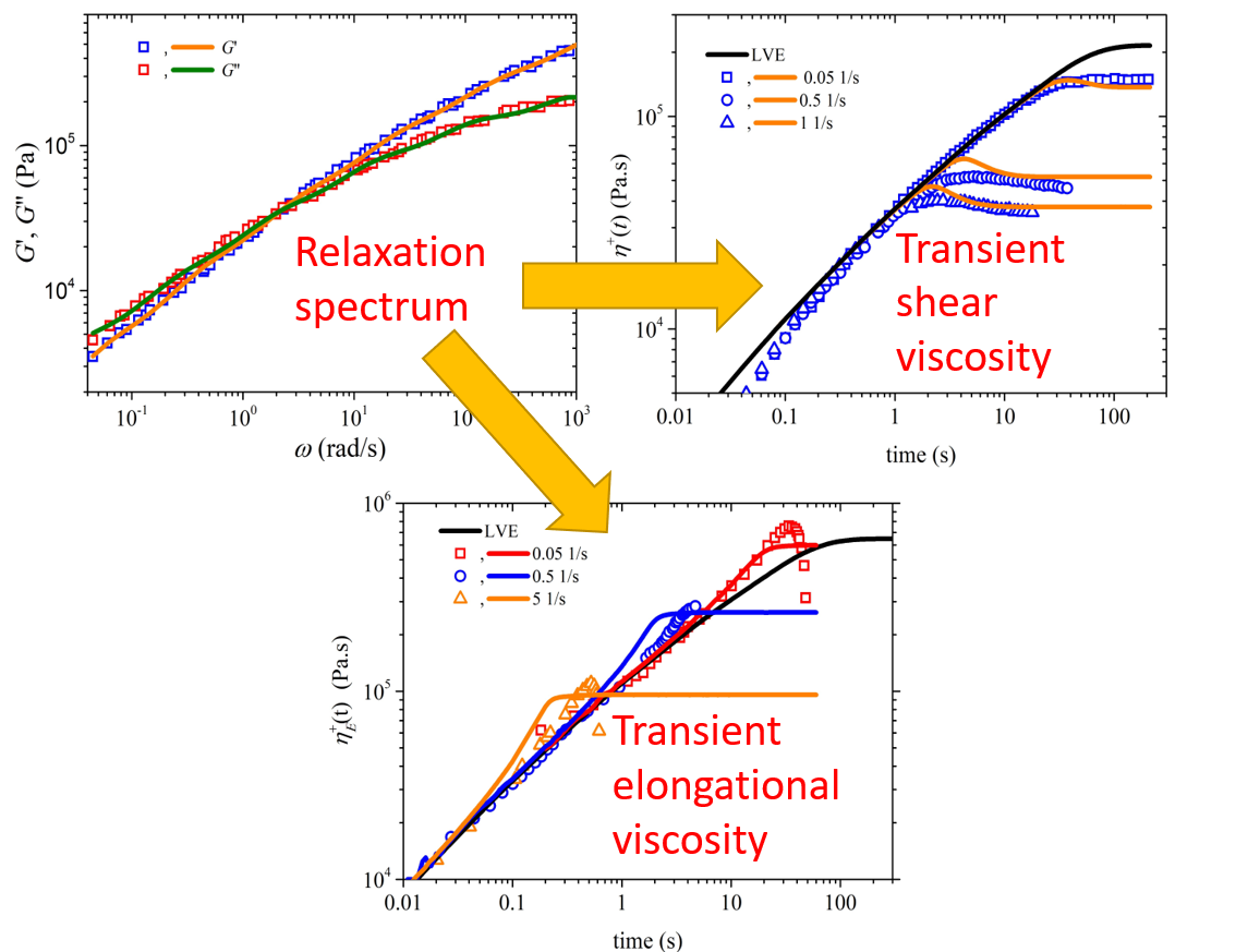
The FENE parameter can be easily calculated via b e = 3 ( 0.82 ) 2 M e / ( M 0 C ) as mentioned above. For PE M0=14 gr/mole, whereas C=7.3 and Me = 828 g/mole (see Table 3.3, p. 151 of Ref. [38]). These values yield be = 16.34. We will compare against the experimental data of Konaganti et al. [14] that have performed rheological measurements of the sample HDPE-1 reported by the same group [39] for which Mw=206 kg/mole; thus, the number of entanglements is equal to Z≈249. The relaxation spectrum is the same as the one used by Konaganti et al. [14] (see their Table 2 for T=200 oC) but is also provided in Table 1, and it was obtained by fitting the storage and loss moduli, Eqs. (7), with the corresponding experimental data. The comparison against the experimental storage and loss moduli is available in Figure 1.
All the remaining parameter values are obtained by fitting the model predictions against the experimental data; note that for simplicity we assume that each parameter has the same value for all modes although, in general, different values for each mode could be considered (e.g., see the work of Konaganti et al. [14]). The following values of the model parameter are chosen to provide a good comparison against the experimental data: ξ=0.02, α=0.3, βccr=4×10⁻⁴, and k=-3.5.

4.1. Comparison with start-up shear flow data

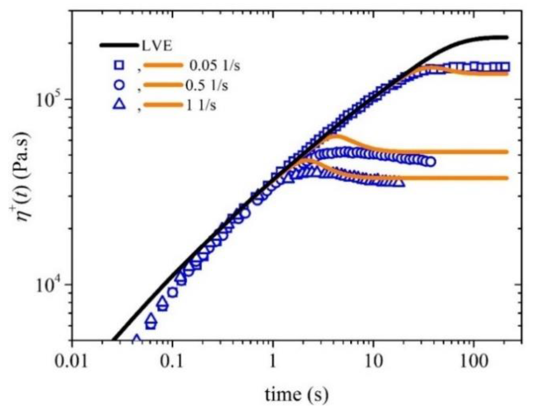
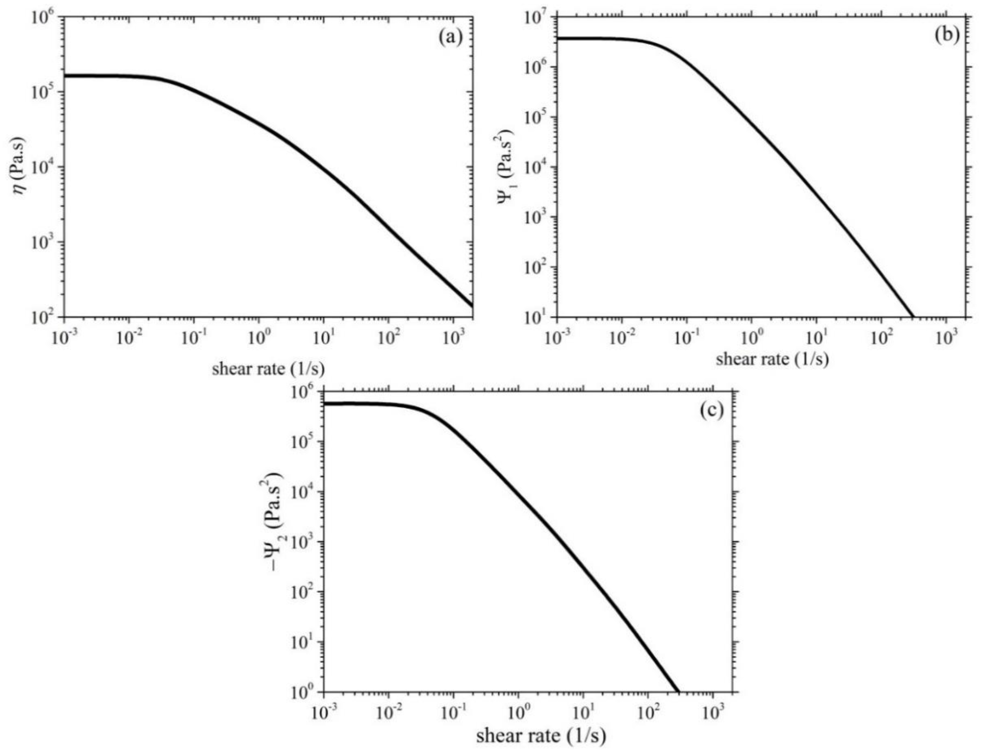
Figure 2 illustrates the comparison between the experimental data for the growth of the shear viscosity upon inception of shear flow and the simulated results obtained from the model. The experimental data (blue symbols) were collected at three different shear rates: 0.05 1/s, 0.5 1/s, and 1 1/s, whereas the orange lines represent the simulated shear viscosity values at the corresponding shear rates. It can be observed that the model accurately captures the trends and magnitude of the shear viscosity over time. Note that although a non-zero value of ξ is employed, the undershoots produced are too small to note in the scale used for Figure 2. Although no experimental data are provided, we further provide here the corresponding prediction of the growth of the first and second normal stress coefficients in Figure 3, and the steady-state values of all viscometric material functions in Figure 4.

4.2. Comparison with start-up uniaxial elongational flow data

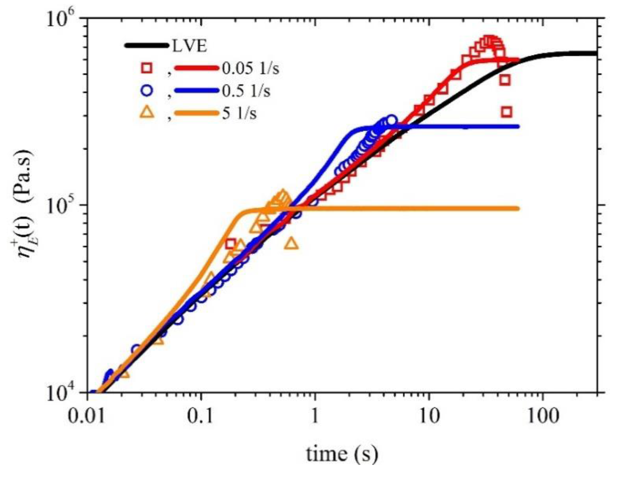
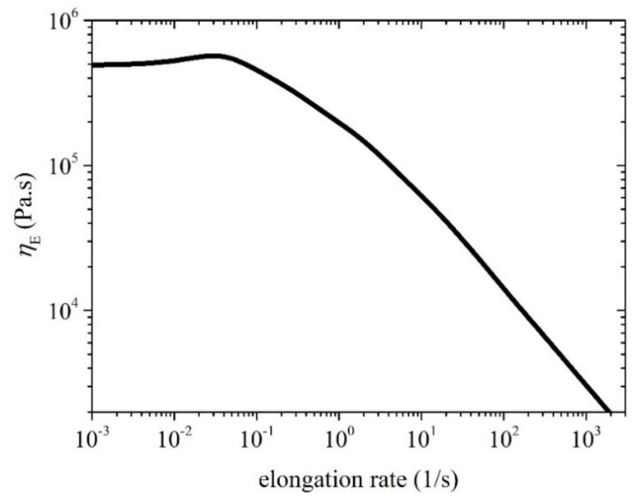
In Figure 5 we provide the comparison of the model predictions with the experimental measurements of Konaganti et al. [14] for the growth of the elongational viscosity as a function of time upon inception of uniaxial elongational at three different stretch rates: 0.05 1/s, 0.5 1/s, and 5 1/s. The comparison employs the same parameter values as the ones used in Figure 2 except ξ=0, as instructed by Stephanou et al. [35], and the corresponding steady-state prediction is provided in Figure 6. Given that the parameter values were selected based on the start-up shear data (Figure 2), the comparison is noted to be adequately well. Overall, the proposed model demonstrates good agreement with the experimental data, indicating its effectiveness in describing the rheological behavior of polymers of industrial significance.

5. Conclusions

In this work, we have developed the multiple-mode version of a generalized, conformation-tensor based viscoelastic model for polymer melts, that has been proposed recently by one of us [22], by making use of the generalized bracket formalism of Beris and Edwards [34]. As its forerunner, the monodisperse version [22], it accounts for the most significant effects that can be realized in entangled polymers systems: anisotropic drag, finite extensibility, non-affine motion (leading to the exhibition of a transient stress undershoot at large shear rates), and variable chain relaxation due to convective constraint release. The multiple-mode version of the model has been shown to bear a very good predictive capability with regards to the industrial experimental data for HDPE of Konaganti et al. [14].
The model in its present form considers only strictly linear chains. Industrial samples, particularly LDPE, are never strictly linear having either short or long branches distributed along their entire backbone. There is clear evidence that all material functions of PE are considerably affected by even the presence of low levels of long chain branching [40]. We therefore need to generalize it and allow for the explicit consideration of branches, following the guidelines provided by the pom-pom [26] and, its thermodynamically-admissible version, the Pom-pon [27] model. Furthermore, the multi-mode version does not explicitly consider the molecular weight (MW) distribution of industrial samples, such as the log-normal of gamma distributions that are able to describe experimental distributions [41]. As such, we should also generalize it to handle molecular weight distribution following the work of Schieber [42], [43]. This generalized constitutive model will allow for the more accurate prediction of the rheological response of polymeric systems used industrially that do possess an extensive spectrum of MW and not a very narrow distribution as it is customarily assumed when deriving a constitutive model. Only then would polymer engineers be able to accurately use the predictions of the revised constitutive model against the rheological response noted in actual industrial processes. Our findings provide a foundation for future research aimed at enhancing the properties of high MW polymers for diverse applications.

Author Contributions

Conceptualization, P.S.S.; Data curation, P.C.K. and P.S.S.; Formal analysis, P.C.K. and P.S.S.; Investigation, P.C.K. and P.S.S.; Methodology, P.S.S.; Project administration, P.S.S.; Resources, P.C.K. and P.S.S.; Software, P.C.K. and P.S.S.; Supervision, P.S.S.; Validation, P.C.K. and P.S.S.; Visualization, P.C.K. and P.S.S.; Writing – original draft, P.C.K.; Writing – review & editing, P.S.S.

Funding

This research received no funding

Institutional Review Board Statement

Not applicable

Informed Consent Statement

Not applicable

Data Availability Statement

Not applicable

Conflicts of Interest

The author declares no conflict of interest.

Notes

1

References

  1. Z. Tadmor and C. G. Gogos, Principles of Polymer Processing, 2nd Edition. 2006. [Online]. Available: https://books.google.ca/books?id=TUdmBk1_mlAC.
  2. Graham, M.D. The sharkskin instability of polymer melt flows. Chaos: Interdiscip. J. Nonlinear Sci. 1999, 9, 154–163, . [CrossRef]
  3. Barone, J.R.; Plucktaveesak, N.; Wang, S.Q. Interfacial molecular instability mechanism for sharkskin phenomenon in capillary extrusion of linear polyethylenes. J. Rheol. 1998, 42, 813–832, . [CrossRef]
  4. Baig, C.; Stephanou, P.S.; Tsolou, G.; Mavrantzas, V.G.; Kröger, M. Understanding Dynamics in Binary Mixtures of Entangled cis-1,4-Polybutadiene Melts at the Level of Primitive Path Segments by Mapping Atomistic Simulation Data onto the Tube Model. Macromolecules 2010, 43, 8239–8250, . [CrossRef]
  5. Stephanou, P.S.; Baig, C.; Tsolou, G.; Mavrantzas, V.G.; Kröger, M. Quantifying chain reptation in entangled polymer melts: Topological and dynamical mapping of atomistic simulation results onto the tube model. J. Chem. Phys. 2010, 132, 124904, . [CrossRef]
  6. Stephanou, P.S.; Baig, C.; Mavrantzas, V.G. Projection of atomistic simulation data for the dynamics of entangled polymers onto the tube theory: calculation of the segment survival probability function and comparison with modern tube models. Soft Matter 2011, 7, 380–395, . [CrossRef]
  7. Stephanou, P.S.; Baig, C.; Mavrantzas, V.G. Toward an Improved Description of Constraint Release and Contour Length Fluctuations in Tube Models for Entangled Polymer Melts Guided by Atomistic Simulations. Macromol. Theory Simulations 2011, 20, 752–768, . [CrossRef]
  8. Stephanou, P.S.; Mavrantzas, V.G. Accurate prediction of the linear viscoelastic properties of highly entangled mono and bidisperse polymer melts. J. Chem. Phys. 2014, 140, 214903, . [CrossRef]
  9. V. Nassehi, Practical Aspects of Finite Element Modelling of Polymer Processing. 2002.
  10. R. G. Larson, Constitutive Equations for Polymer Melts and Solutions, 1st ed. Butterworth-Heinemann, 1988.
  11. R. B. Bird, R. C. Armstrong, and O. Hassager, Dynamics of polymeric liquids. Volume 1. Fluid mechanics., 2nd Editio. Wiley-Interscience, 1987.
  12. J. D. Ferry, Viscoelastic properties of polymers, 1st ed. John Wiley & Sons, Ltd, 1980.
  13. X. -L Luo and R. I. Tanner, “Finite element simulation of long and short circular die extrusion experiments using integral models,” Int. J. Numer. Methods Eng., 25, 9–22, (1988),.
  14. Konaganti, V.K.; Ansari, M.; Mitsoulis, E.; Hatzikiriakos, S.G. Extrudate swell of a high-density polyethylene melt: II. Modeling using integral and differential constitutive equations. J. Non-Newtonian Fluid Mech. 2015, 225, 94–105, . [CrossRef]
  15. Langouche, F.; Debbaut, B. Rheological characterisation of a high-density polyethylene with a multi-mode differential viscoelastic model and numerical simulation of transient elongational recovery experiments. Rheol. Acta 1999, 38, 48–64, . [CrossRef]
  16. Shiromoto, S.; Masutani, Y.; Tsutsubuchi, M.; Togawa, Y.; Kajiwara, T. The effect of viscoelasticity on the extrusion drawing in film-casting process. Rheol. Acta 2010, 49, 757–767, . [CrossRef]
  17. Khan, S.A.; Larson, R.G. Comparison of Simple Constitutive Equations for Polymer Melts in Shear and Biaxial and Uniaxial Extensions. J. Rheol. 1987, 31, 207–234, . [CrossRef]
  18. M. (Masao) Doi and S. F. (Samuel F. Edwards, The theory of polymer dynamics, 1st ed. Clarendon Press, 1988. Accessed: May 17, 2023. [Online]. Available: https://global.oup.com/academic/product/the-theory-of-polymer-dynamics-9780198520337.
  19. Ianniruberto, G.; Marrucci, G. On compatibility of the Cox-Merz rule with the model of Doi and Edwards. J. Non-Newtonian Fluid Mech. 1996, 65, 241–246, . [CrossRef]
  20. Marrucci, G. Dynamics of entanglements: A nonlinear model consistent with the Cox-Merz rule. J. Non-Newtonian Fluid Mech. 1996, 62, 279–289, . [CrossRef]
  21. Baig, C.; Mavrantzas, V.G.; Kröger, M. Flow Effects on Melt Structure and Entanglement Network of Linear Polymers: Results from a Nonequilibrium Molecular Dynamics Simulation Study of a Polyethylene Melt in Steady Shear. Macromolecules 2010, 43, 6886–6902, . [CrossRef]
  22. Stephanou, P.S.; Tsimouri, I.C.; Mavrantzas, V.G. Simple, Accurate and User-Friendly Differential Constitutive Model for the Rheology of Entangled Polymer Melts and Solutions from Nonequilibrium Thermodynamics. Materials 2020, 13, 2867, . [CrossRef]
  23. Stephanou, P.S.; Schweizer, T.; Kröger, M. Communication: Appearance of undershoots in start-up shear: Experimental findings captured by tumbling-snake dynamics. J. Chem. Phys. 2017, 146, 161101, . [CrossRef]
  24. Costanzo, S.; Huang, Q.; Ianniruberto, G.; Marrucci, G.; Hassager, O.; Vlassopoulos, D. Shear and Extensional Rheology of Polystyrene Melts and Solutions with the Same Number of Entanglements. Macromolecules 2016, 49, 3925–3935, . [CrossRef]
  25. Stephanou, P.S.; Kröger, M. Non-constant link tension coefficient in the tumbling-snake model subjected to simple shear. J. Chem. Phys. 2017, 147, 174903, . [CrossRef]
  26. T. C. B. Mcleish, ; R G Larson, and R. G. Larson, “Molecular constitutive equations for a class of branched polymers: The pom-pom polymer,” J. Rheol., 42, 81–110, (1998),.
  27. Öttinger, H.C. Thermodynamic admissibility of the pompon model for branched polymers. Rheol. Acta 2001, 40, 317–321, . [CrossRef]
  28. Inkson, N.J.; McLeish, T.C.B.; Harlen, O.G.; Groves, D.J. Predicting low density polyethylene melt rheology in elongational and shear flows with “pom-pom” constitutive equations. J. Rheol. 1999, 43, 873–896, . [CrossRef]
  29. Soulages, J.; Schweizer, T.; Venerus, D.; Kröger, M.; Öttinger, H. Lubricated cross-slot flow of a low density polyethylene melt. J. Non-Newtonian Fluid Mech. 2008, 154, 52–64, . [CrossRef]
  30. W. M. H. Verbeeten, G. W. M. Peters, and F. P. T. Baaijens, “Differential constitutive equations for polymer melts: The extended Pom–Pom model,” J. Rheol., 45, 823–843, (2001),.
  31. Soulages, J.; Hütter, M.; Öttinger, H.C. Thermodynamic admissibility of the extended Pom-Pom model for branched polymers. J. Non-Newtonian Fluid Mech. 2006, 139, 209–213, . [CrossRef]
  32. Hoyle, D.M.; Harlen, O.G.; Auhl, D.; McLeish, T.C.B. Non-linear step strain of branched polymer melts. J. Rheol. 2009, 53, 917–942, . [CrossRef]
  33. Stephanou, P.S.; Tsimouri, I.C.; Mavrantzas, V.G. Flow-Induced Orientation and Stretching of Entangled Polymers in the Framework of Nonequilibrium Thermodynamics. Macromolecules 2016, 49, 3161–3173, . [CrossRef]
  34. A. N. Beris and B. J. Edwards, Thermodynamics of Flowing Systems: with Internal Microstructure. New York: Oxford University Press, 1994.
  35. Stephanou, P.S.; Baig, C.; Mavrantzas, V.G. A generalized differential constitutive equation for polymer melts based on principles of nonequilibrium thermodynamics. J. Rheol. 2009, 53, 309–337, . [CrossRef]
  36. Öttinger, H.C. Beyond Equilibrium Thermodynamics; Wiley: Hoboken, NJ, United States, 2005; ISBN: 9780471666585.
  37. Marrucci, G.; Ianniruberto, G. Flow-induced orientation and stretching of entangled polymers. Philos. Trans. R. Soc. A: Math. Phys. Eng. Sci. 2003, 361, 677–688, . [CrossRef]
  38. R. G. Larson, The Structure and Rheology of Complex Fluids. New York, United States: Oxford University Press, 1999.
  39. E. Behzadfar, M. Ansari, V. K. Konaganti, and S. G. Hatzikiriakos, “Extrudate swell of HDPE melts: I. Experimental,” J. Nonnewton. Fluid Mech., 225, 86–93, (2015),.
  40. Wood-Adams, P.M. The effect of long chain branches on the shear flow behavior of polyethylene. J. Rheol. 2001, 45, 203–210, . [CrossRef]
  41. Rogošić, M.; Mencer, H.; Gomzi, Z. Polydispersity index and molecular weight distributions of polymers. Eur. Polym. J. 1996, 32, 1337–1344, . [CrossRef]
  42. Schieber, J.D. Kinetic theory of polymer melts. VIII. Rheological properties of polydisperse mixtures. J. Chem. Phys. 1987, 87, 4917–4927, . [CrossRef]
  43. J. D. Schieber, “Kinetic theory of polymer melts. IX. Comparisons with experimental data,” The Journal of Chemical Physics, 87. 4928–4936, 1987.
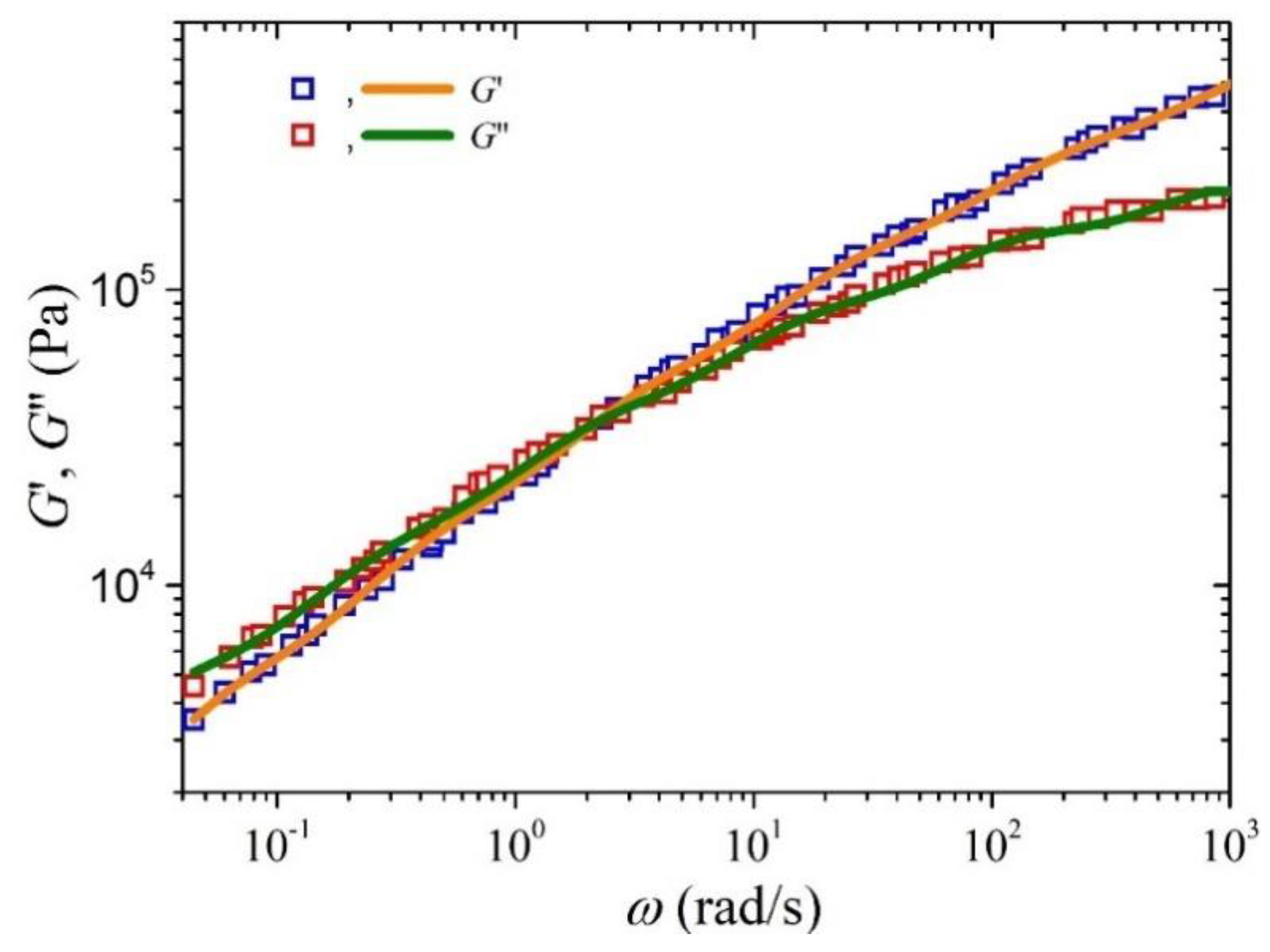
Figure 1. Comparison of the model predictions with the experimental data presented in Ref. [14] for the storage and loss moduli at 200 oC of an HDPE sample. The relaxation spectrum is provided in Table 1.
Preprints 79852 g001
Figure 2. Growth of the shear viscosity prediction (orange lines) upon inception of the shear flow at three different dimensionless shear rates and comparison with the experimental data (blue symbols) considered in Ref. [14] . The thick orange line depicts the LVE envelope, Equation (15a).
Preprints 79852 g002
Figure 3. Model predictions (red, blue and orange lines) of the growth of the first (a) and second (b) normal stress coefficients, upon inception of shear flow. The thick black lines depict the LVE envelope, Eqs. (15b) and (15c). Same parameter values as in Figure 2.
Preprints 79852 g003
Figure 4. Model predictions of the steady-state a) shear viscosity, (b) first, and (c) second normal stress coefficient of the HDPE-1 sample. Same parameter values as in Figure 2.
Preprints 79852 g004
Figure 5. Comparison of the model predictions (lines) with the experimental measurements (symbols) of Konaganti et al. [14] for the growth of the elongational viscosity as a function of time for several stretch rates. The thick black line depicts the LVE envelope, Equation (16). Same parameter values as in Figure 2 except ξ=0.
Preprints 79852 g005
Figure 6. Model predictions of the steady-state uniaxial elongational viscosity. Same parameter values as in Figure 2 except ξ=0.
Preprints 79852 g006
Table 1. Relaxation spectrum [14].
Mode G ˜ e ( i ) (Pa) τ CR ( i ) (s)
1 387,808 0.00086
2 185,307 0.0075
3 93,338 0.0548
4 37,766 0.403
5 12,934 2.99
6 5,025 30.78
Disclaimer/Publisher’s Note: The statements, opinions and data contained in all publications are solely those of the individual author(s) and contributor(s) and not of MDPI and/or the editor(s). MDPI and/or the editor(s) disclaim responsibility for any injury to people or property resulting from any ideas, methods, instructions or products referred to in the content.
Copyright: This open access article is published under a Creative Commons CC BY 4.0 license, which permit the free download, distribution, and reuse, provided that the author and preprint are cited in any reuse.
Prerpints.org logo

Preprints.org is a free preprint server supported by MDPI in Basel, Switzerland.

Subscribe

© 2024 MDPI (Basel, Switzerland) unless otherwise stated