1. Introduction
Pursuit problems are of critical importance in several engineering and science applications today, including navigation, warfare, and so on. The study of these problems were first motivated by the problems of navigating ships in the age of exploration [
1,
3]. The
Apollonius pursuit problem was defined as that of finding whether a ship leaving from a point
A with a constant velocity
will intercept another ship leaving from point
B with a constant velocity
The situation of adaptive pursuit, where the pursuer maneuvers their “ship” adaptively according to position of the pursuee, was first studied by Bouguer [
5], who derived the so-called “radiodrome” as the curve of best pursuit.
More recently, this problem has been generalized in various ways, for example, allowing for variable speeds of the pursuer and the pursued, adaptive strategies for the pursued, energy constraints on the pursuer and pursued, as well as errors in observation and imperfect information. For a detailed survey on these various generalizations and constraints, we refer the reader to [
2,
7,
10,
13] and references therein.
In this work, we look at a class of pursuit problems admitting a simple geometrical argument for establishing the locus and further generalize the result using analytic arguments. We demonstrate that certain popular challenge problems typically posed to senior high school or freshmen undergraduate students in physics admit simple solutions as special cases of these results.
2. Problem Setup and Main Results
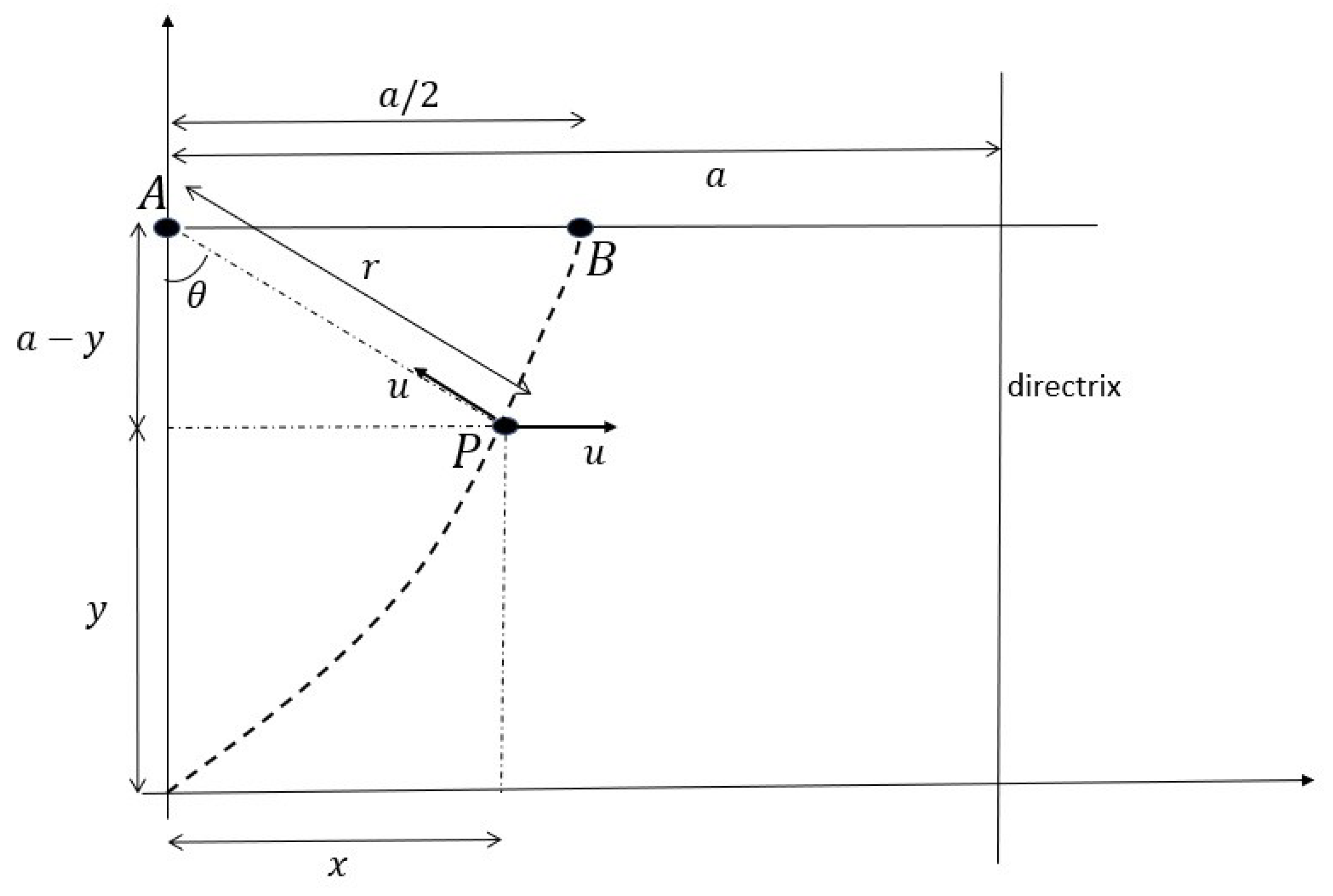
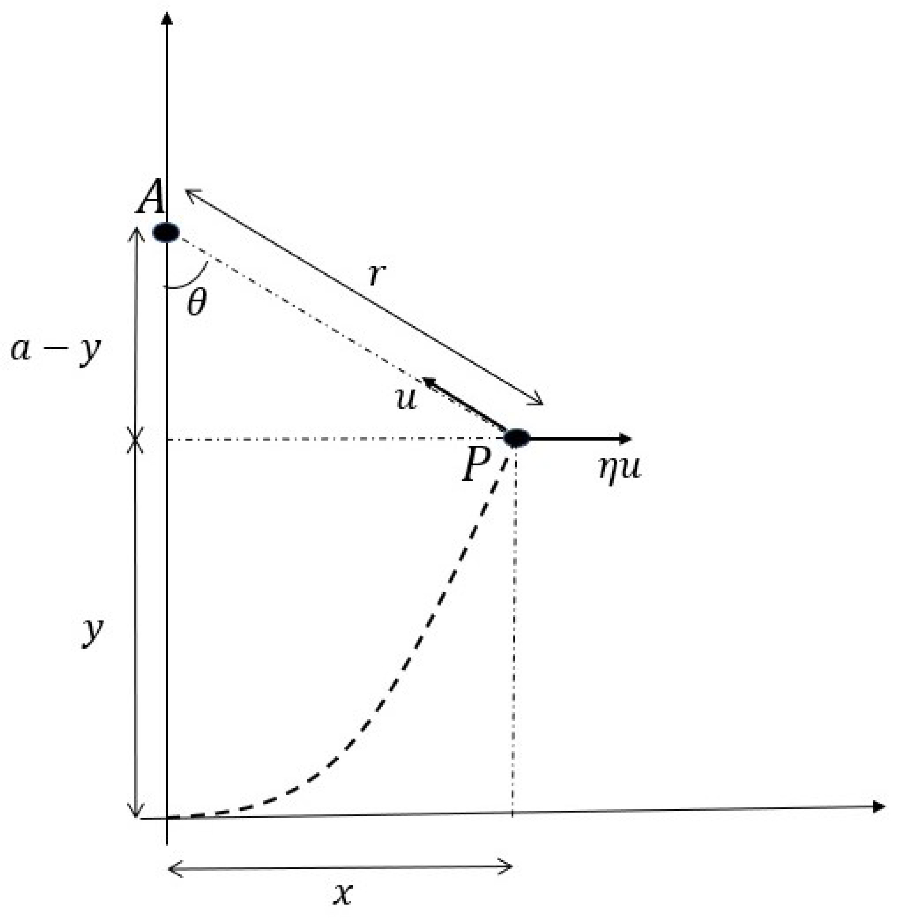
The main setup of our problem is illustrated in
Figure 1 and
Figure 2. A pursuer
P wishes to catch a stationary “prey”
A by always approaching
A with speed
pointing towards
while drifting in the
x direction with constant speed
The problem now is to find the trajectory of
P and decide if
P will ever be able to catch
The general solution to this problem for
in presented in Theorem 1 and requires an analytic treatment; however, for the special case
it can be argued geometrically that the trajectory is a conic section, without delving into any analytic derivation. The critical observation that makes this argument possible is that for this case (see
Figure 1), the component of the velocity of
P along the
x axis remains identical to the component of the velocity of
P in the instantaneous direction of
each being equal to
Therefore, the total amount of drift in the
x direction till any time
t is equal to the reduction in the distance between
P and
A till
This observation immediately enables us to prove the following lemma.
Lemma 1.
Suppose a point starting from the origin wishes to reach the point A by always trying to approach A at speed as shown in Figure 1. However, there is a constant “current” of the same speed u towards the positive x direction, which causes the path of P to drift. Then, the resultant locus of P is a parabola with focus at given by the equation
for
Geometric proof of Lemma 1. Consider a line parallel to the
y-axis, at a distance
a (i.e., the line satisfying
). By the previous arguments, the distance of the man from this line remains equal to his distance from
This leads us immediately to conclude, from elementary geometry, that the locus of the path is a parabola with focus at
A and directrix given by the line
Moreover, the final point
B lies on the perpendicular drawn from the focus to the directrix and is therefore the vertex. The length of the latus rectum is then given by
and the parabola “opens” in the negative
x direction with vertex at
The equation of the path is then given by
□
Finding the time dependence of the motion, however, requires some additional effort. To that end, note that since the positive
y component of the velocity is given by
we have
Setting
we then have
The integrated equation of motion is then given by
Integrating Equation
2 and re-arranging leads to
We now tackle the general case where the speed of the current is given by
for
As a first step, we present the following elementary result, which is a popular problem posed in elementary kinematics (see, for example, [
14] prob. 1.13, p. 13).
Lemma 2. For the pursuer reaches the point A, as depicted in Figure 2, at time
Proof. From
Figure 2, we have
and
Eliminating
between these relations leads to
Integrating this equation with the initial conditions
leads to
Setting
in (
4) leads to the result. □
Remark 1. We note that eqn (4) holds in general for any However, is finite only for
Remark 2.
We can use eqn (4) to provide a second proof of Lemma 1 as follows. Setting in (4) leads to
which yields eqn (1) on dividing both sides by
We now establish the most general result of this section.
Theorem 1.
The equation of path of the pursuer, with and θ as depicted in Figure 2, is given by
Further, the time dependence of the path is given by
The path equation (5) holds for for and for while (6) holds for for and for
Corollary 1.
We note here that Theorem 1 immediately recovers the result of Lemma 1 by setting In addition, setting in (6) (for ) leads to
which recovers the result of Lemma 2.
Proof of Theorem 1. We start from eqn (
4). Setting
in (
4) and solving for
r leads to
Now, going back to
Figure 2, we note that the
component of the velocity is given by
whence, we have
Eliminating
r between (
7) and (
8) lets us write down a linear differential equation in
and
as
The LHS of (
9) equals
while the RHS, with the substitution
can be written as
Here,
is obtained through a standard partial fraction decomposition (see, for example, [
18] Sec.
IV.5) and the constants
and
C are obtained as
Substituting (
12), (
13), (
14), and (
11) into (
10) leads to
Now, from
Figure 2, we have
and
Therefore, continuing (
15), we have
Now, using (
7) leads to
which simplifies to
Squaring (
16) and using
yields
Finally, solving for
x yields
which establishes the equation of the path. Using this equation of path in (
16) yields
Now, using (
7), we have, for
which simplifies to
establishing the time dependence for
Here,
follows by using
and
follows by substituting the expressions for
r and
x from (
18) and (
17), respectively. Note that the time dependence for the case
was already established in (
3). We demonstrate here an additional sanity check that seems to corroborate this result. We have, for
Setting recovers the time dependence expression for □
Remark 3.
Note that the analysis leading to (19) is merely asanity check
and not a rigorous proof, since we did not argue that t has to be continuous in η for each This can, however, be argued fairly easily from elementary results on ordinary differential equations; we point the interested reader to [16] and references therein.
3. Other Pursuit Problems
In this section, we briefly comment on a class of pursuit problems which are commonly stated in the following form. Referring again to
Figure 2, suppose the point
A moves horizontally with speed
and the pursuer
P always points their velocity vector towards
but there is no “current”. Clearly, the problem is equivalent to the setting in Theorem 1, but observed from a frame moving in the
x direction with velocity
Accordingly, for the scenario where
A moves in the positive
x direction, the
x coordinate of
P will be given by
according to the notation used in
Section 2, and
will remain unchanged. Thus, for this problem, we have, using (
5) and (
6),
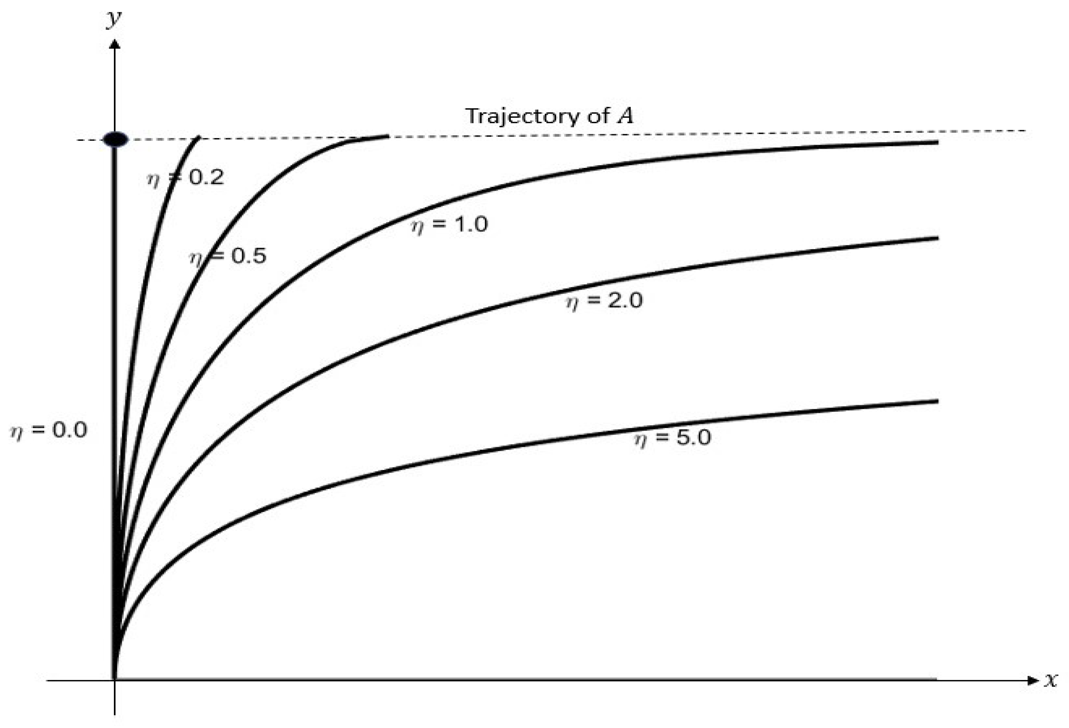
Figure 3 plots the pursuit trajectories (
20) for various values of
For
the trajectory approaches the trajectory of
A asymptotically, while for
the pursuer “catches” the prey at
Remark 4. This problem illustrates an interesting kinematic phenomenon: the trajectory in the first problem (Theorem 1) for is a finite segment of a parabola with no asymtotes, while the trajectory for the same problem observed from a different frame has an asymptote () and “looks” quite different (cf. Figure 3), even though the frames move with uniform velocity with respect to one another.
4. Discussions
The settings explored in this work can be generalized to include various scenarios, as allued to in the introduction. A geometric solution, while it may not be feasible in a general setting, might still provide a useful starting point and provide insights critical to solving many such problems. Bernhart [
20] and others [
7,
9,
23] have performed in-depth treatment specifically of the geometric properties and aspects of pursuit curves.
References
- E. Kasner and F. Supnick, “The Apollonian packing of circles”, Proceedings of the National Academy of Sciences USA 29(11), pp. 378–384, 1943.
- N. Ghaddar, S. Ganguly, L. Wang, and Y.-H. Kim, “A Lego-Brick Approach to Coding for Asymmetric Channels and Channels with State”, Proceedings of the International Symposium on Information Theory (ISIT), pp. 1367–1372, 2021.
- Isaac Weintraub, Eloy Garcia, and Meir E. Pachter, “Optimal guidance strategy for the defense of a non-manoeuverable target in 3-dimensions”, IET Control Theory & Applications 14(11), pp. 1531–1538, 2020.
- S. Ganguly and Y.-H. Kim, “Capacity Scaling for Cloud Radio Access Networks with Limited Orthogonal Fronthaul”, Proceedings of the International Symposium on Information Theory (ISIT), pp. 1472–1476, 2019.
- Pierre Bouguer, “Sur de nouvelles courbes auxquelles on peut donner le nom de lignes de poursuite”, Mémoires de mathématique et de physique tirés des registres de l’Académie royale des sciences, pp. 1–15, 1732.
- N. Ghaddar, S. Ganguly, L. Wang, and Y.-H. Kim, “A Lego-Brick Approach to Coding for Network Communication”, arXiv:2211.07208v3 [cs.IT], 2022.
- J. C. Barton and C. J. Eliezer, “On Pursuit Curves”, The Journal of the Australian Mathematical Society B41: Applied Mathematics (3), pp. 358–371, 2000.
- S. Ganguly and S. Pal, “Bounds on the Density of States and the Spectral Gap in CFT–2”, Phys. Rev. D 101(14):106022, pp. 1–4, May 2020.
- S. Ganguly, L. Wang, and Y.-H. Kim, “A Functional Construction of Codes for Multiple Access and Broadcast Channels”, Proceedings of the International Symposium on Information Theory (ISIT), pp. 1581–1586, 2020.
- C. Hoenselaers, “Chasing Relativistic Rabbits”, General Relativity and Gravitation (4), pp. 351–360, 1995.
- S. Ganguly and L. Wang, “Sliding-Window Gelfand–Pinsker Coding: General K-User Broadcast Channels”, Proceedings of the IEEE Information Theory Workshop (ITW), pp. 1–5, 2020.
- Richard P. Feynman, Robert B. Leighton, and Matthew Sands, The Feynman Lectures on Physics, Vol. 1 (Addison-Wesley, 1964), p. 3–10.
- S. Ganguly and Y.-H. Kim, “On the Capacity of Cloud Radio Access Networks”, Proceedings of the International Symposium on Information Theory (ISIT), pp. 2063–2067, 2017.
- I. E. Irodov, Problems in General Physics (Mir Publishers, 1988).
- S. Ganguly, S.-E. Hong, and Y.-H. Kim, “On the Capacity Regions of Cloud Radio Access Networks with Limited Orthogonal Fronthaul”, IEEE Trans. Inf. Theory 67(5), pp. 2958–2988, May 2021.
- Erwin Kreyszig, Advanced Engineering Mathematics (3rd ed.) (New York: Wiley, 1972).
- S. Ganguly, K. Sahasranand, and V. Sharma, “A New Algorithm for Distributed Nonparametric Sequential Detection”, Proceedings of the IEEE International Conference on Communications (ICC), pp. 1409–1415, 2014.
- Richard Courant, Differential and Integral Calculus, Vol. 1 (London: Blacktie & Son Limited, 1961).
- J. Ryu, S. Ganguly, Y.-H. Kim, Y.-K. Noh, and D. D. Lee, “Nearest Neighbor Density Functional Estimation based on Inverse Laplace Transform”, IEEE Trans. Inf. Theory 68(6), pp. 3511–3551, June 2022.
- Arthur Bernhart, “Curves of general pursuit”, Scripta Mathematica 24, 1959.
- S. Ganguly, K. Sahasranand, and V. Sharma, “A New Algorithm for Nonparametric Sequential Detection”, Proceedings of the National Conference on Communications (NCC), India, pp. 1–6, 2014.
- N. Ghaddar, S. Ganguly, L. Wang, and Y.-H. Kim, “A Lego-Brick Approach to Lossy Source Coding”, Proceedings of the 17th Canadian Workshop on Information Theory (CWIT), pp. 45–50, 2022.
- A. Guha and S. K. Biswas, “On Leonardo da Vinci’s cat and mouse problem”, Bulletin of the Institute of Mathematics and its Applications 30(1, 2), pp. 12–15, 1994.
|
Disclaimer/Publisher’s Note: The statements, opinions and data contained in all publications are solely those of the individual author(s) and contributor(s) and not of MDPI and/or the editor(s). MDPI and/or the editor(s) disclaim responsibility for any injury to people or property resulting from any ideas, methods, instructions or products referred to in the content. |
© 2023 by the authors. Licensee MDPI, Basel, Switzerland. This article is an open access article distributed under the terms and conditions of the Creative Commons Attribution (CC BY) license (http://creativecommons.org/licenses/by/4.0/).


