
Submitted:
18 July 2023
Posted:
19 July 2023
You are already at the latest version
Abstract
When implementing SVMs, two major problems are encountered: (a) the number of local minima increases exponentially with the number of samples and (b) the quantity of required computer storage, required for a regular quadratic programming solver, increases by an exponential mag-nitude as the problem size expands. The Kernel-Adatron family of algorithms gaining attention lately which has allowed it to handle very large classification and regression problems. Howev-er, these methods treat different types of samples (Noise, border, and core) in the same manner, which causes searches in unpromising areas and increases the number of iterations. In this work, we introduce a hybrid method to overcome these shortcomings, namely Optimal Recurrent Neu-ral Network Density Based Support Vector Machine (Opt-RNN-DBSVM). This method consists of four steps: (a) characterization of different samples, (b) elimination of samples with a low probability of being a support vector, (c) construction of an appropriate recurrent neural network based on an original energy function, and (d) solution of the system of differential equations, managing the dynamics of the RNN, using the Euler-Cauchy method involving an optimal time step. The RNN remembers the regions explored during the search process thanks to its recurrent architecture. We demonstrated that RNN-SVM converges to feasible support vectors and Opt-RNN-DBSVM has a very low time complexity compared to RNN-SVM with constant time step, and KAs-SVM. Several experiments were performed on academic data sets. We used several classification performances measures to compare Opt-RNN-DBSVM to different classification methods and the results obtained show the good performance of the proposed method.
Keywords:
Recurrent Neural Network(RNN)
; Support Vector Machine (SVM)
; Kernel-Adatron algorithm (KA)
; Euler-Cauchy Algorithm
MSC: 90C20; 90C29; 90C90; 93E20
1. Introduction
The classification problem is an NP-Hard problem that has many applications in medicine, industry, economics and other fields. Several types of classifiers have been proposed in the literature to solve this problem, including the approach called Support Vector Machine based on Quadratic Programming (QP) [5,6,7]. The difficulty in the implementation of SVMs on massive data comes in the fact that the quantity of required computer storage required for a regular QP solver increases by an exponential magnitude as the problem size expands.
In this paper, we introduce a new version of SVM that implements a preprocessing filter and a recurrent neural network, namely Optimal Recurrent Neural Network Density Based Support Vector Machine (Opt-RNN-DBSVM).
SVMs approaches are based on the existence of a linear separator which can be obtained by exploding the data in a higher dimensional space through appropriate kernel functions. Among all possible hyperplanes, the SVM searches for the one with the most confident separation margin for a good generalization. This issue takes the form of a nonlinear constrained optimization problem that is usually handled using optimization methods. Thanks to the Kuhen-Tuker conditions, all these methods pass to the dual versions and call the optimizations methods to find the support vectors on which the optimal margin is built. Unfortunately, the complexity in time and memory grow exponentially with the size of data sets; in addition, the number of local minima grows too, which influences the location of the separation margin and the quality of the predictions.
A primary area of research in the area of learning from empirical data through support vector machines (SVMs) and addressing classification and regression issues is the development of incremental learning designs when the size of the training dataset is massive \cite{SMOTE}.
Out of many possible candidates, avoiding the usage of regular Quadratic Programming (QP) solvers, the two learning methods gaining attention lately are Iterative Single-Data Algorithms (ISDA) and Sequential Minimal Optimization (SMO) [3,5,7,9]. ISDAs operate from a single sample at hand (pattern-based learning) towards the best fit solution. The Kernel AdaTron (KA) was the primary ISDA for SVMs, using kernel functions to mapping data to the high dimensional character space of SVMs P [2] and conducting AdaTron [1] processing in the character space. Platt’s SMO algorithm is an outlier among the so-called decomposition approaches introduced in [4,6], operating on a 2-samples workset of samples at a time. Because the decision for the two-point workset may be determined analytically, the SMO does not require the involvement of standard QP solvers. Due to it being analytically driven, the SMO has been especially wildly popular and is the most commonly utilized, analyzed, and further developed approach. Meanwhile, KA, though yielding somewhat comparable performance (accuracy and computational required time) in resolving classification issues, has not gained as much traction. The reason for this is twofold. First, up till lately [8], KA appeared to be restricted to classification tasks and second, it "missed" the flower of the robust theoretical framework. KA employs a gradient ascent procedure, and that fact also may have caused some researchers to be suspicious of the challenges posed by gradient ascent techniques in the presence of a perhaps ill-conditioned core array. In [10], for a lacking bias parameter b, the authors derive and demonstrate the equality of two apparently dissimilar ISDAs, namely a KA approach and an unbiased variant of the SMO training scheme [9] when constructing SVMs possessing positive definite kernels. The equivalence is applicable to the classification and regression tasks, and sheds additional insight in these apparently dissimilar methods of learning.
Despite the richness of the toolbox set up to solve the quadratic programs from SVM, and with the large amount of data generated by social networks, medical and agricultural fields, etc., the amount of computer memory required for a QP solver from the SVM dual grows hyper-exponentially and additional methods implementing different techniques and strategies are more than necessary.
Classical algorithms, namely ISDAs and SMO, do not distinguish between different types of samples (noise, border, and core) which causes searches in unpromising areas. In this work
we introduce a hybrid method to overcome these shortcoming, namely Optimal Recurrent Neural Network Density Based Support Vector Machine (Opt-RNN-DBSVM). This method proceeds in four steps: (a) characterization of different samples based on the density of the data sets (noise, core, and border), (b) elimination of samples with a low probability of being a support vector, namely core samples that are very far from the borders of different components of different classes, (c) construction of an appropriate recurrent neural network based on an original energy function making balance between the SVM-dual components (constraints and objective function) and insuring the feasibility of the network equilibrium points [3,4], and (d) solution of the system of differential equations, managing the dynamics of the RNN, using the Euler-Cauchy method involving an optimal time step. Due to its recurrent nature, the RNN was able to memorize locations visited during previous explorations. At one hand, two main interesting fundamental results were demonstrated: the convergence of RNN-SVM to feasible solutions and Opt-RNN-DBSVM has a very low time complexity compared to Const-RNN-SVM, SMO-SVM, ISDA-SVM, and L1QP-SVM.
On the other hand, several experimental studies were conducted based on well-known data sets. Based on well-known performance measures (Accuracy F1-score Precision Recal), Opt-RNN-DBSVM outperformed recurrent neural network-SVM with constant time step, Kernel-Adatron family of algorithms-SVM family, and well-known non-kernel models; In fact, Opt-RNN-DBSVM improved the accuracy, the F1Score, the precision, and the recall. Moreover, the proposed method requires a very small number of support vectors. The rest of this paper is organized as follows: In the second section, we give the flowchart of the proposed method. In the third section, we give the outline of our recent SVM versions called Density Based Support Vector Machine. The fourth section presents, in detail, the construction of recurrent neural networks associated with SVM-dual and the Euler-Cauchy algorithm that implements an optimal time step. In the fifth section, we give some experimental results. Finally, we give some conclusions and future extensions of Opt-RNN-DBSVM.
2. The architecture of the proposed method
The Kernel AdaTron (KA) algorithms, namely ISDAs, and SMO, treat different types of samples (noise, border, and core) in the same manner (all samples are considered for several iterations and supposed to be a support candidate with uniform probability), which causes searches in unpromising areas and increase the number of iterations. In this work, we introduce an economic method to overcome these shortcomings, namely Optimal Recurrent Neural Network Density Based Support Vector Machine (Opt-RNN-DBSVM). This method proceeds in four steps (see Figure 1): (1) Characterization of different samples based on the density of the data sets (noise, core, and border); to this end, two parameters are introduced: the size of the neighborhood of the current sample and the threshold that permits such categorization; (2) Elimination of samples with a low probability of being a support vector, namely core samples that are very far from the borders of different components of different classes and the noise samples that contain wrong information about the phenomenon under study. In our previews work [28], we demonstrate that such suppression does not influence the performance of the classifiers; (3) Construction of an appropriate recurrent neural network based on an original energy function making balance between the SVM-dual components (constraints and objective function) and ensuring the feasibility of the network equilibrium points [3,4]; (4) Solution of the system of differential equations, managing the dynamics of the RNN, using the Euler-Cauchy method involving an optimal time step. In this regard, the formula of the coming state of the neurons, of the constructed RNN, is introduced into the energy function, which leads to a 1-dimension quadratic optimization problem whose solution represents the optimal step of the Euler-Cauchy process that ensures a maximum decrease of the energy function [37]. The components of the produced equilibrium point represent the membership degrees of different samples to the support vectors data set.
3. Density based support vector machine
In the following, we denote by BD the set of N samples labeled, respectively, by , distributed via class . In our case, and ∈ {−1, +1}.
2.1. Classical support vector machine
The hyperplane we are looking for must satisfy the equation , where w is the weight that defines this SVM separator that satisfies the constraints family given by . To ensure a maximum margin, you need to maximize .
As the pattern are not linearly separable, we introduce the kernel functions K (that satisfy the Mercer conditions [9]) to explore the data in appropriate space. By introducing the Lagrange relaxation and writing the Kuhn-Tuker conditions, we obtain a quadratic optimization problem with a single linear constraint that we solve to determine the support vectors [18]. To address the problem of sutured constraints, some researchers have added the notion of a soft margin [8]. They employed N supplementary slack variables at every constraint . The sum of the relaxed variables is weighted and included in the cost function:
Here represents the transformation function derived from the function kernel K. We obtain the coming dual problem:
Several methods can be used to solve this optimization problem: gradient methods, linearization method Frank-Wolf method, generation column method, Newton method applied to the Kuhn system [23], sub-gradient methods, Dantzig algorithm, Uzawa algorithm [23], recursive neural networks [22], hill climbing, simulated annealing, search by calf, A*, genetic algorithm, ant colony [24], and particle swarm method [22] ... etc. Several versions of SVM were proposed in the literature among which we find the Least Squares Support Vector Machine Classifiers (LS-SVM) [12], the generalized support vector machines (G-SVM) [10], Fuzzy support vector machine [2,11], One class Support Vector Machine (OC-SVM) [13,18], Total Support Vector Machine (T-SVM) [14], Weighted Support Vector Machine (W-SVM) [15], Granular Support Vector Machines (G-SVM) [16], Smooth Support Vector Machine(S-SVM) [17], Proximity Support Vector Machine classifiers (P-SVM) [19], Multisurface proximal support vector machine classification via generalized eigenvalues (GEP-SVM) [20], and Twin support vector machines (T-SVM) [21] ... etc.
2.2. Density based support vector machine (DBSVM)
In this section, we give a short description of DBVSM method. We introduce real number r > 0 and the integer mp> 0, called min-points, and we define three types of samples: noise point, border point and interior point (or cord point). We showed that the interior points do not change their nature even when they are projected into another space by the kernel functions. Furthermore, we have established that such points cannot be selected as support vectors [28].
Definition 1.
Let . A point is said to be an Interior Point (or cord point) of S if there such that . The set of all interior point of S is denoted by
.
Definition 2.
For a given dataset BD, a non-negative real r and an integer mp, there exist three kind of samples.
- A simple is called if .
- A simple is called if and
- A simple is called if and there exists a such as .
Let K be a kernel function allowing to move from the space to the space using the transformation
Lemma 1.
[28] If a is a for a given and minpoints (mp), then is also a with appropriate ϵ′ and the same minpoints (mp).
Theorem 1.
[28] A cord point is either a noise-point or a Border-point.
Proposition 1.
[28] Lets be a real number. The cord point set, decreasing function for the inclusion operator.
Let be the set of the Lagrange multipliers where BM, CM, and N M are the Lagrange multipliers of the border samples, cord samples, and noise samples, respectively.
As the elements of and can not be selected to be support vectors, the reduced dual problem is given by:
In this work, as the (RD) problem is quadratic with linear constraint, we use the continuous Hopfield Network by proposing an original energy function in the coming section [26].
4. Recurrent neural network to optimal support vectors
The continuous Hopfield networks consist of interconnected neurons with a smooth sigmoid activation function (usually a hyperbolic tangent). The differential equation which governs the dynamics of the CHN is:
where and I are, respectively, the vectors of neuron states, the outputs, the weight matrix, and the biases. For a CHN of neurons, the state and output of the neuron i are relied on by the equation αi For an initial vector state , a vector is called an equilibrium point of the system 1, if and only if, such as . It should be noted if the energy function (or Lyapunov function) exists; the equilibrium point exists as well. Hopfield proved that the symmetry of the matrix of the weight is a sufficient condition for the existence of the Lyapunov function [25].
3.1. Continuous Hopfield network based on the original energy function
To solve the obtained dual problem via recurrent neural network [26], we propose the following energy function:
To determine the vector of the neurons biases, we calculate the partial derivatives of :
The components of the biases vector are given by:
To determine the connection weights between each neurons pair, we calculate the second partial derivatives of E:
The components of the weights matrix are given by:
To calculate the equilibrium point of the proposed recurrent neural network, we use the Euler-Cauchy iterative method:
- (1)
- Initialization: , and the step are randomly chosen;
- (2)
- Given and the step , the step is chosen such that is maximum and we calculate using: , then we calculate using the activation function , then the are given by: , where P is the projection operator on the set
- (3)
- Return to 1) until , where .
The Figure 2 shows the connection weights W between each pair of neurons.
Theorem 2.
If , else , where
Proof of Theorem 2.
We have and , then because
Thus
Finally, for , and for .
Concerning the constraint family satisfaction , we use the activation function.
, where is supposed to be a very large positive real number, which ensures .
We consider a kernel function such that .
Theorem 3.
A continuous Hopfield network has an equilibrium points if and .
Theorem 4.
If , then CHN-SVM has an equilibrium points.
Proof of Theorem 2.
We have then because K is symmetric. In the other hand
Then CHN-SVM has an equilibrium points
3.2. Continuous Hopfield network with optimal time step
In this section, we chose, mathematically, the optimal time size in each iteration of the Euler-Cauchy method to solve the dynamical equation of the recurrent neural network proposed in this paper.
At the end of the iteration, we know and let be the next step size permits to calculate using the formula: must be chosen such as at maximum.
As the activation function of the proposed neural network is the , then:
The matrix form of the energy function is:
where
At the iteration, the state is known, then is calculated by:
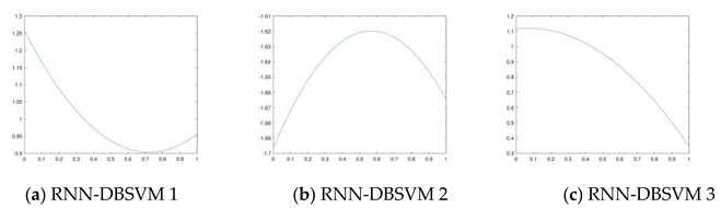
where is the actual time step that must be optimal. To this end, we substitute by in :
where
,
,
.
Thus the best time step is the minimum of . The Figure 3a–c gives different cases.
3.3. Opt-RNN-DBSVM algorithm
In this section, the procedures described in Section 2.2, 3.1, and 3.2 are summarized into Algorithm 1.
Algorithm 1. Opt-RNN-DBSVM.
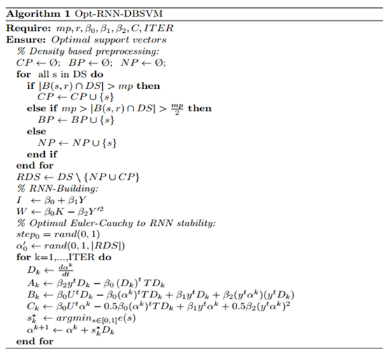
The input of Algorithm 1 is the radius r (the size of the neighborhood of the current sample), the minimum of samples mp into B(Current_sample, r) (that determines the type of this sample), the three lagrangian parameters (that makes a compromise between the dual components), the bound C of SVM [28], and the number of iterations (that represents an artificial convergence).
The Algorithm 1 processes in three macro-steps: Data preprocessing, RNN-SVM construction, and RNN-SVM equilibrium point estimation. The input of the first phase is the initial data set with labeled samples. Based on r and mp the algorithm determines the types of different samples based on the number of current sample neighbourhood discrete size. The output of this phase is a reduced sub-data set (The initial data set minus the core samples).
The Input of the second phase are the reduced data set, the Lagrangian parameters , and the SVM bound C. Based on the energy function built in 3.1 and on the first and second derivatives, the architecture of CHN-SVM is built; the bias and connection weights, which represent the output of this phase, are calculated. These later represent the input of the third phase and the Euler-Cauchy algorithm is used to calculate the degree of membership of different samples to the set of support vectors set; to ensure optimal decreasing of the energy function, at each iteration, an optimal step is determined by solving a quadratic 1-dimension optimization problem; see sub-section 3.2. At the convergence, the proposed algorithm produces the support vectors based on which Opt-RNN-DBSVM can predict the class of unseen samples.
Proposition 2.
If N, r, and ITER represent, respectively, the size of a labeled data set BD, the number of the remained samples(output of the preprocessing phase, and the number of iterations, then the complexity of algorithm 1 is
Proof of proposition 2.
First, in the preprocessing phase, we calculate, for each sample , the distance and we execute N comparisons to determine the type of each sample; thus the complexity of this phase is . Second, during ITER iterations, we update the activation of each neuron using the activation of all the other neurons to solve the reduced SVM-dual, thus the third phase has a complexity of
Finally, the complexity of algorithm 1 is Let’s denote Const- RNN-SVM the SVM version that implements recurrent neural network based on con- constant time step. Following the same reasoning, the complexity of Const-RNN-SVM is of
Notes: - As Kernel-Adatron Algorithm (KA) is the kernel version of SMO and ISDA and KA implements two embedded N-loops in each iteration, then the complexity of SMO and ISDA is of [40]. In addition, we consider L1QP-SVM that implements numerical linearalgebra Gauss–Seidel method [49], which implements two embedded N-loops in each iteration, then the complexity of SMO and ISDA is of . - For a very high size and high-density labeled data set, we have: thus and and .
Thus and , and
4. Experimentation
In this section, we compare Opt-RNN-DBSVM to several classifiers: Const-RNN-SVM (SVM based on a recurrent neural network using constant Euler-Cauchy time step), SMO- SVM, ISDA-SVM, L1QP-SVM, and some non-kernel classifiers (for example MLP, NB, KNN, Decision Tree...). The classifiers were tested on several data sets: iris, abalone, wine, ecoli, balance, liver, spect, seed, and PIMA (collected from the University of California at Irvine (UCI)[29]). The performance measures, used in this study, are accuracy, F1 score, precision, and recall.
4.1. Opt-RNN-DBSVM vs Const-CHN-SVM
In this section, we compare Opt-RNN-DBSVM to Const-RNN-SVM by considering different values of the Euler-Cauchy time step .
Table 1 and Table 2 give different values of accuracy, F1-score, precision, and recall on the considered data sets. The results show the superiority of Opt-RNN-DBSVM over Const-CHN-SVM; this superiority is quantified as follow:
where DATA is the set of different considering data sets. These results are not strange because Opt-RNN-SVM ensures an optimal decrease of the CHN energy function at each step.
4.2. Opt-RNN-DBSVM vs Classical-Optimizer-SVM
In this section, we give the performance of different Classical-Optimizer-SVM ( L1QP- SVM, ISDA-SVM, and SMO-SVM) applied to several datasets, and compare the number of support vectors obtained by the different Classical-Optimizer-SVM and Opti-RNN- SVM.
The Table 3 gives the values of the measures of accuracy, F1 score, precision, and recall of Classical-Optimizer-SVM on different datasets. The results show the superiority of Opt-RNN-DBSVM.
Figure 5, Figure 6, Figure 7 and Figure 8 illustrates, respectively, the support vectors obtained using L1QP-SVM, L1QP-SVM, SMO-SVM, and Opti-RNN-SVM applied to IRIS data. We note that (a) ISDA considers more than 96% as support vectors, which is really an exaggeration, (b) L1QP and SMO use a reasonable number of samples as support vectors, but most of them are duplicated, and (c) thanks to the preprocessing, Opt-RNN can reduce the number of support vectors by more than 32%, compared to SMO and L1QP, which allows it to overcome the over-learning phenomenon encountered with SMO and L1QP. Figure 8 gives the support vectors obtained by Opt-RNN-DBSVM applied to IRIS data.
4.3. Opt-RNN-DBSVM vs non-kernel classifiers
In this section, we compare Opt-RNN-DBSVM to several non-kernel classifiers, namely NiaveBayes [30], MLP [31], Knn [32], AdaBoostM1 [33], DecisionTree [34], SGDClassifier [35], Nearest Centroid Classifier [35], and Classical SVM [1].
Table 4 give the values of the measures accuracy, F1-score, precision, and recall for the considered data sets. The best performance is reached by Opt-RNN-DBSVM followed by classical methods SVM, Decision Tree, and Adabsot are close to the Opt-RNN-DBSVM method.
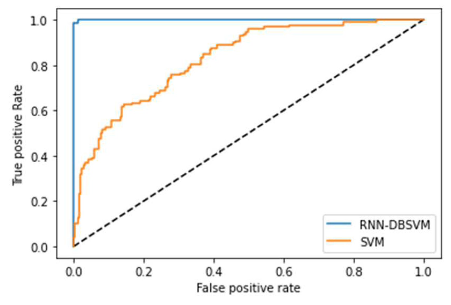
Additional comparison studies were performed on PIMA and Germandiabetes data sets and the ROC curves were used to calculate the AUC for the best performance obtained from each non-kernel classifier. Figure A6 and Figure A7 show the comparison of the ROC curves of the classifiers DT, KNN, MLP, NB, and Opt-RNN-DBSVM method, evaluated on the PIMA data set. We point out that Opt-RNN-DBSVM quickly converges to the best results and obtains more true positives for a small number of false positives compared to several classification methods. More comparisons are given in Appendix A; Figure A8 and Figure A9 show the comparison of the ROC curve of the classical SVM and Opt-RNN-DBSVM method, evaluated on the Germany diabetes data set.
5. Conclusions
The main challenges of SVM implementation are: the number of local minima and the amount of computer memory, required for solving the SVM-dual, increase exponentially with respect to the size of the data set. The Kernel-Adatron family of algorithms, ISDA and SMO, has handled very large classification and regression problems. However, these methods treat noise, boundary, and kernel samples in the same way, resulting in a blind search in unpromising areas. In this paper, we have introduced a hybrid approach to deal with these drawbacks, namely Optimal Recurrent Neural Network Density Based SupportVector Machine (Opt-RNN-DBSVM), which performs in four phases: Characterization of different samples, elimination of the samples having a weak probability to be support vector, building an appropriate recurrent neural network based on original energy function, and solving the differential equation system, governing the RNN dynamic, using Euler-Cauchy method implementing an optimal time step. Due to its recurrent nature, the RNN was able to memorize locations visited during previous explorations. On one hand, two main interesting fundamental results were demonstrated: the convergence of RNN-SVM to feasible solutions and Opt-RNN-DBSVM has a very low time complexity compared to Const-RNN-SVM, SMO-SVM, ISDA-SVM, and L1QP-SVM. On the other hand, several experimental studies were conducted based on well-known data sets (iris, abalone, wine, ecoli, balance, liver, spect, seed, pima). Based on credible performance measures (Accuracy F1-score Precision Recal), Opt-RNN-DBSVM outperformed Const-RNN-SVM, KAs- SVM, and some non-kernel models (cited Table 4). In fact, Opt-RNN-DBSVM improved accuracy by up to 3.43%, F1Score by up to 2.31%, precision by up to 7.52%, and recall by up to 6.5%. In addition, compared SMO-SVM, ISDA-SVM, and L1QP-SVM, Opt-RNN-DBSVM a reduction of the number of support vectors by up to 32%, which permits to save of memory for huge applications that implement several machine learning models. The main problem encountered in the implementation of Opt-RNN-DBSVM is the determination of the Lagrange parameters involved in the SVM energy function. In this sense, a genetic strategy will be introduced to determine these parameters considering each data set.
Funding
This research received no external funding.
Data Availability Statement
data are available under request.
Acknowledgments
This work was supported by Ministry of National Education, Professional Training, Higher Education and Scientific Research (MENFPESRS) and the Digital Development Agency (DDA) and CNRST of Morocco (Nos. Alkhawarizmi/2020/23).
Conflicts of Interest
The authors declare no conflict of interest.
Appendix A
Figure A1.
ABALONE data set.
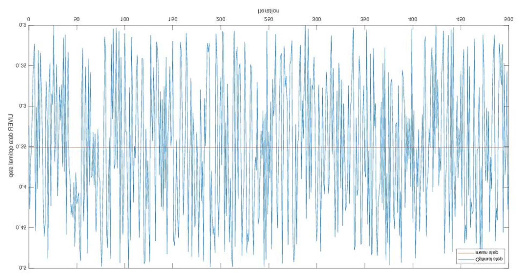
Figure A2.
PIMA data set.
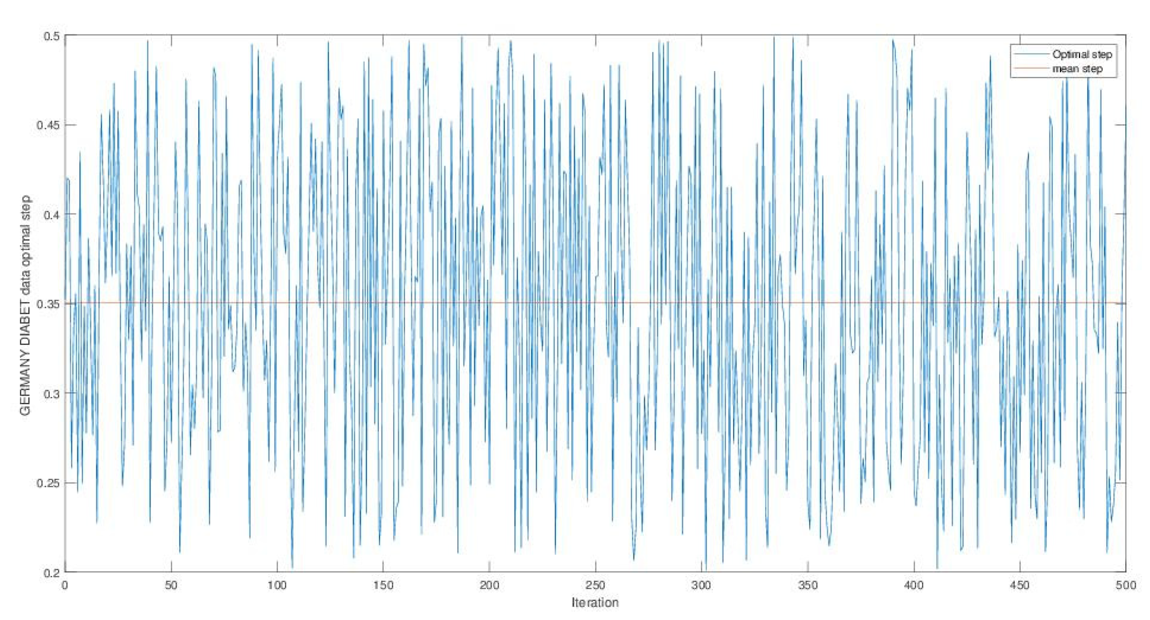
Figure A3.
WINE data set
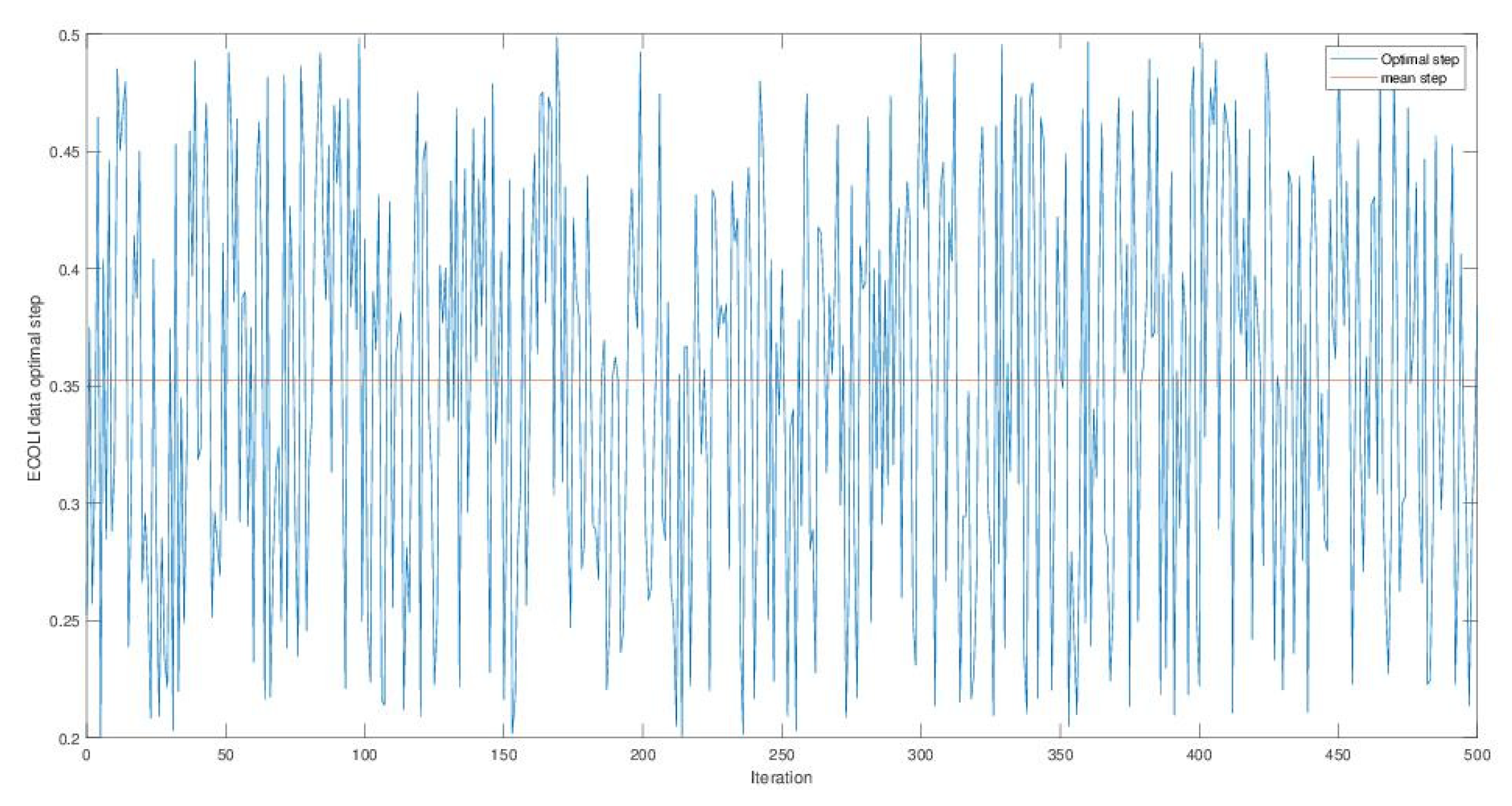
Figure A4.
SEED data set.
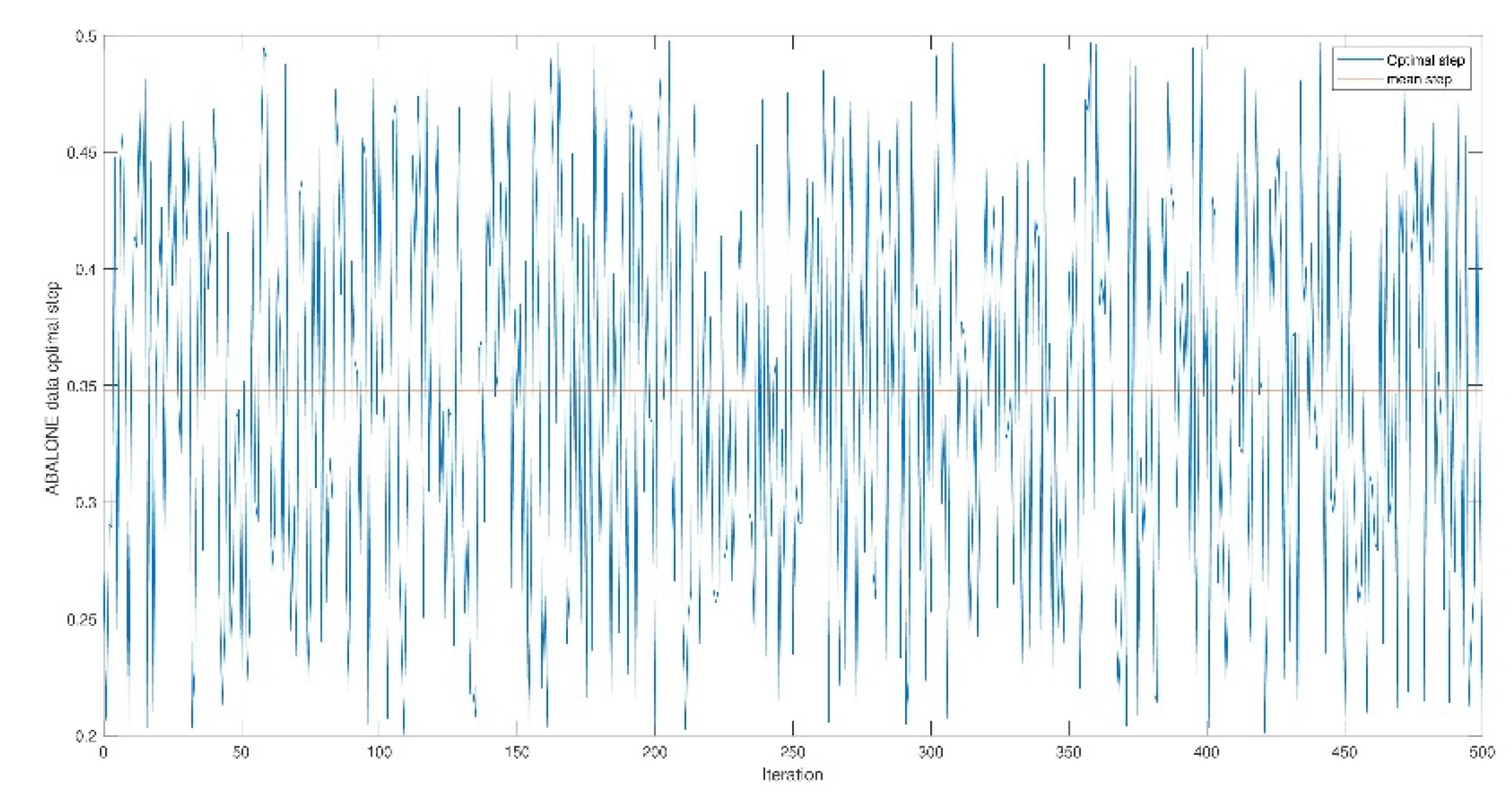
Figure A5.
GERMANY data set.
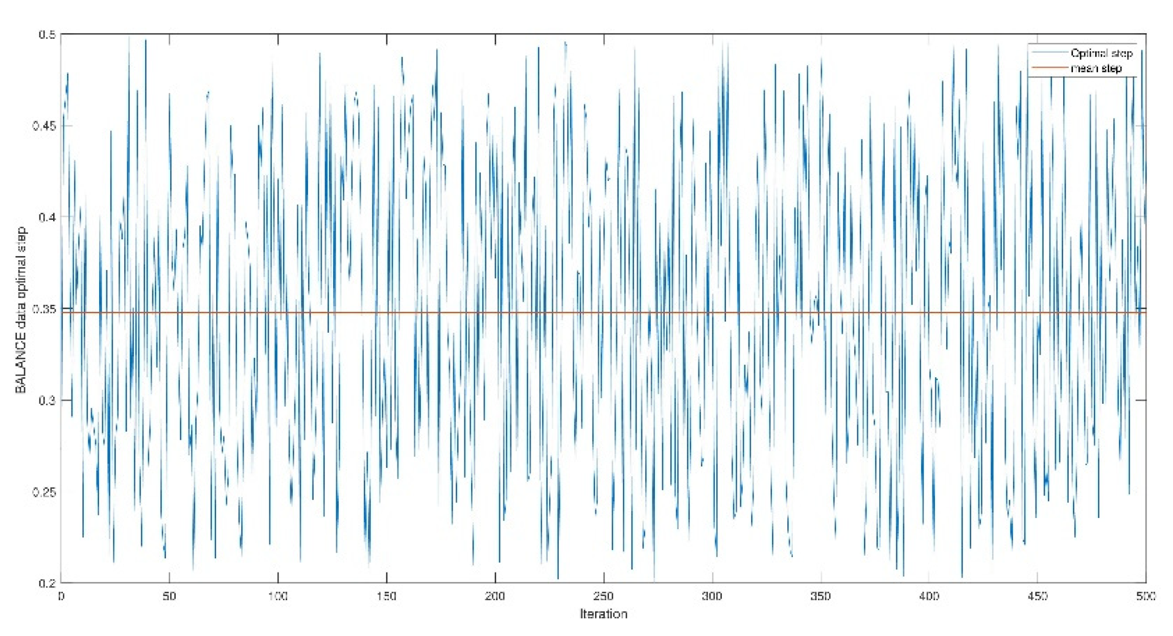
Figure A6.
RUC curve for the different classification methods applied to PIMA diabetes data set.
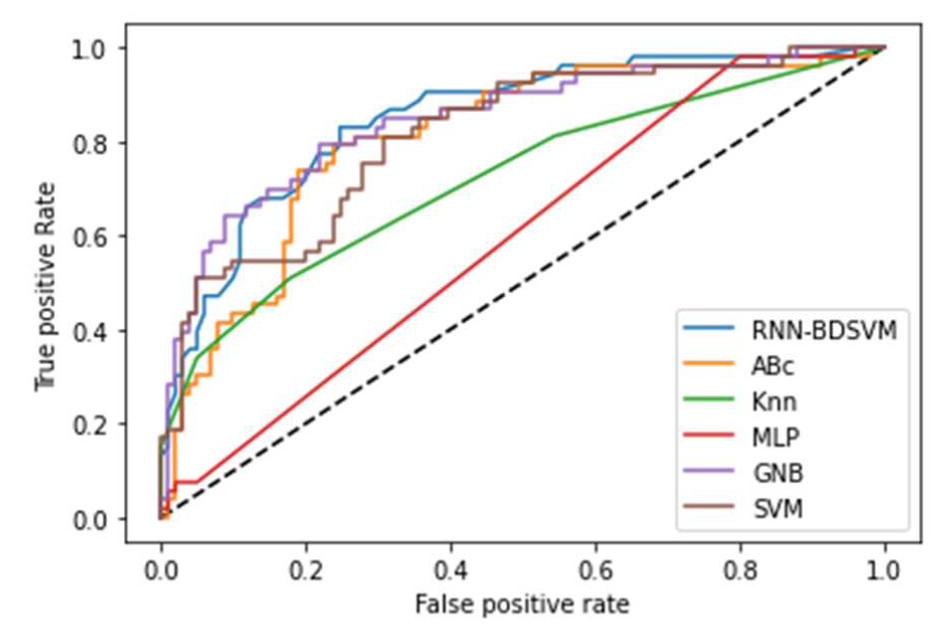
Figure A7.
Opt-RNN-DBSVM vs SVM RUC curve applied to PIMA diabetes data set.
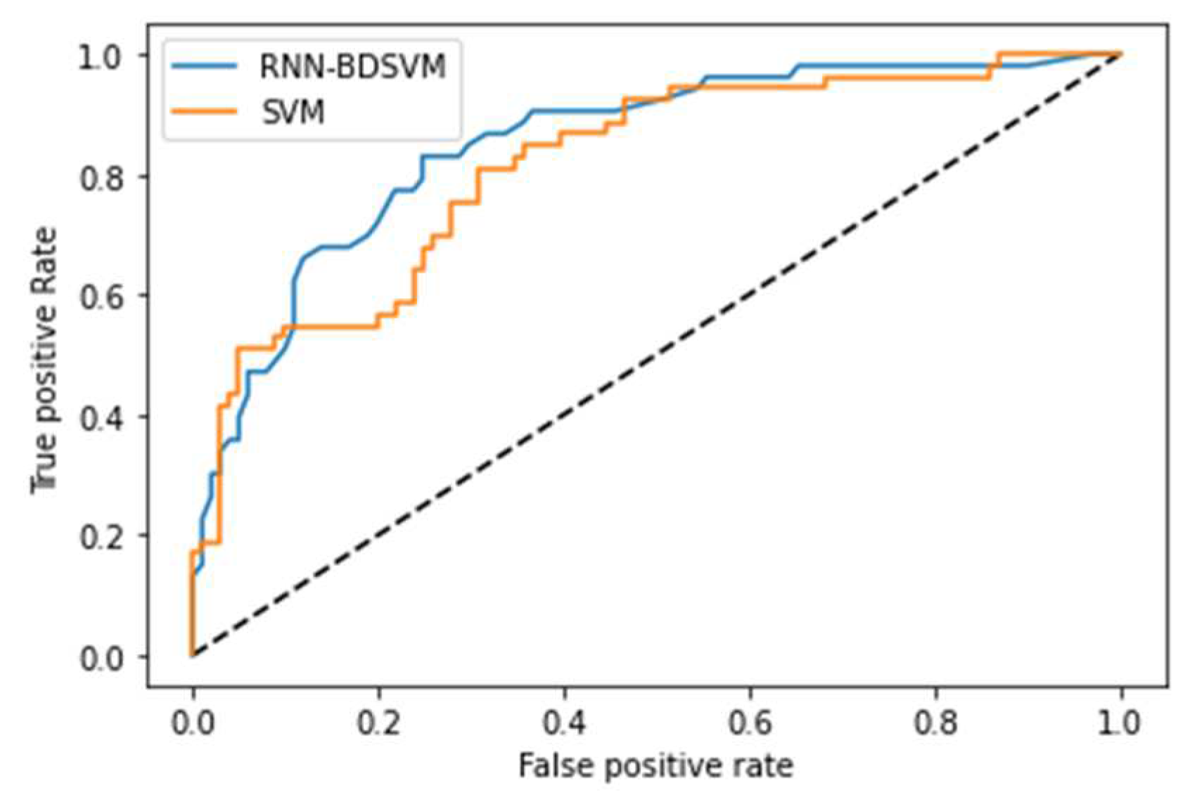
Figure A8.
RUC curve for the different classification methods applied to PIMA diabetes data set.
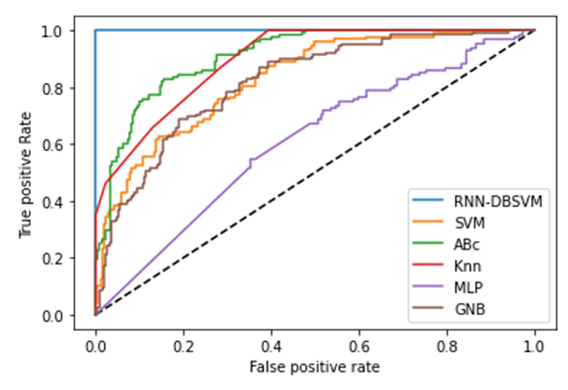
Figure A9.
Opt-RNN-DBSVM vs SVM RUC curve applied to PIMA diabetes data set.
References
- V. Vapnik, The Nature of Statistical Learning Theory. Springer Science and Business Media (1999).
- Schölkopf, B.; Smola, A.J.; Williamson, R.C.; Bartlett, P.L. New Support Vector Algorithms. Neural Comput. 2000, 12, 1207–1245, . [CrossRef]
- J.J. Hopfield, D.W. Tank, Neural computation of decisions in optimization problems. Biol. Cybern. 52 (1985) 1–25.
- K. Haddouch, & K. El Moutaouakil, New Starting Point of the Continuous Hopfield Network. In Int. Conf. on Big Data, Cloud Appl. Springer, Cham (2018, April) 379-389.
- W. Steyerberg, Clinical prediction models, Cham: Springer International Publishing (2019) 309-328.
- M. Law. How to build valid and credible simulation models. In 2019 Winter Simulation Conference (WSC) IEEE. (2019, December) 1402-1414.
- E. L. Glaeser, S. D. Kominers, M. Luca, & N. Naik. Big data and big cities: The promises and limitations of improved measures of urban life. Eco. Inqui. 56(1) (2018) 114-137.
- Cortes, V. Vapnik, Support-vector networks. Machine learning, 20(3) (1995) 273-297.
- J. Mercer, Functions of positive and negative type, and their connection the theory of integral equations. Philosophical transactions of the royal society of London. Ser. A, Cont. Pap. Math. Phy. Char., 209(441-458) (1909) 415-446.
- Ahmadi, M.; Khashei, M. Generalized support vector machines (GSVMs) model for real-world time series forecasting. Soft Comput. 2021, 25, 14139–14154, . [CrossRef]
- F. Lin, S. D.Wang, Fuzzy support vector machines. IEEE Trans. Neur. Netw. 13(2) (2002) 464-471.
- Aghbashlo, M.; Peng, W.; Tabatabaei, M.; Kalogirou, S.A.; Soltanian, S.; Hosseinzadeh-Bandbafha, H.; Mahian, O.; Lam, S.S. Machine learning technology in biodiesel research: A review. Prog. Energy Combust. Sci. 2021, 85, 100904, . [CrossRef]
- Schölkopf, B.; Platt, J.C.; Shawe-Taylor, J.; Smola, A.J.; Williamson, R.C. Estimating the Support of a High-Dimensional Distribution. Neural Comput. 2001, 13, 1443–1471, . [CrossRef]
- Bi, T. Zhang, Support vector classification with input data uncertainty. In Adv. Neur. Inf. Proc. syst. (2005) 161-168.
- Hazarika, B.B.; Gupta, D. Density-weighted support vector machines for binary class imbalance learning. Neural Comput. Appl. 2020, 33, 4243–4261, . [CrossRef]
- Guo, H.; Wang, W. Granular support vector machine: a review. Artif. Intell. Rev. 2019, 51, 19–32, . [CrossRef]
- Lee, Y.-J.; Mangasarian, O. SSVM: A Smooth Support Vector Machine for Classification. Comput. Optim. Appl. 2001, 20, 5–22, . [CrossRef]
- B. Schölkopf, AJ. Smola , F. Bach, Learning with kernels: support vector machines, regularization, optimization, and beyond. MIT press (2002).
- Xie, X.; Xiong, Y. Generalized multi-view learning based on generalized eigenvalues proximal support vector machines. Expert Syst. Appl. 2022, 194, 116491, . [CrossRef]
- Tanveer, M.; Rajani, T.; Rastogi, R.; Shao, Y.H.; Ganaie, M.A. Comprehensive review on twin support vector machines. Ann. Oper. Res. 2022, 1–46, . [CrossRef]
- Laxmi, S.; Gupta, S. Multi-category intuitionistic fuzzy twin support vector machines with an application to plant leaf recognition. Eng. Appl. Artif. Intell. 2022, 110, 104687, . [CrossRef]
- Ettaouil, M.; Elmoutaouakil, K.; Ghanou, Y. The Placement of Electronic Circuits Problem: A Neural Network Approach. Math. Model. Nat. Phenom. 2010, 5, 109–115, . [CrossRef]
- M. Minoux, Mathematical programming: theories and algorithms, Duond (1983).
- S. Russell and P. Norvig, Artificial Intelligence A Modern Approach, 3rd edition, by Pearson Education (2010).
- Hopfield, J.J. Neurons with graded response have collective computational properties like those of two-state neurons. Proc. Natl. Acad. Sci. USA 1984, 81, 3088–3092, doi:10.1073/pnas.81.10.3088.
- K. El Moutaouakil M. Ettaouil, Reduction of the continuous Hopfield architecture, J. Compu. Volume 4, Issue 8 (2012) pp. 64-70.
- K. El Moutaouakil, A. El Ouissari, A. Touhafi and N. Aharrane, "An Improved Density Based Support Vector Machine (DBSVM)," 5th Inter. Confe. Cloud Compu. Artif. Intel.: Techn. Appl. (CloudTech) (2020) pp. 1-7.
- El Ouissari, A.; El Moutaouakil, K. Density based fuzzy support vector machine: application to diabetes dataset. Math. Model. Comput. 2021, 8, 747–760, . [CrossRef]
- Dua, D. and Graff, C. UCI Machine Learning Repository [http://archive.ics.uci.edu/ml]. Irvine, CA: University of California, School of Information and Computer Science (2019).
- Wickramasinghe, I.; Kalutarage, H. Naive Bayes: applications, variations and vulnerabilities: a review of literature with code snippets for implementation. Soft Comput. 2021, 25, 2277–2293, . [CrossRef]
- O. Tolstikhin, N. Houlsby, A. Kolesnikov, L. Beyer, X. Zhai, T. Unterthiner, &A.Dosovitskiy, Mlp-mixer: An all-mlp architecture for vision. Adv. Neur. Inf. Proc. Sys. 34 (2021).
- Shokrzade, A.; Ramezani, M.; Tab, F.A.; Mohammad, M.A. A novel extreme learning machine based kNN classification method for dealing with big data. Expert Syst. Appl. 2021, 183, 115293, . [CrossRef]
- Chen, P.; Pan, C. Diabetes classification model based on boosting algorithms. BMC Bioinform. 2018, 19, 109, doi:10.1186/s12859-018-2090-9.
- Charbuty, B.; Abdulazeez, A. Classification Based on Decision Tree Algorithm for Machine Learning. J. Appl. Sci. Technol. Trends 2021, 2, 20–28, . [CrossRef]
- Almustafa, K.M. Classification of epileptic seizure dataset using different machine learning algorithms. Informatics Med. Unlocked 2020, 21, 100444, . [CrossRef]
- K E. Moutaouakil, & A. Touhafi, A New Recurrent Neural Network Fuzzy Mean Square Clustering Method. In 2020 5th International Conference on Cloud Computing and Artificial Intelligence: Technologies and Applications (CloudTech) IEEE (2020) 1-5.
- El Moutaouakil, K.; Yahyaouy, A.; Chellak, S.; Baizri, H. An Optimized Gradient Dynamic-Neuro-Weighted-Fuzzy Clustering Method: Application in the Nutrition Field. Int. J. Fuzzy Syst. 2022, 24, 3731–3744, . [CrossRef]
- El Moutaouakil, K.; Roudani, M.; El Ouissari, A. Optimal Entropy Genetic Fuzzy-C-Means SMOTE (OEGFCM-SMOTE). Knowledge-Based Syst. 2023, 262, . [CrossRef]
- Anlauf, J.K.; Biehl, M. The AdaTron: An Adaptive Perceptron Algorithm. EPL (Europhysics Lett. 1989, 10, 687–692, . [CrossRef]
- T.-T. Frieß, , Cristianini, N., Campbell, I. C. G., The Kernel-Adatron: a Fast and Simple Learning Procedure for Support Vector Machines. In Shavlik, J., editor, Proceedings of the 15th International Conference on Machine Learning, Morgan Kaufmann, San Francisco, CA (1998) 188–196.
- T.-M. Huang, V. Kecman, Bias Term b in SVMs Again, Proc. of ESANN 2004, 12th European Symposium on Artificial Neural Networks Bruges, Belgium, 2004.
- T. Joachims, Making large-scale svm learning practical. advances in kernel methods-support vector learning. http://svmlight. joachims.org/ (1999).
- V. Kecman, M. Vogt, T.-M. Huang, On the Equality of Kernel AdaTron and Sequential Minimal Optimization in Classification and Regression Tasks and Alike Algorithms for Kernel Machines, Proc. of the 11 th European Symposium on Artificial Neural Networks, ESANN, , Bruges, Belgium (2003) 215–222.
- E. Osuna, R. Freund, F. Girosi, An Improved Training Algorithm for Support Vector Machines. In Neural Networks for Signal Processing VII, Proceedings of the 1997 Signal Processing Society Workshop, (1997) 276–285.
- J. Platt, Sequential Minimal Optimization: A Fast Algorithm for Training Support Vector Machines, Microsoft Research Technical Report MSR-TR-98-14, (1998).
- Veropoulos, K., Machine Learning Approaches to Medical Decision Making, PhD Thesis, The University of Bristol, Bristol, UK (2001).
- M. Vogt, SMO Algorithms for Support Vector Machines without Bias, Institute Report, Institute of Automatic Control, TU Darmstadt, Darmstadt, Germany, (Available at http://www.iat.tu-darmstadt.de/vogt) (2002).
- V. Kecman, T. M.Huang, & M. Vogt, Iterative single data algorithm for training kernel machines from huge data sets: Theory andperformance. Support vector machines: Theory and Applications, (2005) 255-274.
- V. Kecman, Iterative k data algorithm for solving both the least squares SVM and the system of linear equations. In SoutheastCon IEEE (2015) 1-6.
Figure 1.
Opt RNN DBSVM Flowchart.
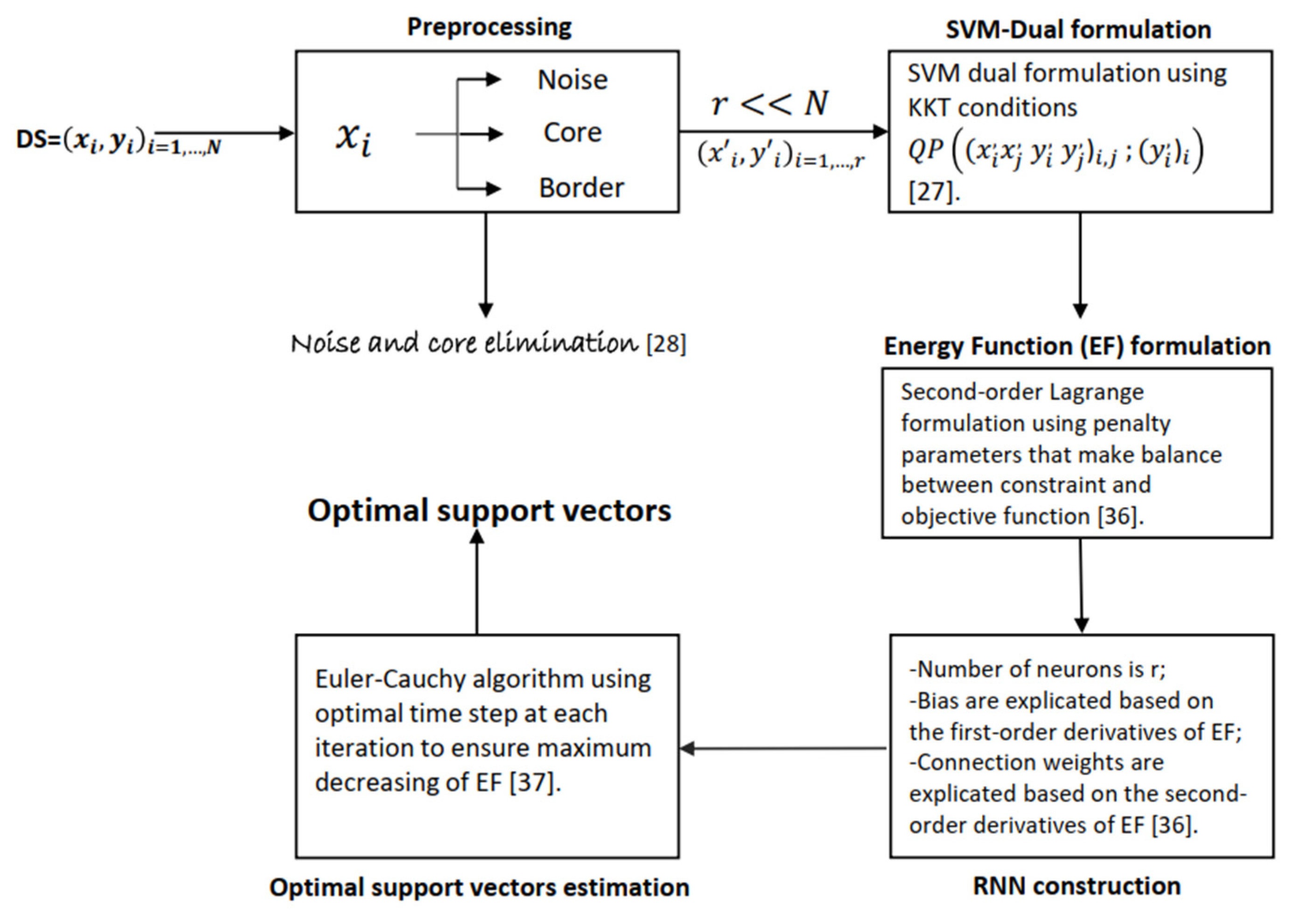
Figure 4.
IRIS data set.
Figure 5.
Vectors support obtained by ISDA algorithm.
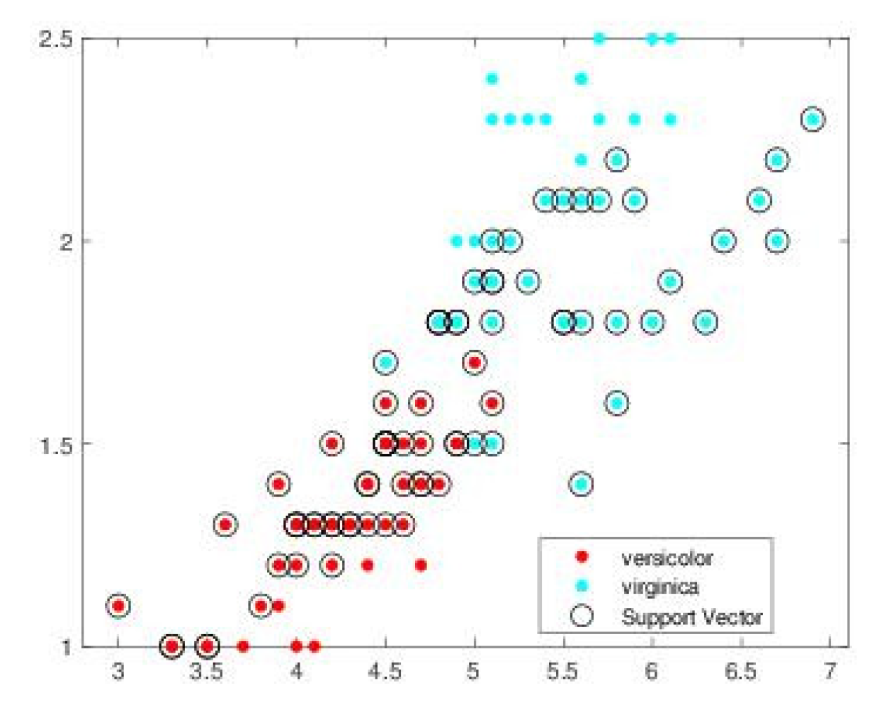
Figure 6.
Vectors support obtained by L1QP algorithm.
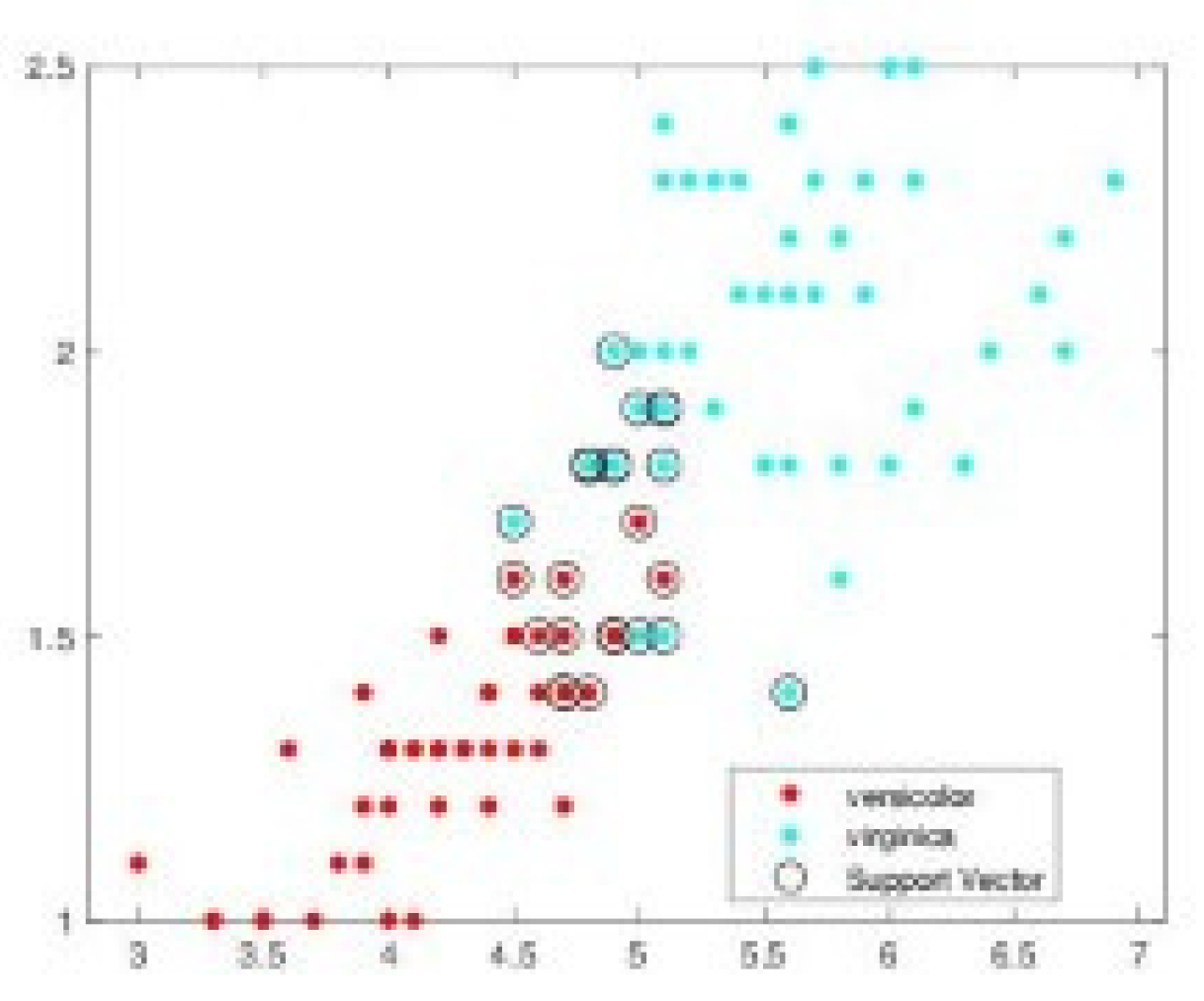
Figure 7.
Vectors support obtained by SMO algorithm.
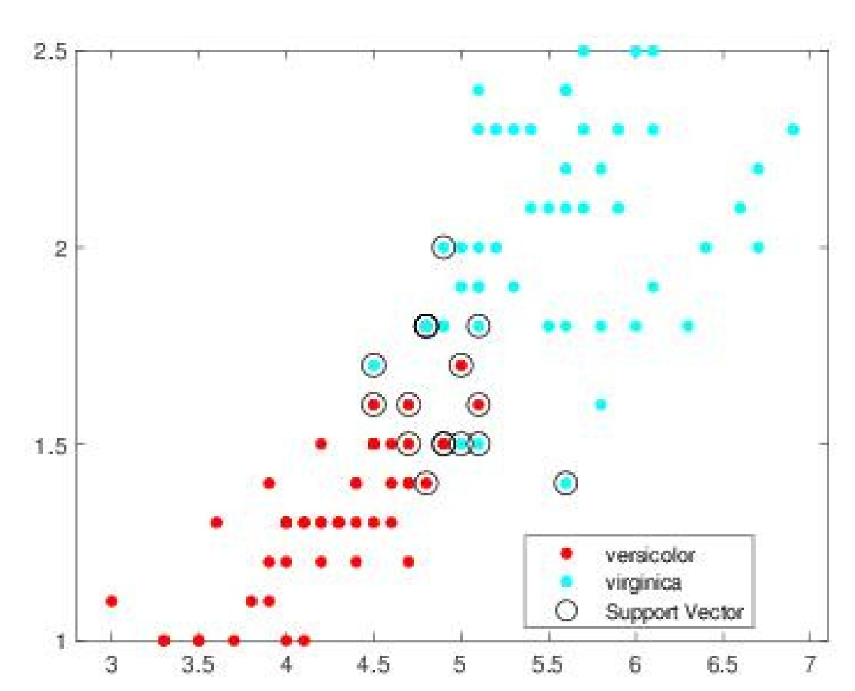
Figure 8.
Vectors support obtained by Opt RNN SVM algorithm.
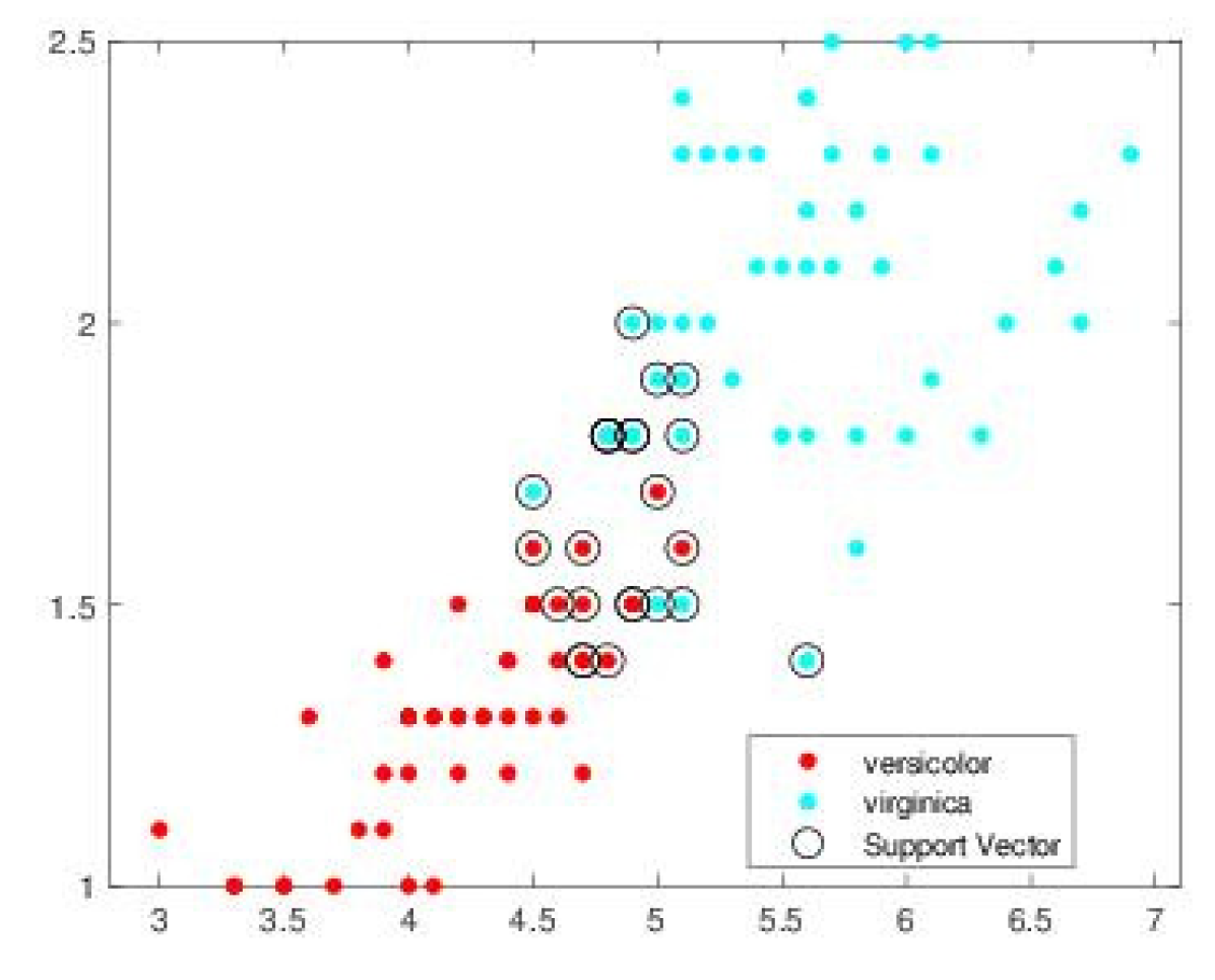

Table 1.
Performance of Const-CHN-SVM on different data sets for different values of time step.
| SVM-CHN s = .1 | SVM-CHN s = .2 | |||||||
|---|---|---|---|---|---|---|---|---|
| Accuracy | F1-score | Precision | Recall | Accuracy | F1-score | Precision | Recall | |
| Iris | 95.98 | 96.66 | 90.52 | 92.00 | 96.66 | 95.98 | 91.62 | 92.00 |
| Abalone | 80.98 | 40.38 | 82.00 | 27.65 | 80.66 | 40.38 | 81.98 | 27.65 |
| Wine | 79.49 | 78.26 | 73.52 | 74.97 | 79.49 | 78.26 | 73.52 | 74.97 |
| Ecoli | 88.05 | 96.77 | 97.83 | 97.33 | 88.05 | 97.77 | 97.83 | 97.99 |
| Balance | 79.70 | 70.7 | 55.60 | 62.70 | 79.70 | 70.7 | 55.60 | 62.70 |
| Liver | 80.40 | 77.67 | 77.90 | 70.08 | 80.40 | 77.67 | 77.90 | 70.08 |
| Spect | 92.12 | 90.86 | 91.33 | 90.00 | 97.36 | 99.60 | 97.77 | 1.00 |
| Seed | 85.71 | 83.43 | 92.70 | 75.04 | 85.71 | 83.43 | 92.70 | 75.04 |
| PIMA | 79.22 | 61.90 | 84.7 | 49.6 | 79.22 | 61.90 | 83.97 | 49.6 |
Table 2.
Performance of Const-CHN-SVM on different data sets for different values of time step.
| SVM-CHN s = .3 | SVM-CHN s = .4 | ||||||||||
| Accuracy | F1-score | Precision | Recall | Accuracy | F1-score | Precision | Recall | ||||
| Iris | 94.53 | 95.86 | 89.66 | 98.23 | 95.96 | 93.88 | 89.33 | 95.32 | |||
| Abalone | 77.99 | 51.68 | 83.85 | 30.88 | 81.98 | 41.66 | 83.56 | 33.33 | |||
| Wine | 80.23 | 77.66 | 74.89 | 74.97 | 81.33 | 77.65 | 73.11 | 74.43 | |||
| Ecoli | 88.86 | 95.65 | 96.88 | 97.33 | 86.77 | 97.66 | 97.83 | 97.95 | |||
| Balance | 79.75 | 70.89 | 55.96 | 62.32 | 79.66 | 70.45 | 56.1 | 66.23 | |||
| Liver | 80.51 | 78.33 | 77.9 | 70.56 | 80.40 | 77.67 | 77.90 | 70.08 | |||
| Spect | 97.63 | 98.99 | 97.81 | 98.56 | 96.40 | 98.71 | 96.83 | 97.79 | |||
| Seed | 85.71 | 83.43 | 92.70 | 75.88 | 85.71 | 83.43 | 92.70 | 75.61 | |||
| PIMA | 79.22 | 61.93 | 84.82 | 49.86 | 79.22 | 61.90 | 84.98 | 49.89 | |||
| SVM-CHN s = .5 | SVM-CHN s = .6 | ||||||||||
| Accuracy | F1-score | Precision | Recall | Accuracy | F1-score | Precision | Recall | ||||
| Iris | 94.53 | 95.86 | 89.66 | 98.23 | 95.96 | 93.88 | 89.33 | 95.32 | |||
| Abalone | 78.06 | 51.83 | 83.96 | 40.45 | 82.1 | 42.15 | 83.88 | 38.26 | |||
| Wine | 80.84 | 78.26 | 74.91 | 75.20 | 81.39 | 77.86 | 73.66 | 74.47 | |||
| Ecoli | 88.97 | 95.7 | 96.91 | 97.43 | 86.77 | 97.66 | 97.83 | 97.95 | |||
| Balance | 79.89 | 71.00 | 56.11 | 62.72 | 79.71 | 70.64 | 56.33 | 66.44 | |||
| Liver | 80.66 | 78.33 | 77.9 | 70.56 | 80.40 | 77.67 | 77.90 | 70.08 | |||
| Spect | 91.36 | 92.60 | 91.77 | 84.33 | 91.36 | 92.60 | 91.77 | 84.33 | |||
| Seed | 84.67 | 82.96 | 92.23 | 74.18 | 84.11 | 83.08 | 92.63 | 75.48 | |||
| PIMA | 79.12 | 61.75 | 84.62 | 49.86 | 79.12 | 61.33 | 84.68 | 48.55 | |||
| SVM-CHN s = .7 | SVM-CHN s = .8 | ||||||||||
| Accuracy | F1-score | Precision | Recall | Accuracy | F1-score | Precision | Recall | ||||
| Iris | 94.53 | 95.86 | 89.66 | 98.23 | 95.96 | 93.88 | 89.33 | 95.32 | |||
| Abalone | 77.99 | 51.68 | 83.85 | 30.88 | 81.98 | 41.66 | 83.56 | 33.33 | |||
| Wine | 80.23 | 77.66 | 74.89 | 74.97 | 81.33 | 77.65 | 73.11 | 74.43 | |||
| Ecoli | 88.86 | 95.65 | 96.88 | 97.33 | 86.77 | 97.66 | 97.83 | 97.95 | |||
| Balance | 79.75 | 70.89 | 55.96 | 62.32 | 79.66 | 70.45 | 56.1 | 66.23 | |||
| Liver | 80.51 | 78.33 | 77.9 | 70.56 | 80.40 | 77.67 | 77.90 | 70.08 | |||
| Spect | 94.36 | 84.60 | 83.77 | 85.99 | 94.36 | 84.60 | 83.77 | 85.99 | |||
| Seed | 85.71 | 83.43 | 92.70 | 75.88 | 85.71 | 83.43 | 92.70 | 75.61 | |||
| PIMA | 79.22 | 61.93 | 84.82 | 49.86 | 79.22 | 61.90 | 84.98 | 49.89 | |||
| SVM-CHN s = .9 | DBSVM optimal value of s | ||||||||||
| Accuracy | F1-score | Precision | Recall | Accuracy | F1-score | Precision | Recall | ||||
| Iris | 95.96 | 93.88 | 89.33 | 95.32 | 97.96 | 96.19 | 95.85 | 98.5 | |||
| Abalone | 81.98 | 41.66 | 83.56 | 33.33 | 98.38 | 96.07 | 96.18 | 93.19 | |||
| Wine | 81.33 | 77.65 | 73.11 | 74.43 | 96.47 | 95.96 | 96.08 | 96.02 | |||
| Ecoli | 86.77 | 88.46 | 90.77 | 91.19 | 91.82 | 97.66 | 97.83 | 97.95 | |||
| Balance | 79.66 | 70.45 | 56.1 | 66.23 | 91.31 | 90.33 | 89.54 | 90.89 | |||
| Liver | 80.40 | 77.67 | 77.90 | 70.08 | 88.10 | 85.95 | 86.00 | 85.50 | |||
| Spect | 94.36 | 84.60 | 83.77 | 85.99 | 95.55 | 86.20 | 85.28 | 86.31 | |||
| Seed | 85.71 | 83.43 | 86.18 | 75.61 | 88.90 | 84.31 | 92.70 | 84.40 | |||
| PIMA | 79.22 | 61.90 | 75.90 | 49.89 | 79.87 | 68.04 | 84.98 | 62.05 | |||
Table 3.
Performance of Classical-Optimizer-SVM on different data sets.
| L1QP-SVM | ISDA-SVM | |||||||
|---|---|---|---|---|---|---|---|---|
| Accuracy | F1-score | Precision | Recall | Accuracy | F1-score | Precision | Recal | |
| Iris | 71.59 | 62.02 | 70.80 | 55.17 | 82.00 | 83.64 | 76.67 | 92.00 |
| Abalone | 74.15 | 70.80 | 71.48 | 59.30 | 83.70 | 68.22 | 70.00 | 80.66 |
| Wine | 72.90 | 65.79 | 75.53 | 60.11 | 66.08 | 65.80 | 66.00 | 70.02 |
| Ecoli | 66.15 | 55.89 | 61.33 | 41.30 | 51.60 | 48.30 | 33.33 | 51.39 |
| Balance | 65.20 | 53.01 | 60.51 | 41.22 | 50.44 | 58.36 | 68.32 | 60.20 |
| Liver | 64.66 | 52.06 | 60.77 | 40.44 | 50.00 | 48.00 | 62.31 | 51.22 |
| Spect | 70.66 | 62.02 | 67.48 | 50.11 | 77.60 | 71.20 | 75.33 | 70.11 |
| Seed | 70.51 | 58.98 | 67.30 | 45.30 | 80.66 | 81.25 | 79.80 | 79.30 |
| PIMA | 65.18 | 53.23 | 60.88 | 39.48 | 49.32 | 44.33 | 48.90 | 50.27 |
| SMO- | SVM | CHN- | DBSVM optimal value of s | |||||
| Accuracy | F1-score | Precision | Recall | Accuracy | F1-score | Precision | Recal | |
| Iris | 71.59 | 62.02 | 70.80 | 55.17 | 97.96 | 96.19 | 95.85 | 98.5 |
| Abalone | 74.15 | 70.80 | 71.48 | 59.30 | 98.38 | 96.07 | 96.18 | 93.19 |
| Wine | 72.90 | 65.79 | 75.53 | 60.11 | 96.47 | 95.96 | 96.08 | 96.02 |
| Ecoli | 66.15 | 55.89 | 61.33 | 41.30 | 91.82 | 88.46 | 90.77 | 91.19 |
| Balance | 65.20 | 53.01 | 60.51 | 41.22 | 91.31 | 90.33 | 89.54 | 90.89 |
| Liver | 64.66 | 52.06 | 60.77 | 40.44 | 88.10 | 85.95 | 86.00 | 85.50 |
| Spect | 70.66 | 62.02 | 67.48 | 50.11 | 95.55 | 86.20 | 85.28 | 86.31 |
| Seed | 70.51 | 58.98 | 67.30 | 45.30 | 88.90 | 84.31 | 86.18 | 84.40 |
| PIMA | 65.18 | 53.23 | 60.88 | 39.48 | 79.87 | 68.04 | 75.90 | 62.05 |
Table 4.
Comparison between Opt-RNN-DBSVM and different classification methods on the Iris and abalone data sets.
Table 4.
Comparison between Opt-RNN-DBSVM and different classification methods on the Iris and abalone data sets.
| Iris | ||||
| Method | Accuracy | F1-score | Precision | Recall |
| Niave Bayes | 90.00 | 87.99 | 77.66 | 1.00 |
| MLP | 26.66 | 0.00 | 0.00 | 0.00 |
| Knn | 96.66 | 95.98 | 91.62 | 1.00 |
| AdaBoostM1 | 86.66 | 83.66 | 71.77 | 1.00 |
| Dicision Tree | 69.25 | 76.12 | 70.01 | 69.55 |
| SGDClassifier | 76.66 | 46.80 | 1.00 | 30.10 |
| Random Forest Classifier | 90.00 | 87.99 | 77.66 | 1.00 |
| Nearest Centroid Classifier | 96.66 | 95.98 | 91.62 | 1.00 |
| Classical SVM | 96.66 | 95.98 | 91.62 | 1.00 |
| Opt-RNN-DBSVM | 97.96 | 92.19 | 95.85 | 96.05 |
| Abalone | ||||
| Method | Accuracy | F1-score | Precision | Recall |
| Niave Bayes | 68.89 | 51.19 | 41.37 | 67.33 |
| MLP | 62.91 | 47.63 | 36.32 | 47.63 |
| Knn | 81.93 | 53.74 | 70.23 | 43.02 |
| AdaBoostM1 | 82.29 | 55.99 | 70.56 | 55.06 |
| Dicision Tree | 76.79 | 51.33 | 52.06 | 49.63 |
| SGDClassifier | 80.86 | 64.74 | 58.08 | 70.57 |
| Nearest Centroid Classifier | 76.07 | 64.79 | 62.60 | 61.15 |
| RandomForestClassifier | 82.28 | 57.56 | 71.11 | 48.34 |
| Classical SVM | 80.98 | 40.38 | 82.00 | 27.65 |
| Opt-RNN-DBSVM | 98.38 | 96.07 | 96.18 | 93.19 |
Disclaimer/Publisher’s Note: The statements, opinions and data contained in all publications are solely those of the individual author(s) and contributor(s) and not of MDPI and/or the editor(s). MDPI and/or the editor(s) disclaim responsibility for any injury to people or property resulting from any ideas, methods, instructions or products referred to in the content. |
© 2023 by the authors. Licensee MDPI, Basel, Switzerland. This article is an open access article distributed under the terms and conditions of the Creative Commons Attribution (CC BY) license (http://creativecommons.org/licenses/by/4.0/).
Copyright: This open access article is published under a Creative Commons CC BY 4.0 license, which permit the free download, distribution, and reuse, provided that the author and preprint are cited in any reuse.


