Submitted:
19 July 2023
Posted:
20 July 2023
You are already at the latest version
Abstract
Keywords:
1. Introduction
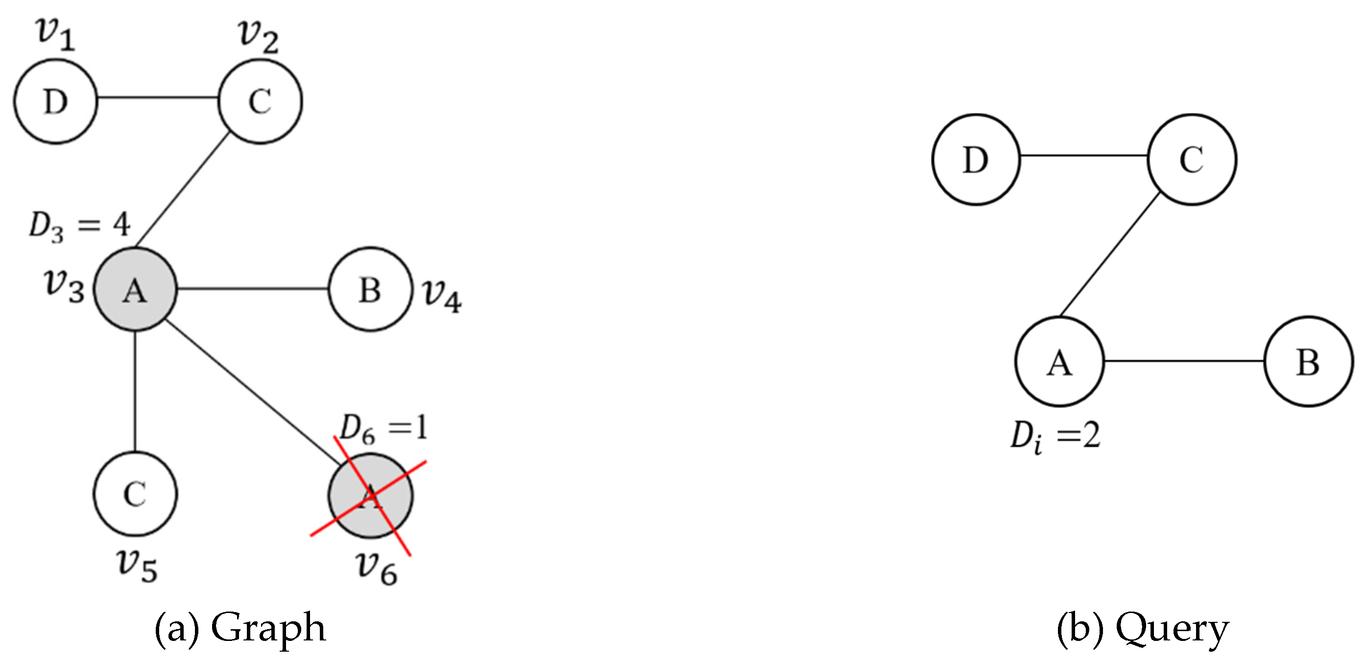
- We predict the filtering score to avoid the vertices that do not need to be searched, based on the statistical information of the graph.
- We determine the search order that determines the priority of the vertices to be searched among the vertices of the query through the filtering score.
- We partition the query into subqueries according to the filtering score for distributed query processing in Spark.
2. Related Work
3. The Proposed Distributed Subgraph Query Processing
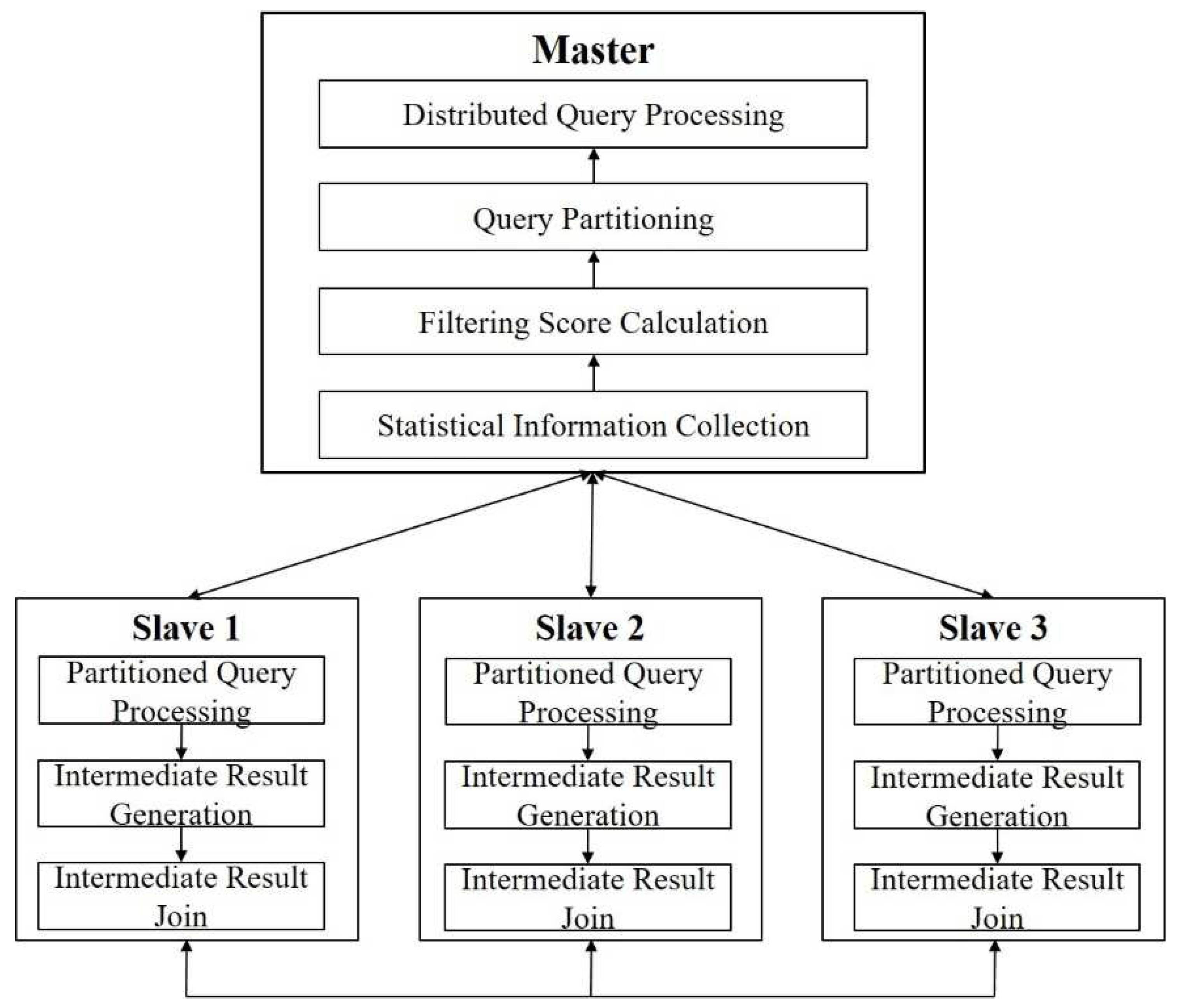
3.1. Overall Architecture
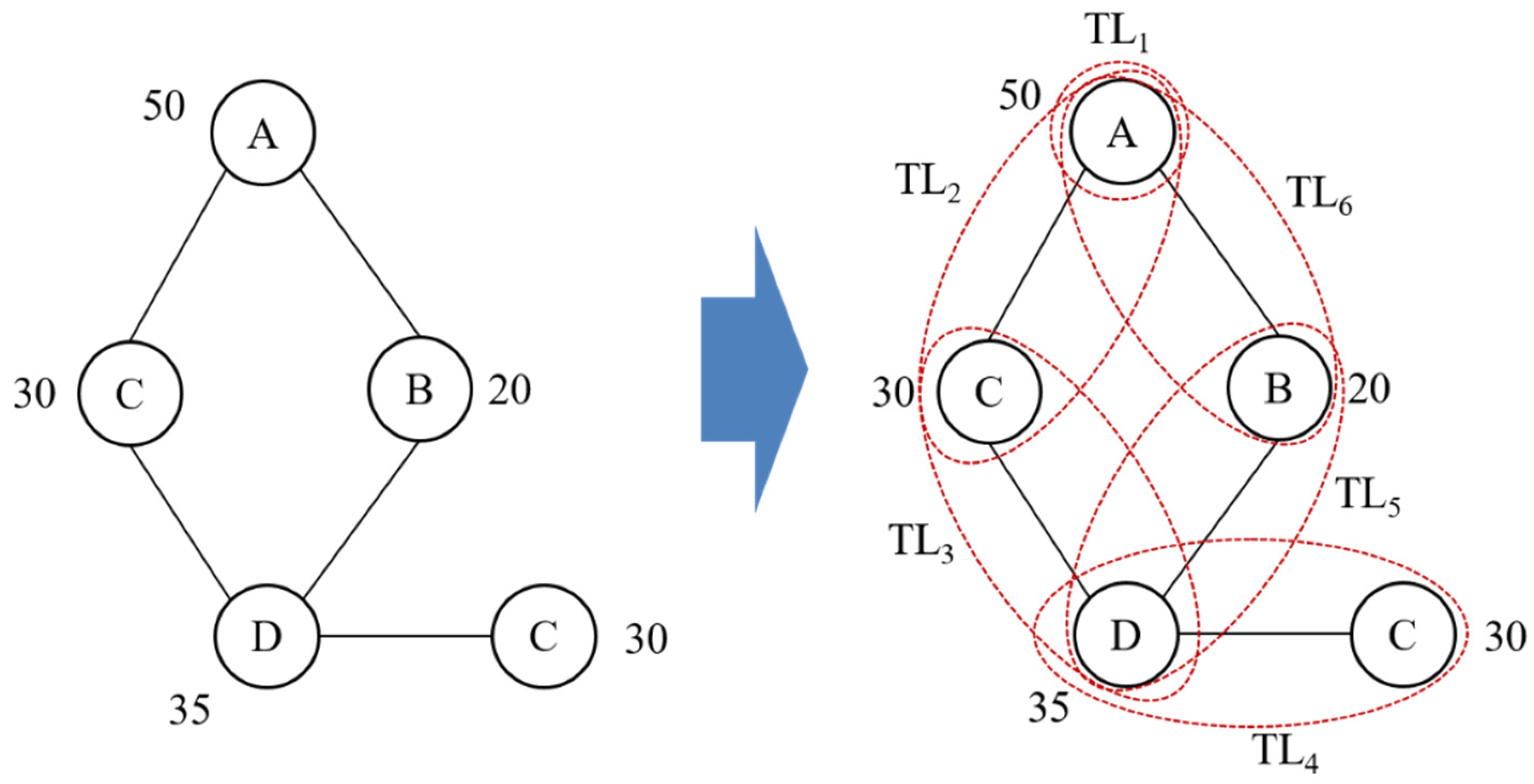
3.2. Filtering Score
3.3. Query partitioning
| Algorithm 1 Query partitioning |
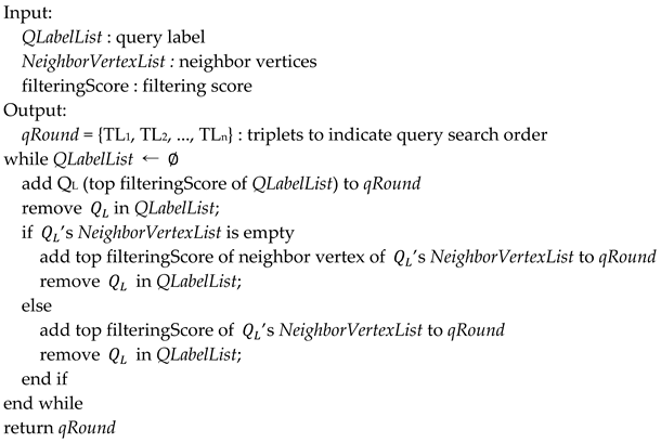 |
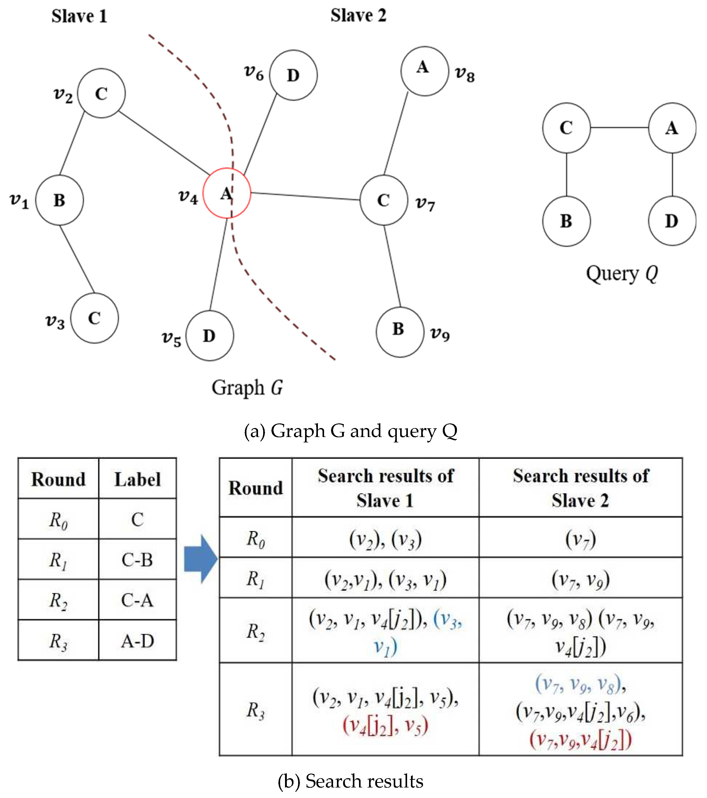
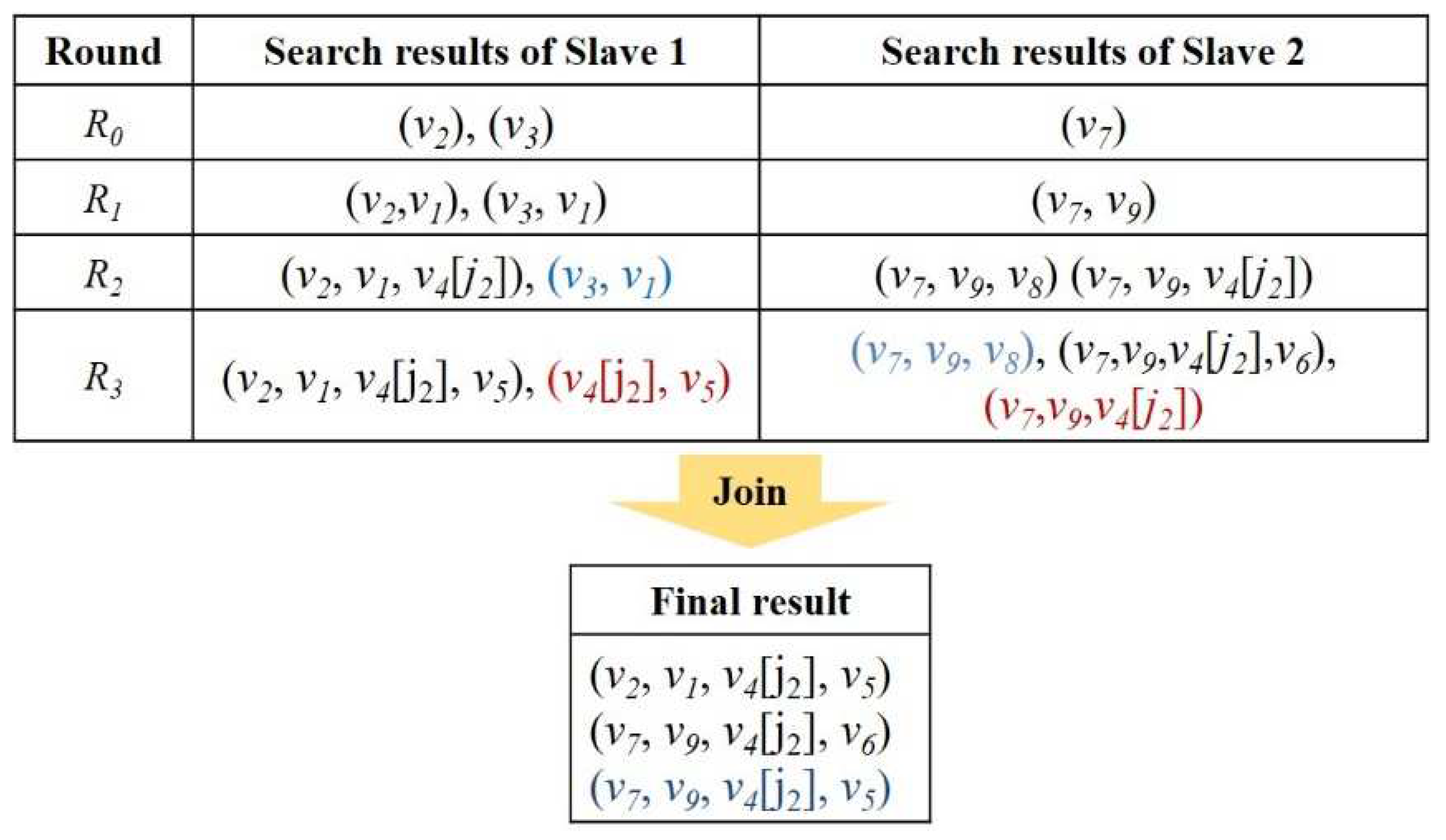
3.4. Distributed Query Processing
| Algorithm 2 Distributed Query Processing |
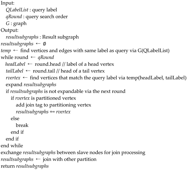 |
4. Performance Evaluation
4.1. Analysis
4.2. Evaluation Results
5. Conclusions
Author Contributions
Funding
Data Availability Statement
Conflicts of Interest
References
- Bok, K.; Jeong, J.; Choi, D.; Yoo, J. Detecting Incremental Frequent Subgraph Patterns in IoT Environments. Sensors 2018, 18, 1–16. [Google Scholar] [CrossRef] [PubMed]
- Bok, K.; Yoo, S.; Choi, D.; Lim, J.; Yoo, J. In-Memory Caching for Enhancing Subgraph Accessibility. Appl. Sci. 2020, 10, 1–18. [Google Scholar] [CrossRef]
- Michail, D.; Kinable, J.; Naveh, B.; Sichi, J.V. JGraphT - A Java Library for Graph Data Structures and Algorithms. ACM Trans. Math. Softw. 2020, 46, 1–29. [Google Scholar] [CrossRef]
- Nguyen, V.; Sugiyama, K.; Nakov, P.; Kan, M. FANG: leveraging social context for fake news detection using graph representation. Commun. ACM 2022, 65, 124–132. [Google Scholar] [CrossRef]
- Saeed, Z.; Abbasi, R.A.; Razzak, M.I.; Xu, G. Event Detection in Twitter Stream Using Weighted Dynamic Heartbeat Graph Approach. IEEE Comput. Intell. Mag. 2019, 14, 29–38. [Google Scholar] [CrossRef]
- Lee, J.; Bae, H.; Yoon, S. Anomaly Detection by Learning Dynamics from a Graph. IEEE Access 2020, 8, 64356–64365. [Google Scholar] [CrossRef]
- anturk, D.; Karagoz, P.; SgWalk: Location Recommendation by User Subgraph-Based Graph Embedding. IEEE Access 2021, 9, 134858–134873. [CrossRef]
- Guo, Q.; Zhuang, F.; Qin, C.; Zhu, H.; Xie, X.; Xiong, H.; He, Q. A Survey on Knowledge Graph-Based Recommender Systems. IEEE Trans. Knowl. Data Eng. 2022, 34, 3549–35646. [Google Scholar] [CrossRef]
- Mukherjee, A.; Chaki, R.; Chaki, N. An Efficient Data Distribution Strategy for Distributed Graph Processing System. In Proceedings of International Conference on Computer Information Systems and Industrial Management, Barranquilla, Colombia, 15-17 July 2022. [Google Scholar]
- Choi, D.; Han, J.; Lim, J.; Han, J.; Bok, K.; Yoo, J. Dynamic Graph Partitioning Scheme for Supporting Load Balancing in Dis-tributed Graph Environments. IEEE Access 2021, 9, 65254–65265. [Google Scholar] [CrossRef]
- Davoudian, A.; Chen, L.; Tu, H.; Liu, M. A Workload-Adaptive Streaming Partitioner for Distributed Graph Stores. Data Sci. Eng. 2021, 6, 163–179. [Google Scholar] [CrossRef]
- Ayall, T.; Liu, H.; Zhou, C.; Seid, A.M.; Gereme, F.B.; Abishu, H.N.; Yacob, Y.H. Graph Computing Systems and Partitioning Techniques: A Survey. IEEE Access 2022, 10, 118523–118550. [Google Scholar] [CrossRef]
- Liu, N.; Li, D.; Zhang, Y.; Li, X. Large-scale graph processing systems: a survey. Frontiers Inf. Technol. Electron. Eng. 2020, 21, 384–404. [Google Scholar] [CrossRef]
- Bouhenni, S.; Yahiaoui, S.; Nouali-Taboudjemat, N.; Kheddouci, H. A Survey on Distributed Graph Pattern Matching in Massive Graphs. ACM Comput. Surv. 2022, 54, 1–35. [Google Scholar] [CrossRef]
- Adoni, W.Y.H.; Tarik, N.; Krichen, M.; El Byed, A. HGraph: Parallel and Distributed Tool for Large-Scale Graph Processing. In Proceedings of International Conference on Artificial Intelligence and Data Analytics, Riyadh, Saudi Arabia, 6-7 April 2021. [Google Scholar]
- Fan, W.; He, T.; Lai, L.; Li, X.; Li, Y.; Li, Z.; Qian, Z.; Tian, C.; Wang, L.; Xu, J.; Yao, Y.; Yin, Q.; Yu, W.; Zeng, K.; Zhao, K.; Zhou, J.; Zhu, D.; Zhu, R. GraphScope: A Unified Engine For Big Graph Processing. Proc. VLDB Endow. 2021, 14, 2879–2892. [Google Scholar] [CrossRef]
- Malewicz, G.; Austern, H.M.; Bik, J.A.; Dehnert, J.; Horn, I.; Leiser, N.; Czajkowski, G.M. Pregel: a system for large-scale graph processing. In Proceedings of ACM SIGMOD International Conference on Management of data, Indianapolis, Indiana, USA, 6-10 June 2010. [Google Scholar]
- Xu, Q.; Wang, X.; Li, J.; Zhang, Q.; Chai, L. Distributed Subgraph Matching on Big Knowledge Graphs Using Pregel. IEEE Access 2019, 7, 116453–116464. [Google Scholar] [CrossRef]
- Dean, J.; Ghemawat, S. MapReduce: Simplified data processing on large clusters. Commun. ACM 2008, 51, 107–113. [Google Scholar] [CrossRef]
- Su, Q.; Huang, Q.; Wu, N.; Pan, Y. Distributed subgraph query for RDF graph data based on MapReduce. Comput. Electr. Eng. 2022, 102, 108221. [Google Scholar] [CrossRef]
- Angles, R.; López-Gallegos, F.; Paredes, R. Power-Law Distributed Graph Generation With MapReduce. IEEE Access 2021, 9, 94405–94415. [Google Scholar] [CrossRef]
- Low, Y.; Gonzalez, J.; Kyrola, A.; Bickson, D.; Guestrin, C.; Hellerstein, J. Distributed GraphLab: A Framework for Machine Learning in the Cloud. Proc. VLDB Endow. 2012, 5, 716–727. [Google Scholar] [CrossRef]
- Gonzalez, J.; Low, Y.; Gu, H.; Bickson, D.; Guestrin, C. PowerGraph: Distributed graph-parallel computation on natural graphs. In Proceedings of USENIX Symposium on Operating Systems Design and Implementation, Hollywood, CA, USA, 8-10 October 2012. [Google Scholar]
- Xin, R.S.; Gonzalez, J.; Michael, F.J.; Ion, S. Graphx: A resilient distributed graph system on spark. In Proceedings of International Workshop on Graph Data Management Experiences and Systems, New York, NY, USA, 24 June 2013. [Google Scholar]
- Zaharia, M.; Xin, R.S.; Wendell, P.; Das, T.; Armbrust, M.; Dave, A.; Meng, X.; Rosen, J.; Venkataraman, S.; Franklin, M.J.; Ghodsi, A.; Gonzalez, J.; Shenker, S.; Stoica, I. Apache spark: a unified engine for big data processing. Commun. ACM 2016, 59, 56–65. [Google Scholar] [CrossRef]
- Talukder, N.; Zaki, M.J. A distributed approach for graph mining in massive networks. Data Min. Knowl. Discov. 2016, 30, 1024–1052. [Google Scholar] [CrossRef]
- Tian, Y.; McEachin, R.C.; Santos, C.; States, D.J.; Patel, J.M. SAGA: a subgraph matching tool for biological graphs. Bioinform. 2006, 23, 232–239. [Google Scholar] [CrossRef] [PubMed]
- Zhu, L.; Yao, Y.; Wang, Y.; Hei, X.; Zhao, Q.; Ji, W.; Yao, Q. A novel subgraph querying method based on paths and spectra. Neural Comput. Appl. 2019, 31, 5671–5678. [Google Scholar] [CrossRef]
- Liang, Y.; Zhao, P. Workload-Aware Subgraph Query Caching and Processing in Large Graphs. In Proceedings of IEEE International Conference on Data Engineering, Macao, China, 8-11 April 2019. [Google Scholar]
- 30-22. Sun, S.; Luo, Q. 11 April 2019, 30-22. Sun, S.; Luo, Q. Scaling Up Subgraph Query Processing with Efficient Subgraph Matching. In Proceedings of IEEE International Conference on Data Engineering, Macao, China, 8-11 April 2019.
- Luaces, D.; Viqueira, J.R.R.; Cotos, J.M.; Flores, J.C. Efficient access methods for very large distributed graph databases. Inf. Sci. 2021, 573, 65–81. [Google Scholar] [CrossRef]
- Cheng, J.; Ke, Y.; Ng, W. Efficient query processing on graph databases. ACM Trans. Database Syst. 2009, 34, 1–48. [Google Scholar] [CrossRef]
- Wang, J.; Ntarmos, N.; Triantafillou, P. GraphCache: a caching system for graph queries. In Proceedings of International Conference on Extending Database Technology, Venice, Italy, 21-24 March 2017. [Google Scholar]
- Li, Y.; Yang, Y.; Zhong, Y. An Incremental Partitioning Graph Similarity Search Based on Tree Structure Index. In Proceedings of International Conference of Pioneering Computer Scientists, Engineers and Educators, Taiyuan, China, 18-21 September 2020. [Google Scholar]
- Wangmo, C.; Wiese, L. Efficient Subgraph Indexing for Biochemical Graphs. In Proceedings of International Conference on Data Science, Technology and Applications, Lisbon, Portugal, 11-13 July 2022. [Google Scholar]
- Khuller, S.; Raghavachari, B.; Young, N. Balancing minimum spanning trees and shortest-path trees. Algorithmica 1995, 14, 305–321. [Google Scholar] [CrossRef]
- Balaji, J.; Sunderraman, R. Distributed Graph Path Queries Using Spark. In Proceedings of Annual Computer Software and Applications Conference, Atlanta, GA, USA, 10-14 June 2016. [Google Scholar]
- Wei, F. TEDI: efficient shortest path query answering on graphs. In Proceedings of ACM SIGMOD International Conference on Management of Data, Indianapolis, Indiana, USA, 6-10 June 2010. [Google Scholar]
- Cordella, L.P.; Foggia, P.; Sansone, C.; Vento, M. A (sub)graph isomorphism algorithm for matching large graphs. IEEE Trans. Pattern Anal. Mach. Intell. 2004, 26, 1367–1372. [Google Scholar] [CrossRef]
- He, H.; Singh, A.K. Graphs-at-a-time: query language and access methods for graph databases. In Proceedings of ACM SIGMOD International Conference on Management of Data, Vancouver, BC, Canada, 10-12 June 2008. [Google Scholar]
- Zhang, S.; Li, S.; Yang, J. GADDI: distance index based subgraph matching in biological networks. In Proceedings of Inter-national Conference on Extending Database Technology, Saint Petersburg, Russia, 24-26 March 2009. [Google Scholar]
- Ullmann, J.R. An algorithm for subgraph isomorphism. J. ACM 1976, 23, 31–42. [Google Scholar] [CrossRef]
- Zhang, X.; Chen, L. Distance-aware selective online query processing over large distributed graphs. Data Sci. Eng. 2017, 2, 2–21. [Google Scholar] [CrossRef]
- Jing, N.; Huang, Y.W.; Rundensteiner, E.A. Hierarchical encoded path views for path query processing: An optimal model and its performance evaluation. IEEE Trans. Knowl. Data Eng. 1998, 10, 409–432. [Google Scholar] [CrossRef]
- Zaharia, M.; Xin, R.S.; Wendell, P.; Das, T.; Armbrust, M.; Dave, A.; Meng, X.; Rosen, F.; Venkataraman, S.; Franklin, M.J.; Ghodsi, A.; Gonzalez, J.; Shenker, S.; Stoica, I. Apache Spark: a unified engine for big data processing. Commun. ACM 2016, 59, 56–65. [Google Scholar] [CrossRef]
- Ammar, K.; McSherry, F.; Salihoglu, S.; Joglekar, M. Distributed Evaluation of Subgraph Queries Using Worst-case Optimal and Low-Memory Dataflows. Proc. VLDB Endow. 2018, 11, 691–704. [Google Scholar] [CrossRef]
- Fathimabi, S.; Subramanyam, R B. V.; Somayajulu, D.V.L.N. MSP: Multiple Sub-graph Query Processing using Structure-based Graph Partitioning Strategy and Map-Reduce. J. King Saud Univ. Comput. Inf. Sci. 2019, 31, 22–34. [Google Scholar]
- Cheng, J.; Ke, Y.; Fu, A.W.; Yu, J.X. Fast graph query processing with a low-cost index. VLDB J. 2021, 20, 521–539. [Google Scholar] [CrossRef]
- Sala, A.; Zheng, H.; Zhao, B.Y.; Gaito, S.; Rossi, G.P. Brief announcement: revisiting the power-law degree distribution for social graph analysis. In Proceedings of Annual ACM Symposium on Principles of Distributed Computing, Zurich, Switzerland, 5-28 July 2010. [Google Scholar]
- Zhang, S.; Jiang, Z.; Hou, X.; Li, M.; Yuan, M.; You, H. DRONE: An Efficient Distributed Subgraph-Centric Framework for Processing Large-Scale Power-law Graphs. IEEE Trans. Parallel Distributed Syst. 2023, 34, 463–474. [Google Scholar] [CrossRef]
- Faloutsos, M.; Faloutsos, P.; Faloutsos, C. On power-law relationships of the internet topology. ACM SIGCOMM Comput. Commun. Rev. 1999, 29, 251–262. [Google Scholar] [CrossRef]
- Goldstein, M.L.; Morris, S.A.; Yen, G.G. Problems with fitting to the power-law distribution. Eur. Phys. J. B. 2005, 41, 255–258. [Google Scholar] [CrossRef]
- Stanford Large Network Dataset Collection, Available online:. Available online: https://snap.stanford.edu/data (accessed on 15 January 2021).
- GTgraph, Available online:. Available online: http://www.cse.psu.edu/~kxm85/software/GTgraph (accessed on 5 October 2021).
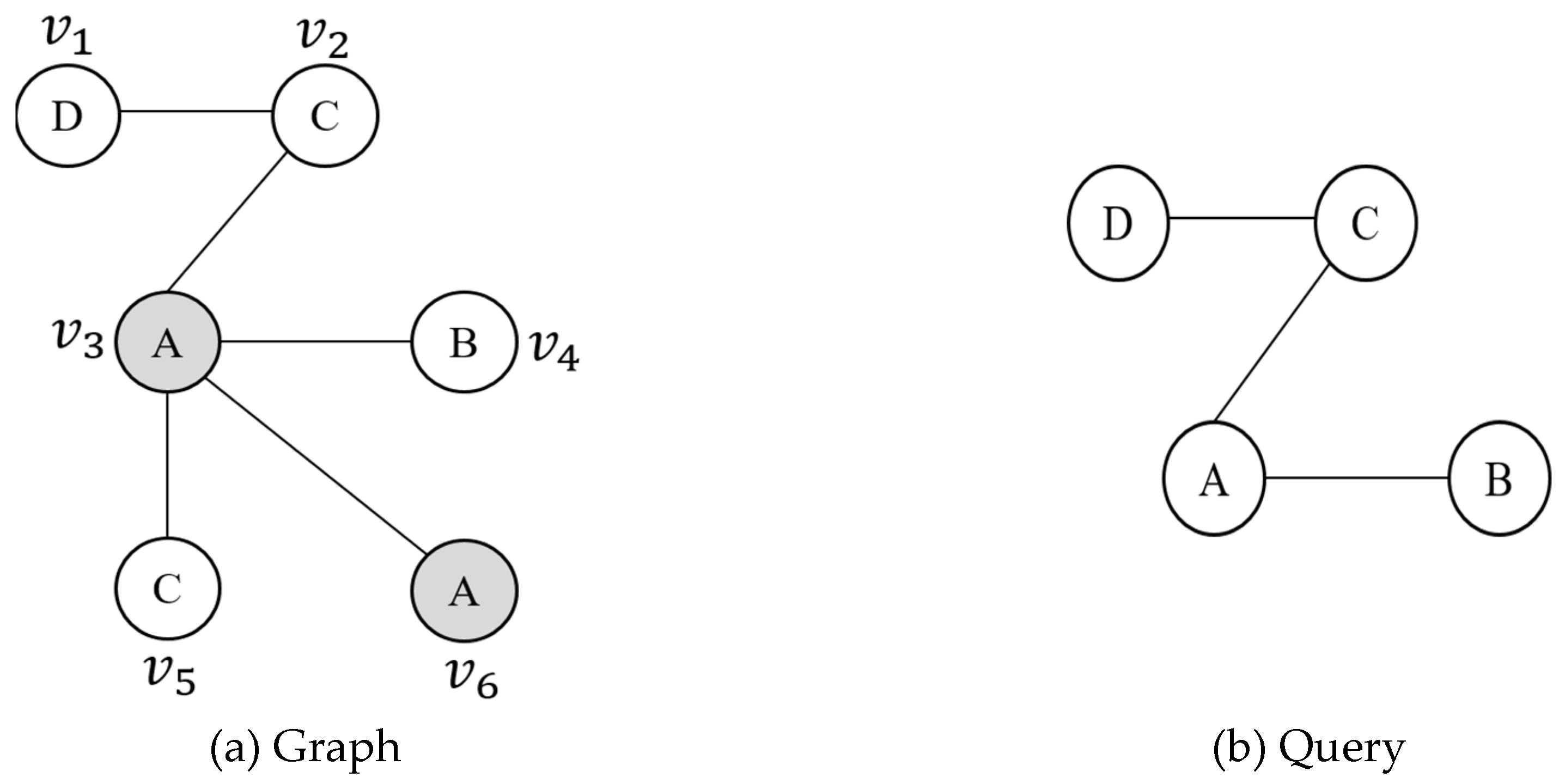
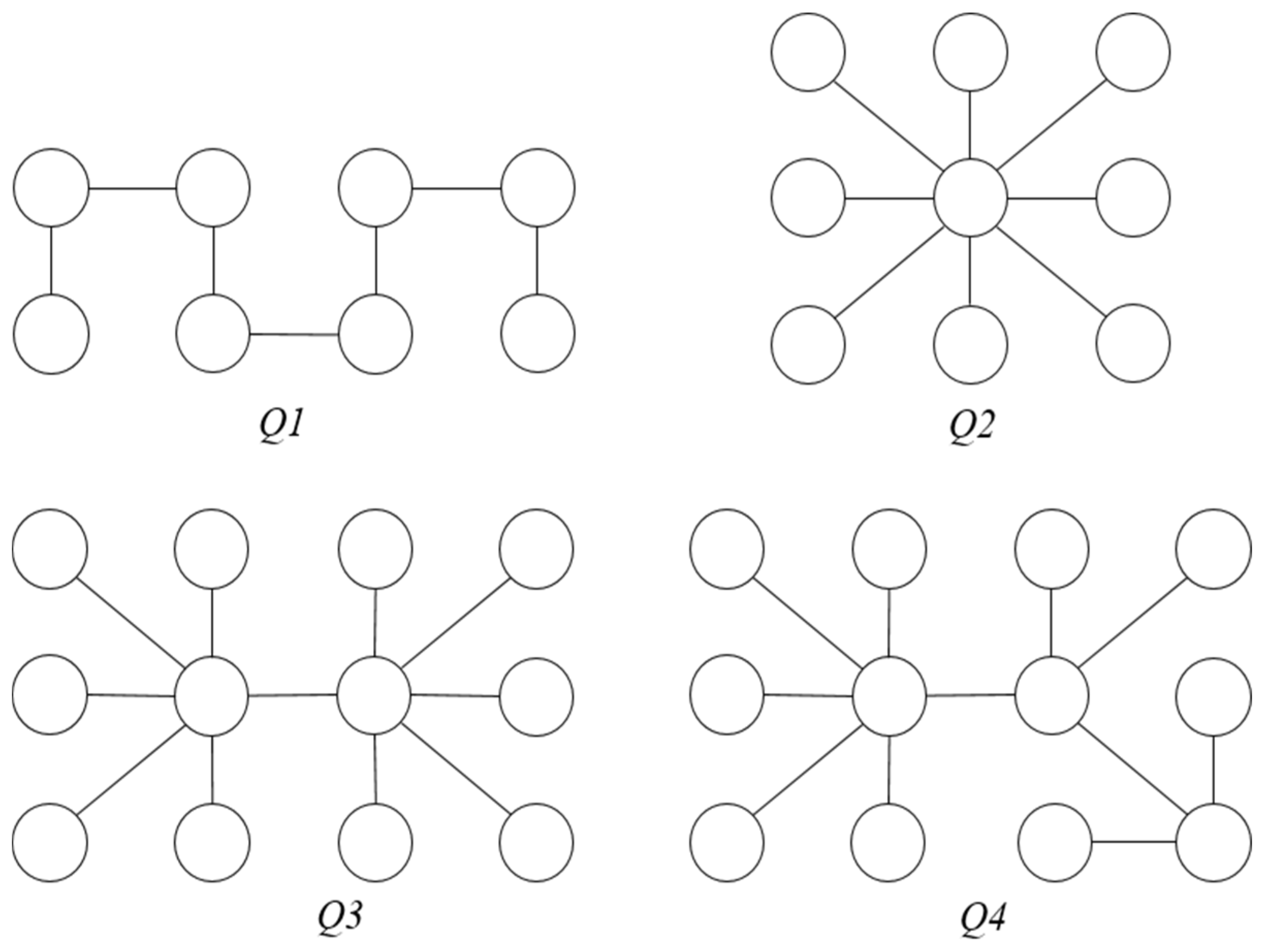
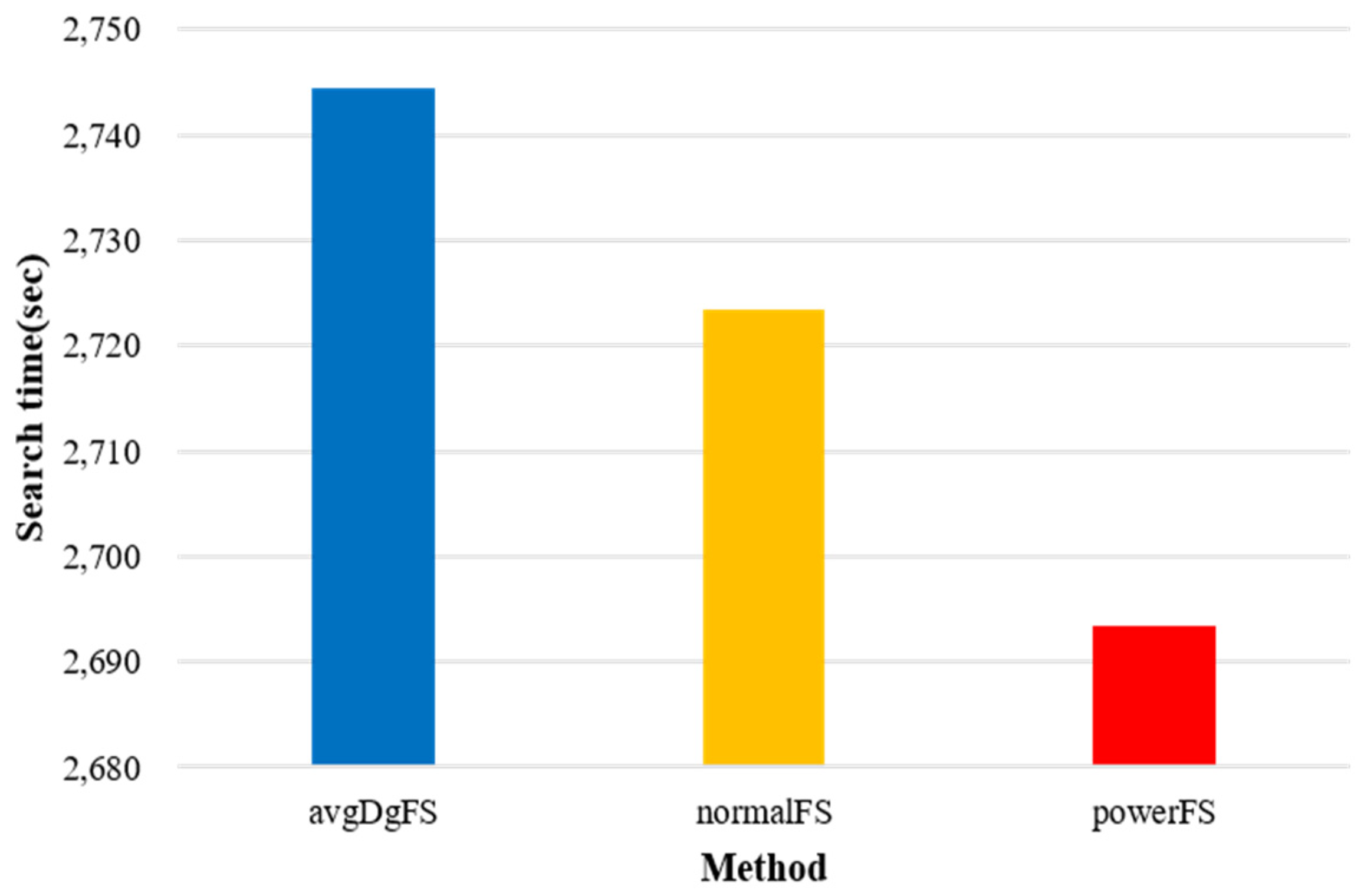
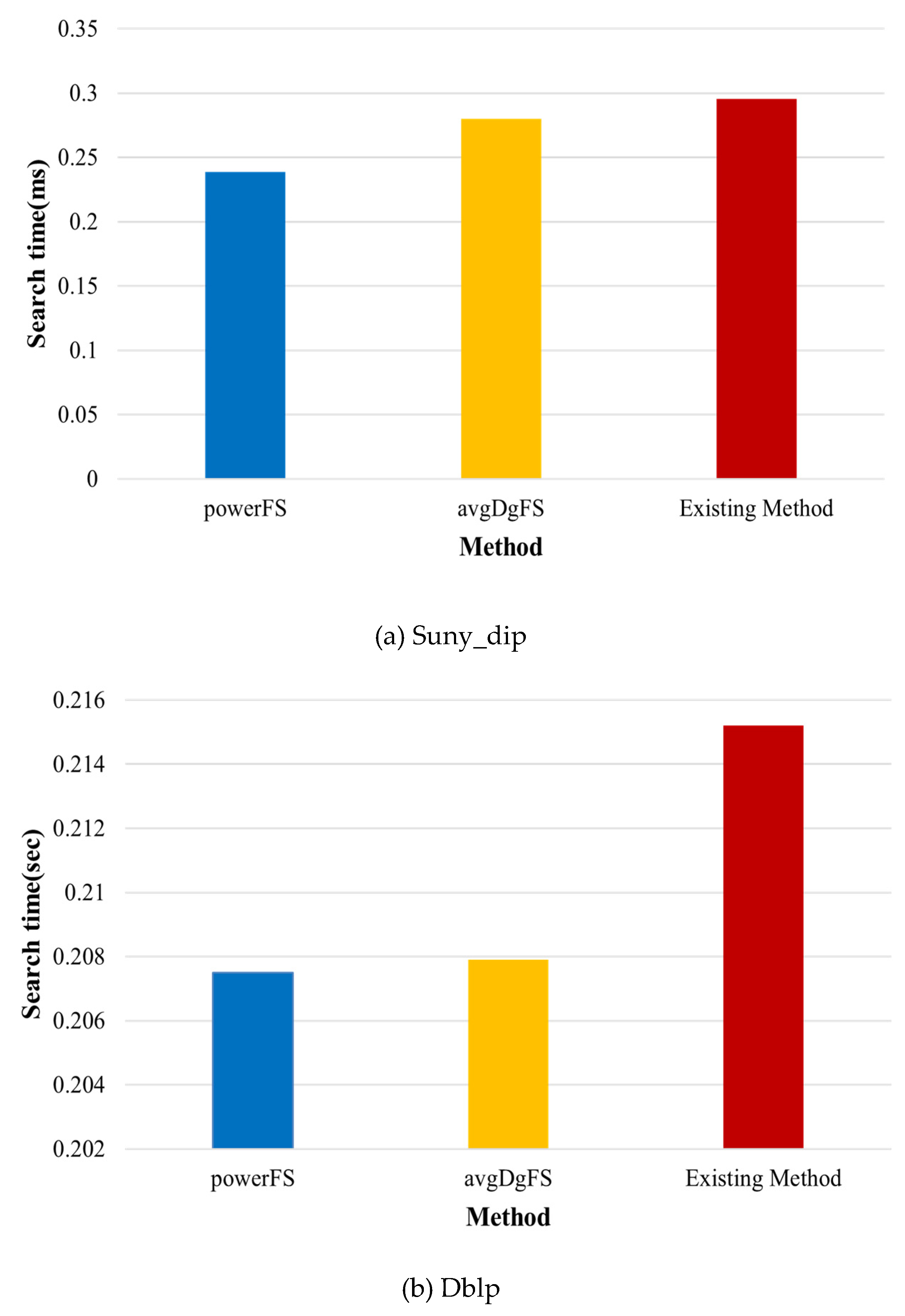
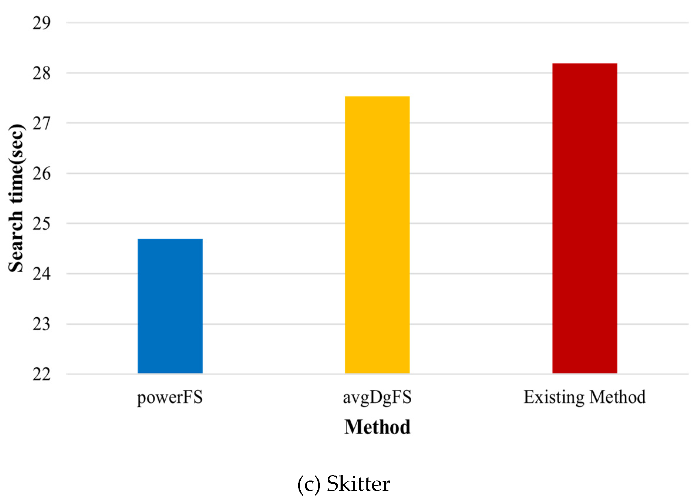
| Parameters | Description |
|---|---|
| Filtering probability of normal distribution | |
| Filtering probability of power-law distribution | |
| Number of vertices with label in graph | |
| Total number of vertices in graph | |
| Average degree of collected labels |
| Schemes | Methodology | Environment | Query Type | index | Verification | Search Order |
|---|---|---|---|---|---|---|
| GraphCache[33] | FAV | Single | Random | , | 0 | X |
| MSP[47] | FAV | Hadoop | Random | IGI | 0 | X |
| HGraph[15] | - | Hadoop, Spark | Random | - | - | X |
| DWJ[46] | Path | Timely Dataflow | Directed | Edge index | X | X |
| SPQ[37] | Path | Spark | Random | X | X | X |
| Proposed | Path | Spark | Random | X | X | Filtering score |
| Parameter | Value |
|---|---|
| Processor | Intel(R) Core(TM) i7-6700 CPU 3.40GHz |
| Memory | 30G |
| Number of clusters | 3 |
| Programming language | Scala |
| Dataset | Vertices | Edges | Description |
|---|---|---|---|
| suny_dip | 22,596 | 69,148 | Biology data |
| dblp | 425,961 | 1,049,866 | Coauthor network |
| skitter | 1,696,415 | 11,095,298 | Internet topology |
| GTgraph | 1,696,415 | 11,095,298 | Randomly generated graph |
Disclaimer/Publisher’s Note: The statements, opinions and data contained in all publications are solely those of the individual author(s) and contributor(s) and not of MDPI and/or the editor(s). MDPI and/or the editor(s) disclaim responsibility for any injury to people or property resulting from any ideas, methods, instructions or products referred to in the content. |
© 2023 by the authors. Licensee MDPI, Basel, Switzerland. This article is an open access article distributed under the terms and conditions of the Creative Commons Attribution (CC BY) license (http://creativecommons.org/licenses/by/4.0/).


