Landslide Susceptibility Mapping: Analysis of Different Feature Selection Techniques with Artificial Neural Network Tuned by Bayesian and Metaheuristic Algorithms

Preprint

Article

Landslide Susceptibility Mapping: Analysis of Different Feature Selection Techniques with Artificial Neural Network Tuned by Bayesian and Metaheuristic Algorithms

Altmetrics

Downloads

152

Views

Comments

A peer-reviewed article of this preprint also exists.

This version is not peer-reviewed

Submitted:

20 July 2023

Posted:

26 July 2023

You are already at the latest version

Alerts

Abstract

The most frequent, noticeable, and frequent natural calamity in the karakoram region is landslides. Extreme landslides have occurred frequently along Karakoram highway, particularly during the monsoon, causing a major loss of life and property. Therefore, it was necessary to look for a solution to increase growth and vigilance in order to lessen losses related to landslides caused by natural disasters. By utilizing contemporary technologies, an early warning system might be developed. Artificial neural networks (ANNs) are widely used nowadays across many industries. This paper's major goal is to provide new integrative models for assessing landslide susceptibility in a prone area of north of Pakistan. To do this, the training of an artificial neural network (ANN) is supervised using metaheuristic and Bayesian techniques: particle swarm optimization algorithm (PSO), Genetic algorithm (GA), Bayesian optimization Gaussian process (BO_GP), and Bayesian optimization Gaussian process (BO_TPE). 304 previous landslides and the eight most prevalent conditioning elements combine to form a geographical database. The models are hyper-parameter optimized, and the best ones are employed to generate the susceptibility maps. The area under the receiving operating characteristic curve (AUROC) accuracy index found demonstrated that the maps produced by both Bayesian and metaheuristic algorithms are highly accurate. The effectiveness and efficiency of applying artificial neural networks (ANNs) for landslide mapping, susceptibility analysis, and forecasting are studied in this research it’s observed from experimentation that the performance differences for GA, BO_GP, and PSO compared to BO_TPE are relatively small, ranging from 0.3166% to 1.8399%. This suggests that these techniques achieved comparable performance to BO_TPE in terms of AUC. However, it's important to note that the significance of these differences can vary depending on the specific context and requirements of the ML task. Additionally in this study, we explore eight feature selection algorithms to determine the geospatial variable importance for landslide susceptibility mapping along the KKH. The algorithms considered include Information Gain, Gain Ratio, OneR Classifier, Subset Evaluators, Principal Components, Relief Attribute Evaluator, Correlation, and Symmetrical Uncertainty. These algorithms enable us to evaluate the relevance and significance of different geospatial variables in predicting landslide susceptibility. By applying these feature selection algorithms, we aim to identify the most influential geospatial variables that contribute to landslide occurrences along the KKH. The algorithms encompass a diverse range of techniques, such as measuring entropy reduction, accounting for attribute bias, generating single rules, evaluating feature subsets, reducing dimensionality, and assessing correlation and information sharing. The findings of this study will provide valuable insights into the critical geospatial variables associated with landslide susceptibility along the KKH. These insights can aid in the development of effective landslide mitigation strategies, infrastructure planning, and targeted hazard management efforts. Additionally, the study contributes to the field of geospatial analysis by showcasing the applicability and effectiveness of various feature selection algorithms in the context of landslide susceptibility mapping.

Keywords:

Subject: Computer Science and Mathematics - Artificial Intelligence and Machine Learning

Study area

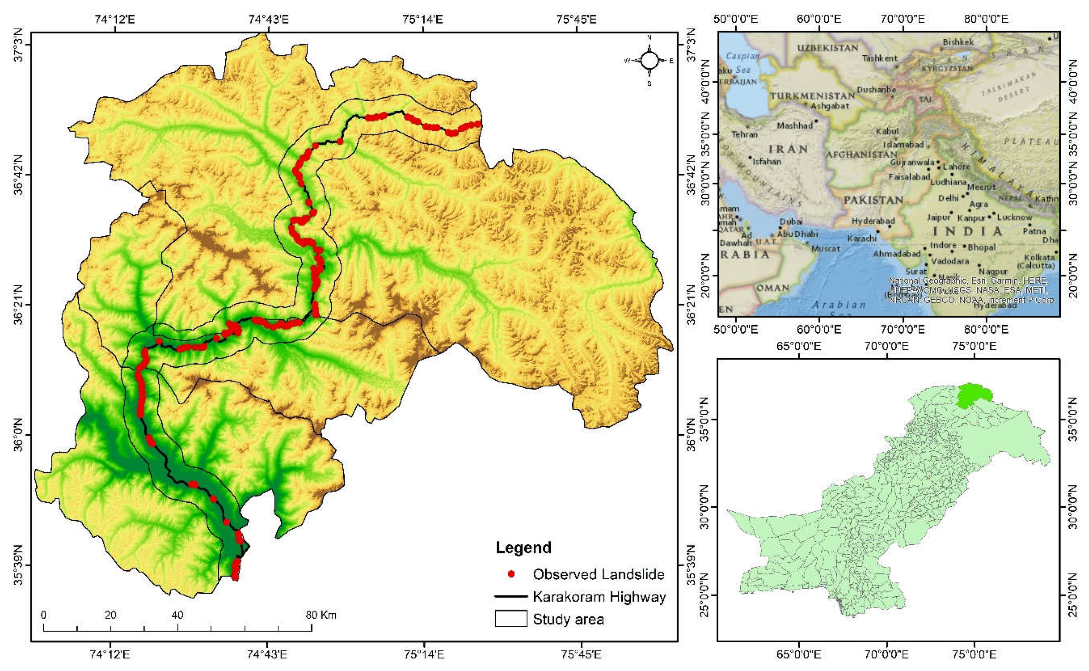
We conducted a study in the northern part of Pakistan, focusing on an approximately 332 km stretch of the KKH highway. The KKH highway is a major road that spans 1300 km, connecting various provinces of Pakistan, namely Punjab, Khyber Pakhtunkhwa, and Gilgit Baltistan, with Xinjiang, an autonomous region of China. Our study specifically covered the Gilgit, Hunza, and Nagar districts. Along the KKH, there are several villages including Juglot (located between 36°12′147″N latitude and 74°18′772″E longitude), Jutal, Rahimbad, Aliabad, and others, ultimately reaching Khunjarab Top, which serves as the border crossing between China and Pakistan. This region is situated alongside the Indus River, Hunza River, and Gilgit River. The majority of the region consists of mountainous terrain, with its highest point reaching an elevation of 5370 m and the lowest point at 1210 m. Common natural hazards in this area include snow avalanches, landslides, and earthquakes.

Figure 1. Study area of our experiment.

1. Introduction

Artificial neural networks are utilized to solve a range of issues in industries like banking, manufacturing, electronics, and medicine, among others [1]. The backpropagation approach is typically used to train neural networks [2,3]. The backpropagation method can be trained using a variety of algorithms, including gradient descent, conjugate gradient descent, robust, BFGS quasi-Newton, one-step secant, Levenberg-Marquardt, and Bayesian regularization [4].Some characteristics, such as the number of hidden layers and the number of neurons in each layer, must be defined during the design and training of an ANN; these aspects vary depending on the particular application. There isn't a standard, clear approach for selecting these settings. It is utilized in a way that is almost like trial and error, but it requires more computing time and is not very accurate. Therefore, it is required to propose a method to choose the ideal set of parameters that will have the greatest impact on ANN performance.

From the literature, it can be inferred that metaheuristic optimization algorithms have effectively been employed to overcome the computing limitations of traditional landslide predictive models, hence enhancing their performance. The local minimum trap could become a barrier to precise estimations when it comes to ANNs. But recent research has demonstrated that using metaheuristic techniques, such computational problems can be resolved [5].Testing novel metaheuristic methods is an important step toward discovering more efficient models, but, as well-known optimizers (such as the PSO and GA) have been sufficiently evaluated. This study's main objective is to assess the effectiveness of four optimization strategies—particle swarm optimization algorithm (PSO), Genetic algorithm (GA), Bayesian optimization Gaussian process (BO-GP), and Bayesian optimization Gaussian process (BO-TPE) —in combination with artificial neural networks (ANN) to produce a map of the KKH region's susceptibility to landslides in northern areas of Pakistan [6,7,8,9] and we also try to explore eight different techniques to evaluate the importance of geospatial variables used in our case study these feature selection techniques will help us identify the most important and relevant feature that should be used based on different evaluation criteria.

In the context of artificial neural networks (ANNs), optimization algorithms such as particle swarm optimization (PSO), genetic algorithm (GA), and Bayesian optimization have been widely used to improve the performance of ANNs in various classification tasks [10,11,12,13]. Here are some specific examples of their applications in the context of ANNs for data classification:

Particle Swarm Optimization (PSO) for ANN

1.: PSO has been used to optimize the weights and biases of the ANN to improve its classification accuracy. By searching the weight space, PSO helps to find the optimal set of weights that minimize the prediction error and maximize the classification performance.
2.: PSO has been applied to optimize the architecture of the ANN, including the number of hidden layers and the number of neurons in each layer. It helps to determine the optimal network structure that suits the complexity of the classification problem.

Genetic Algorithm (GA) for ANN

1.: GA has been used to train ANNs by adjusting the weights and biases of the network. By applying genetic operators such as crossover and mutation, GA explores the search space of weight configurations to find the best set of weights that lead to improved classification accuracy.
2.: GA has been employed to optimize the architecture of the ANN, including the number of hidden layers and neurons. By evolving populations of networks with different architectures, GA helps to identify the optimal network structure that achieves better classification performance.

Bayesian Optimization for ANN

1.: Bayesian optimization has been used to optimize the hyperparameters of ANNs, such as learning rate, regularization strength, and network architecture. By leveraging Bayesian inference, it explores the hyperparameter space to find the optimal configuration that maximizes the classification accuracy.
2.: Bayesian optimization has been applied to tune the activation functions, dropout rates, and other architectural choices of ANNs. It helps to identify the best combinations of these hyperparameters that result in improved classification performance.

In all these cases, the optimization algorithms (PSO, GA, and Bayesian optimization) play a crucial role in training and fine-tuning ANNs for data classification. They help to search for optimal weights, biases, and hyperparameter configurations, allowing ANNs to achieve higher accuracy and better generalization in classification tasks [14,15,16,17,18].

By tuning the weights and biases, these algorithms supervise the performance of the ANN in predicting the landslide susceptibility index (LSI). In the context of predicting landslide susceptibility using artificial neural networks (ANNs), the weights and biases of the network are adjusted or tuned by the optimization algorithms (such as genetic algorithms, particle swarm optimization, or Bayesian optimization) to improve the performance of the ANN in predicting the landslide susceptibility index (LSI).The weights and biases in an ANN determine the strength and influence of connections between neurons in different layers. By adjusting these parameters, the ANN can learn and adapt to the patterns and relationships present in the input data, in this case, the conditioning elements used to assess landslide susceptibility.

During the training phase, the optimization algorithms iterate through different combinations of weights and biases, evaluating the performance of the ANN based on a defined metric (e.g., accuracy, area under the curve). The algorithms aim to find the set of weights and biases that minimize the prediction error or maximize the performance metric, ultimately leading to a more accurate prediction of the LSI.

The optimization algorithms use various strategies, such as gradient descent, genetic operators (crossover and mutation), or probabilistic modeling, to explore the search space of weight and bias combinations [19,20,21,22,23]. Through iterations and feedback from evaluating the ANN's predictions, the algorithms progressively adjust the weights and biases to converge towards an optimal solution that yields the best performance in predicting the LSI.

By continuously fine-tuning the weights and biases, these optimization algorithms guide the ANN to learn and generalize patterns from the training data, enabling the model to make more accurate predictions of landslide susceptibility based on the conditioning elements. This iterative optimization process helps to improve the effectiveness of the ANN in capturing the complex relationships between the input features and the LSI, leading to more reliable and accurate predictions of landslide susceptibility.

In addition to discuss the fine tuning of ANN using metaheuristic and Bayesian algorithms this study, also address the challenge of identifying the geospatial variable importance for landslide susceptibility mapping. To achieve this, we employ eight different feature selection algorithms: Information Gain, Variance Inflation Factor , OneR Classifier, Subset Evaluators, Principal Components, Relief Attribute Evaluator, Correlation, and Symmetrical Uncertainty. Each algorithm brings a unique approach to assessing the relevance and significance of geospatial variables in predicting landslide occurrences.

The selection of these feature selection algorithms offers a comprehensive evaluation of different approaches to geospatial variable importance assessment. By leveraging these algorithms, we aim to uncover the most influential variables that contribute to landslide susceptibility mapping in our case study. This study not only contributes to the specific context of landslide susceptibility mapping along the KKH but also has broader implications for geospatial analysis and hazard management. The findings will enhance our understanding of the geospatial factors influencing landslide occurrences and serve as a foundation for future research and development of effective strategies to reduce landslide risks in mountainous regions.

Analyzing feature selection algorithms helps in identifying the most important geospatial variables for landslide susceptibility mapping. This deepens our understanding of the specific factors that contribute to landslide occurrences along the Karakoram Highway (KKH) in Pakistan. By uncovering the key variables, we can gain valuable insights into the underlying mechanisms and processes that influence landslide susceptibility. By determining the geospatial variable importance, we can refine landslide prediction models and improve the accuracy of landslide susceptibility maps. Focusing on the most relevant variables allows us to develop more precise and reliable mapping methodologies. This, in turn, enables better hazard assessment, infrastructure planning, and land management decisions along the KKH.

Analyzing geospatial variable importance helps in proactive hazard management along the KKH. With a better understanding of the critical variables, authorities and stakeholders can implement targeted measures to minimize the risks associated with landslides. This includes implementing early warning systems, designing effective slope stabilization measures, and adopting appropriate land use planning strategies. By identifying the most influential geospatial variables, analyzing feature selection algorithms enables optimal resource allocation for landslide mitigation efforts. Instead of allocating resources uniformly across all variables, decision-makers can prioritize and allocate resources to monitor, manage, and mitigate the variables that have the greatest impact on landslide susceptibility. This ensures efficient utilization of limited resources for effective hazard management.

In summary, analyzing feature selection algorithms for geospatial variable importance in the context of landslide susceptibility mapping along the KKH offers several benefits. It enhances our understanding of landslide mechanisms, improves prediction and mapping accuracy, facilitates proactive hazard management, optimizes resource allocation, informs infrastructure planning, and provides valuable insights for broader geospatial analysis tasks. These benefits contribute to safer infrastructure, reduced risks, and more effective decision-making for landslide-prone areas. Overall, by combining advanced feature selection algorithms with geospatial analysis, this study aims to provide a comprehensive understanding of the geospatial variable importance for landslide susceptibility mapping along the KKH, ultimately contributing to safer infrastructure and improved hazard management in the region.

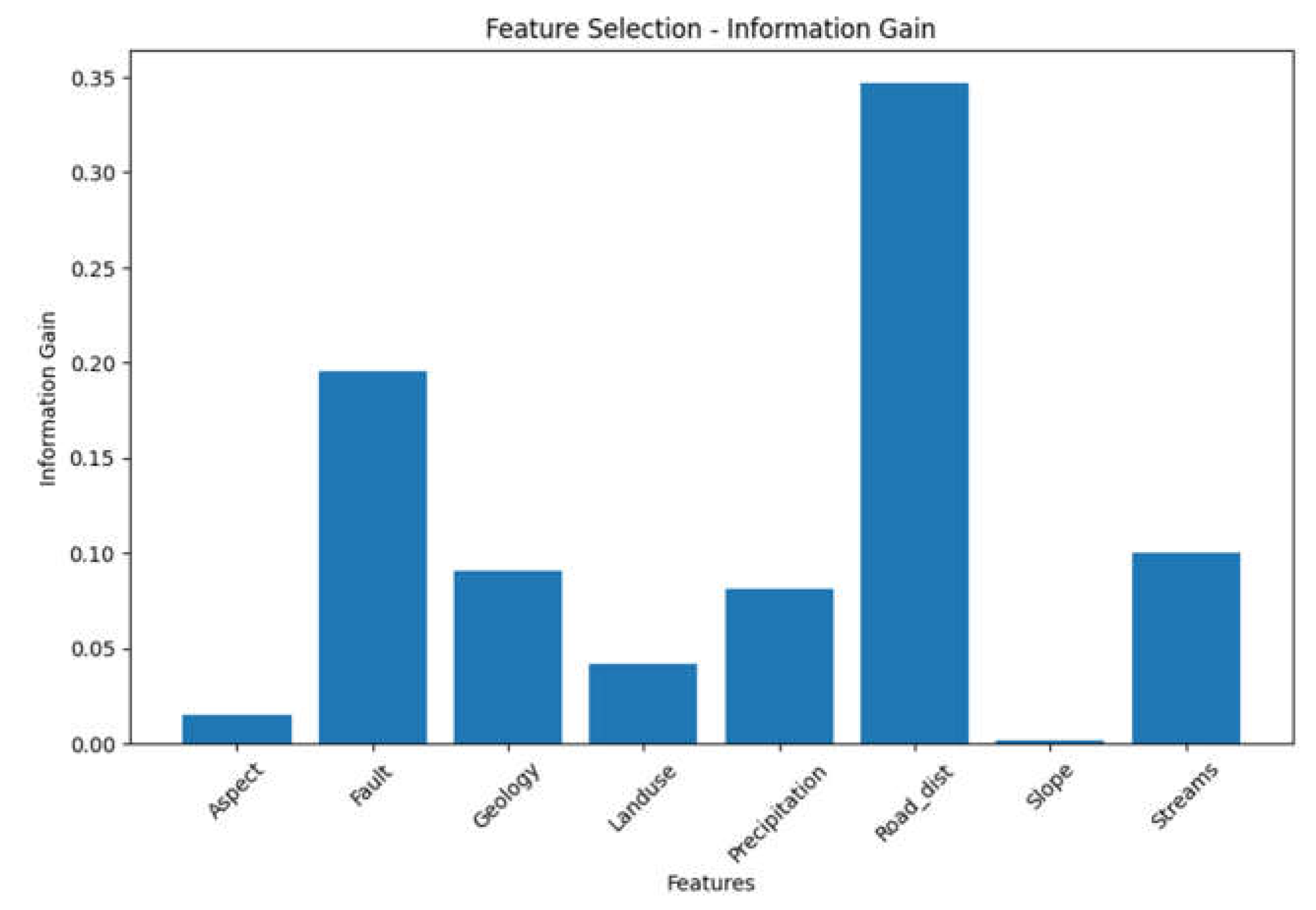
Based on our feature selection analysis. We can declare distance to the road , Faults and Streams as the most influential factors because of following reasons. "Road_dist" demonstrates several characteristics that indicate its significance. It has the highest information gain, low multicollinearity (low VIF), high accuracy scores in the OneR classifier, inclusion in high-accuracy feature combinations, and relatively high importance scores in the Relief Attribute Evaluator and Symmetrical Uncertainty. Therefore, "Road_dist" can be considered as one of the most influential factors. And it can also be evident from ground survey as the roads are constructed in harsh mountainous train with improper blasting that make the slope very venerable near the road and most of landslide occur near roads. The second most influential factor that we identified from our analysis is "Fault” this factor appears in multiple tables with notable characteristics. It has relatively high information gain, moderate importance scores, and is included in high-accuracy feature combinations in the Subset Evaluator table. While it may not be as consistently influential as "Road_dist," it still demonstrates significance in the analysis. And this fact can also be evident from ground survey that highlight the fact that most landslide happened around the region near fault lines. "Streams" this factor also appears in multiple tables, showing relatively high information gain and being included in high-accuracy feature combinations. It demonstrates importance in the analysis, although to a lesser extent compared to "Road_dist" and "Fault." Again this phenomena can be verified from our case study where most of the land is irrigated from the streams emerge from rivers that are filled with water from melting snow and glaciers from high mountains and even the man made stream channel make the region more venerable for landslides. Other features while not as consistently influential as the three factors mentioned above, several other features show importance in specific tables. For example, "Geology" and "Aspect" have relatively high importance scores in the Relief Attribute Evaluator table, and "Landuse" has notable importance in the Subset Evaluator table.

It's important to note that the level of influence may vary depending on the specific analysis techniques and evaluation measures used in the tables. Additionally, the interpretation of influence should consider the context and objectives of the analysis. Further analysis, considering the dataset and specific requirements, is recommended to finalize the most influential factors for the specific task at hand. As we discuss earlier that reducing the entropy and result into information loss and important patterns can be loss [24] therefore and we keep all the variable because the information gain for all of them was greater than zero.

Architecture of artificial neural network

The architecture of the artificial neural network (ANN) for landslide susceptibility mapping can be described as. The input layer of the ANN receives the relevant data or features related to landslide susceptibility in the KKH region. These features may include factors such as geological characteristics, slope angles, aspect, geological properties, and land cover. The number of neurons specific settings such as activation function, batch size, and epochs for each technique determined during the design and training of the ANN for BO_GP, BO_TPE, PSO and GA are mentioned in table below.

Table 1. The information given includes the hyperparameters related to the optimization techniques (PSO, GA, BO_GP, and BO_TPE).

HOP Technique	Activation	Batch_size	Epochs	Neurons
PSO	1.7421875	0.3671875	40.2734375	95.4296875
GA	sgd	16	50	64
BO_GP	tanh	16	47	54
BO_TPE	1	16.0	50.0	80.0

The activation function is a crucial component of ANNs, as it introduces non-linearity and affects the network's ability to model complex relationships. The table provides information about the activation functions used for each technique, such as "sgd," "tanh," and the value "1.7421875" for PSO.

Batch Size and Epochs: Batch size refers to the number of training samples used in each iteration of the optimization algorithm, while epochs represent the number of times the entire training dataset is passed through the network.

Neurons: Neurons refer to the number of units or nodes in each layer of the ANN. The table shows the number of neurons used for each technique, such as 64 for GA and the decimal values for PSO and BO_TPE.

The output layer of the ANN represents the predicted susceptibility to landslides in the KKH region. It generates a susceptibility map indicating the likelihood of landslides occurring at different locations within the study area. The backpropagation approach is commonly used to train ANNs. The provided information suggests that various training algorithms can be applied, including gradient descent, conjugate gradient descent, robust, BFGS quasi-Newton, one-step secant, Levenberg-Marquardt, and Bayesian regularization [25,26,27]. The choice of training algorithm may depend on the specific requirements and characteristics of the landslide susceptibility problem in the KKH region. The focus of the study is to evaluate the effectiveness of four optimization strategies in combination with ANNs. These strategies are the particle swarm optimization algorithm (PSO), genetic algorithm (GA), Bayesian optimization Gaussian process (BO-GP), and Bayesian optimization Gaussian process (BO-TPE). These optimization techniques are employed to fine-tune the hyperparameters of the ANN and enhance its performance in generating accurate landslide susceptibility maps. Overall, the architecture of the ANN involves an input layer that receives relevant data, hidden layers for processing and feature extraction, an output layer that produces the susceptibility map, training algorithms for optimizing the network's parameters, and optimization techniques to improve the performance of the ANN in generating accurate landslide susceptibility maps for the KKH region [28] in addition we also try to highlight the most influential geospatial variables based on eight different techniques mentioned in section 2.

2. Feature selection techniques

Geospatial variables

The geospatial variables used in our case study are as fellow slope, aspect, land cover, geology, precipitation, distance to faults, distance to streams, and distance to the road, which are shown in Table below.

Table 2. geospatial variable used in our case study.

Factors	Classes	Class Percentage %	Landslide Percentage %	Reclassification
Slope (°)	Very Gentle Slope < 5°	17.36	21.11	Geometrical interval reclassification
	Gentle Slope 5°–15°	20.87	28.37
	Moderately Steep Slope 15°–30°	26.64	37.89
	Steep Slope 30°–45°	24.40	10.90
	Escarpments > 45°	10.71	1.73
Aspect	Flat (−1)	22.86	7.04	Remained unmodified (as in source data).
	North (0–22)	21.47	7.03
	Northeast (22–67)	14.85	5.00
	East (67–112)	8.00	11.86
	Southeast (112–157)	5.22	14.3
	South (157–202)	2.84	14.40
	Southwest (202–247)	6.46	12.41
	West (247–292)	7.19	16.03
	Northwest (292–337)	11.07	11.96
Land Cover	Dense Conifer	0.38	12.73
	Sparse Conifer	0.25	12.80
	Broadleaved, Conifer	1.52	10.86
	Grasses/Shrubs	25.54	10.3
	Agriculture Land	5.78	10.40
	Soil/Rocks	56.55	14.51
	Snow/Glacier	8.89	12.03
	Water	1.06	16.96
Geology	Cretaceous sandstone	13.70	6.38
	Devonian-Carboniferous	12.34	5.80
	Chalt Group	1.43	8.43
	Hunza plutonic unit	4.74	10.74
	Paragneisses	11.38	11.34
	Yasin group	10.80	10.70
	Gilgit complex	5.80	9.58
	Trondhjemite	15.65	9.32
	Permian massive limestone	6.51	6.61
	Permanent ice	12.61	3.51
	Quaternary alluvium	0.32	8.65
	Triassic massive limestone and dolomite	1.58	7.80
	snow	3.08	2.00
Proximity to Stream (meter)	0–100 m	19.37	18.52	Geometrical interval reclassification
	100–200	10.26	21.63
	200–300	10.78	25.16
	300–400	13.95	26.12
	400–500	18.69	6.23
	>500	26.92	2.34
Proximity to Road (meter)	0–100 m	81.08	25.70
	100–200	10.34	25.19
	200–300	6.72	27.09
	300–400	1.25	12.02
	400–500	0.60	10.00
Proximity to Fault (meter)	000–1000 m	29.76	27.30
	2000–3000	36.25	37.40
	>3000	34.15	35.03

Selecting and identifying the most influential geospatial variables is a challenging task required lot of ground reality understanding as well as understanding of interdependence between the variables and variance and uncertainty that they hold therefore it’s essential to carefully select the important variables and understand their importance for predicting accurate landslide vulnerabilities in future.

1. Information gain

Information Gain is a measure used in decision tree algorithms and feature selection to assess the importance of a feature in a classification task. It quantifies the amount of information gained about the target variable by including a particular feature in the decision-making process.

Mathematically, Information Gain is calculated using the concept of entropy. Entropy measures the impurity or disorder of a set of instances in the dataset. It is defined as:

Entropy(S) = ∑ (p(i) * log2(p(i)))

where:

Entropy(S) is the entropy of the target variable or the initial set of instances S.

p(i) represents the proportion of instances belonging to class i in set S.

To compute Information Gain, the entropy of the target variable before and after splitting based on a particular feature is compared. The Information Gain (IG) of a feature F is calculated as follows:

IG(S, F) = Entropy(S) - ∑ [(|Sv| / |S|) * Entropy(Sv)]

where:

IG(S, F) is the Information Gain of feature F in set S.

|Sv| represents the number of instances in subset Sv after splitting on feature F.

|S| is the total number of instances in set S.

Entropy(Sv) is the entropy of subset Sv after splitting on feature F.

The Information Gain value ranges from 0 to 1, with a higher value indicating that the feature provides more valuable information for the classification task. A higher Information Gain suggests that the feature helps in reducing the uncertainty or disorder in the dataset and contributes to better classification.

Table 3. Information Gain IG obtained for the geospatial variable.

Feature	Information Gain
Road_dist	0.346647
Fault	0.195361
Streams	0.100456
Geology	0.090495
Precipitation	0.081553
Landuse	0.041614
Aspect	0.015169
Slope	0.002015

Figure 2. Information Gain IG obtained for the geospatial variable.

2. Variable inflation factor VIF

The Variance Inflation Factor (VIF) is a measure used to assess the severity of multicollinearity among predictor variables in a regression model. It quantifies the extent to which the variance of the estimated regression coefficient for a specific predictor variable is inflated due to its correlation with other predictor variables.

Mathematically, the VIF for a predictor variable i is calculated as follows:

VIF(i) = 1 / (1 - R(i)^2)

where:

- VIF(i) is the Variance Inflation Factor for predictor variable i.

- R(i)^2 is the coefficient of determination (R-squared) obtained by regressing variable i against all other predictor variables.

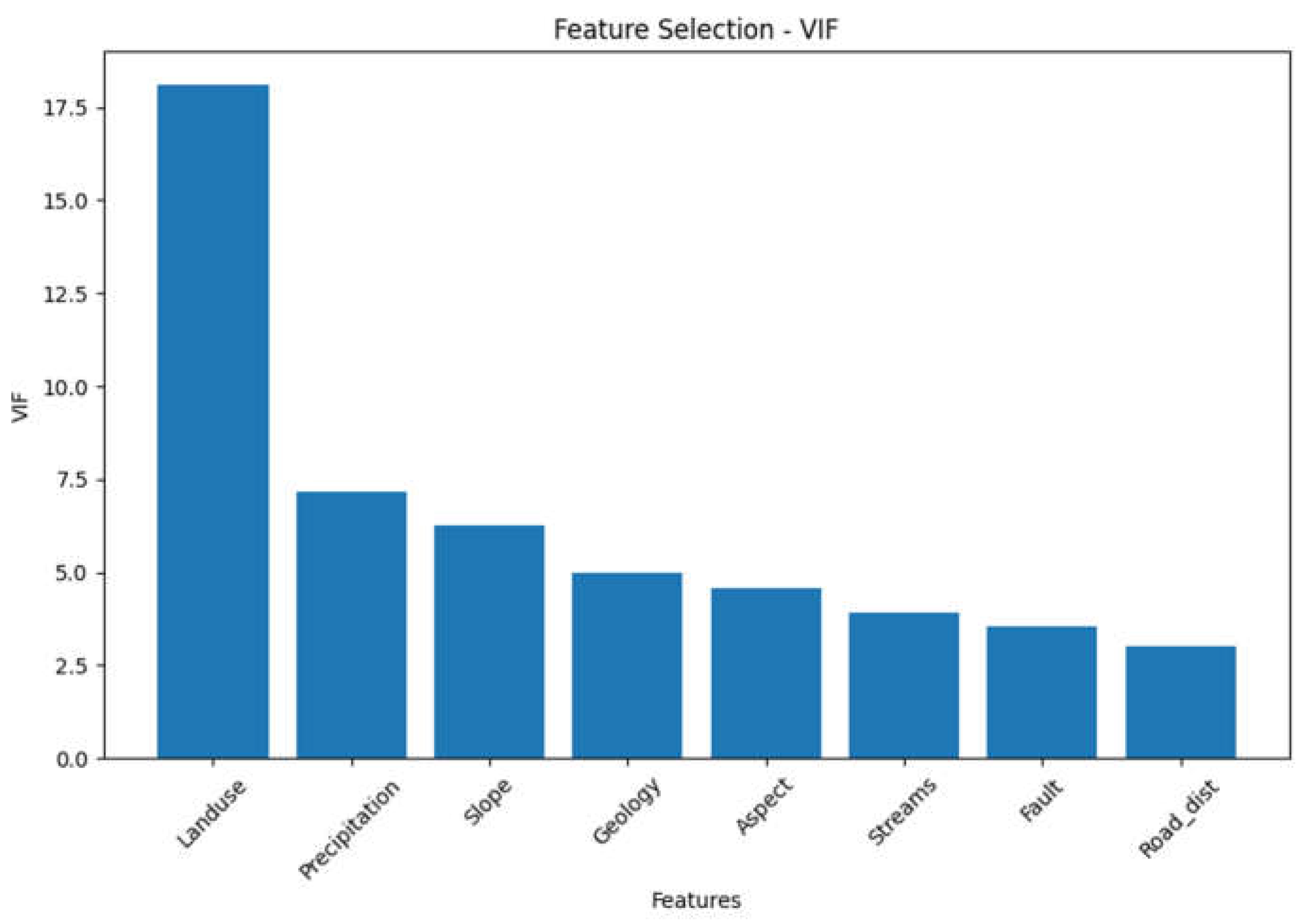
The VIF value ranges from 1 upwards, with values greater than 1 indicating the presence of multicollinearity. A VIF value of 1 indicates no multicollinearity, while values greater than 1 suggest increasing levels of multicollinearity. Generally, a VIF value of 5 or higher is often used as a threshold to identify problematic levels of multicollinearity, although the specific threshold may vary depending on the context and the field of study.

In practice, high VIF values indicate that the variance of the regression coefficient estimates for the predictor variable is inflated, which can lead to unstable and unreliable results. Multicollinearity can make it challenging to interpret the individual contributions and effects of predictor variables in the regression model. Remedial actions, such as excluding highly correlated variables or performing dimensionality reduction techniques, may be necessary to mitigate the issues caused by multicollinearity.

Table 4. Variable inflation factor VIF obtained for the geospatial variables.

Feature	VIF
Landuse	18.090383
Precipitation	7.166982
Slope	6.275566
Geology	4.986225
Aspect	4.584897
Streams	3.909876
Fault	3.531981
Road_dist	2.992487

Figure 3. Variable inflation factor VIF obtained for the geospatial variables.

3. OneR Classifier

The OneR algorithm is a simple and interpretable classification algorithm. It generates a single rule for each predictor (attribute) in the data and selects the rule with the smallest total error. Each rule is based on the value of a single attribute and predicts the most frequent class for that attribute value. The OneR classifier provides a straightforward way to assess the predictive power of individual attributes.

The OneR classifier generates a single rule for each predictor (attribute) in the data. The rule with the smallest total error is selected. The total error is calculated by summing the errors made by the rule for each attribute value. The formula for calculating the total error in OneR classifier is dependent on the evaluation metric chosen, such as misclassification error rate, accuracy, or other relevant metrics.

OneR Algorithm

For each predictor,

For each value of that predictor, make a rule as follows;

Count how often each value of target (class) appears

Find the most frequent class

Make the rule assign that class to this value of the predictor

Calculate the total error of the rules of each predictor

Choose the predictor with the smallest total error.

Table 5. Feature Accuracy score obtained for the geospatial variables using OneR classifier.

Feature Scores -OneR classifier
Feature	Accuracy Score
Road_dist	0.902439
Fault	0.707317
Streams	0.658537
Landuse	0.621951
Aspect	0.585366
Geology	0.560976
Slope	0.548780
Precipitation	0.500000
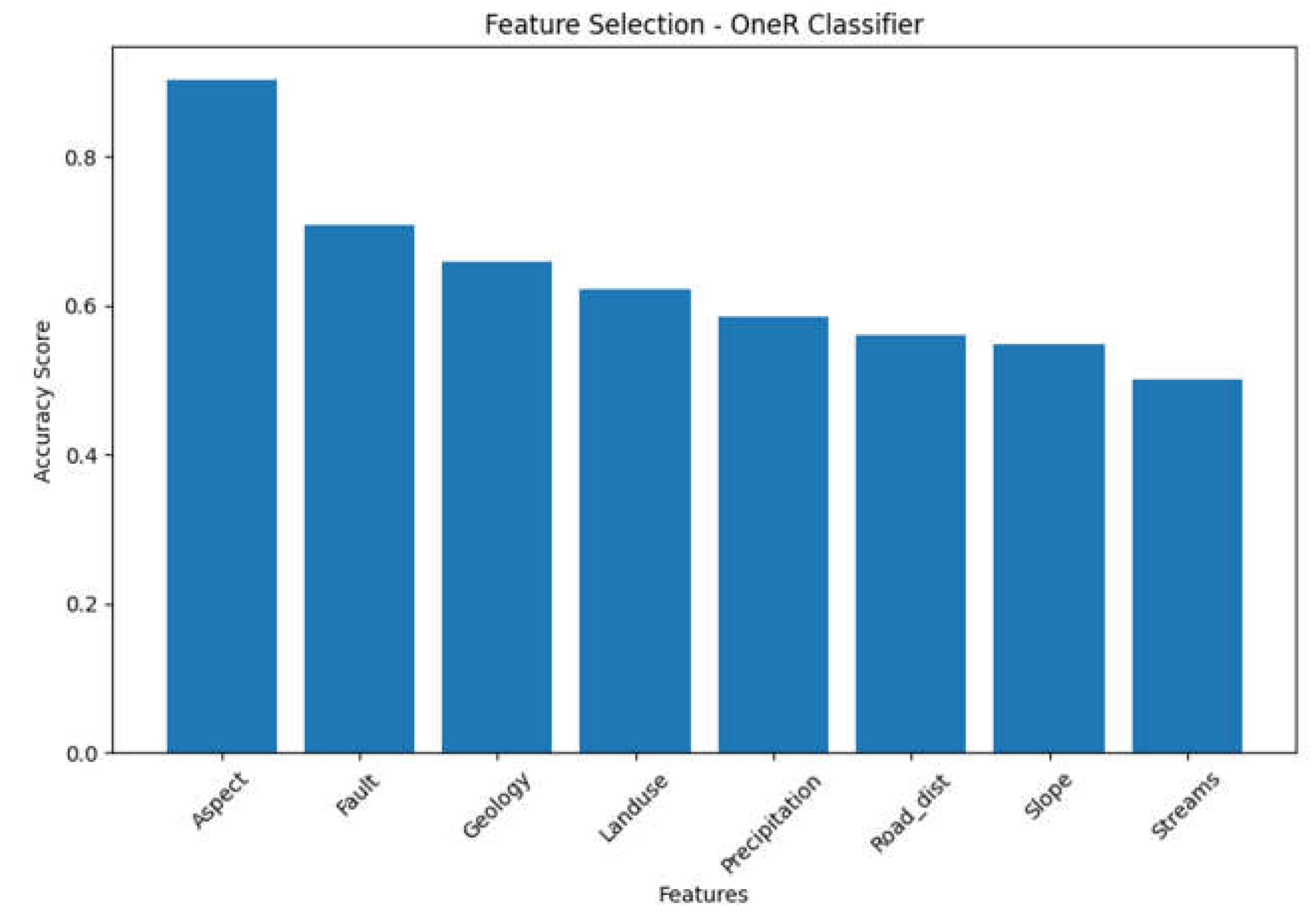
Selected Feature: Road_dist Accuracy Score: 0.902439024390

Figure 4. Feature Accuracy score obtained for the geospatial variables using OneR classifier.

4. Subset Evaluators

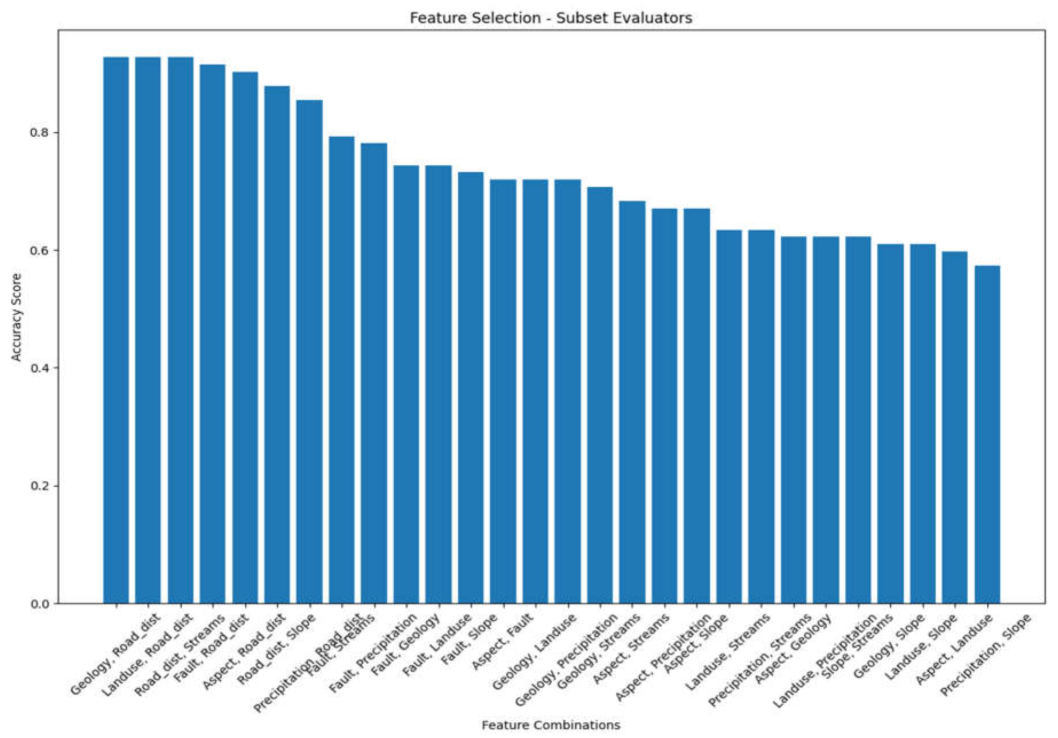
Subset evaluators evaluate the performance of feature subsets by training a classifier on either the entire training dataset or a separate hold-out testing set. They assess the accuracy or other performance metrics of different subsets to determine the most informative features. Common subset evaluators include the evaluation of classification accuracy, F1 score, or other relevant metrics to measure the effectiveness of feature subsets.

Subset evaluators assess the performance of feature subsets by training a classifier on either the entire training dataset or a separate hold-out testing set. The evaluation metric used can vary depending on the task. For example, if classification accuracy is used, the formula for calculating accuracy is:

Accuracy = (Number of correctly classified instances) / (Total number of instances)

Table 6. Feature combination accuracy score obtained for geospatial variables using subset evaluator.

Feature Combination	Accuracy Score
Geology, Road_dist	0.926829
Landuse, Road_dist	0.926829
Road_dist, Streams	0.926829
Fault, Road_dist	0.914634
Aspect, Road_dist	0.902439
Road_dist, Slope	0.878049
Precipitation,Road_dist	0.853659
Fault, Streams	0.792683
Fault, Precipitation	0.780488
Fault, Geology	0.743902
Fault, Landuse	0.743902
Fault, Slope	0.731707
Aspect, Fault	0.719512
Geology, Landuse	0.719512
Geology, Precipitation	0.719512
Geology, Streams	0.707317
Aspect, Streams	0.682927
Aspect, Precipitation	0.670732
Aspect, Slope	0.670732
Landuse, Streams	0.634146
Precipitation, Streams	0.634146
Aspect, Geology	0.621951
Landuse, Precipitation	0.621951
Slope, Streams	0.621951
Geology, Slope	0.609756
Landuse, Slope	0.609756
Aspect, Landuse	0.597561
Precipitation, Slope	0.573171

Figure 5. Feature combination accuracy score obtained for geospatial variables using subset evaluator.

5. Principal Components

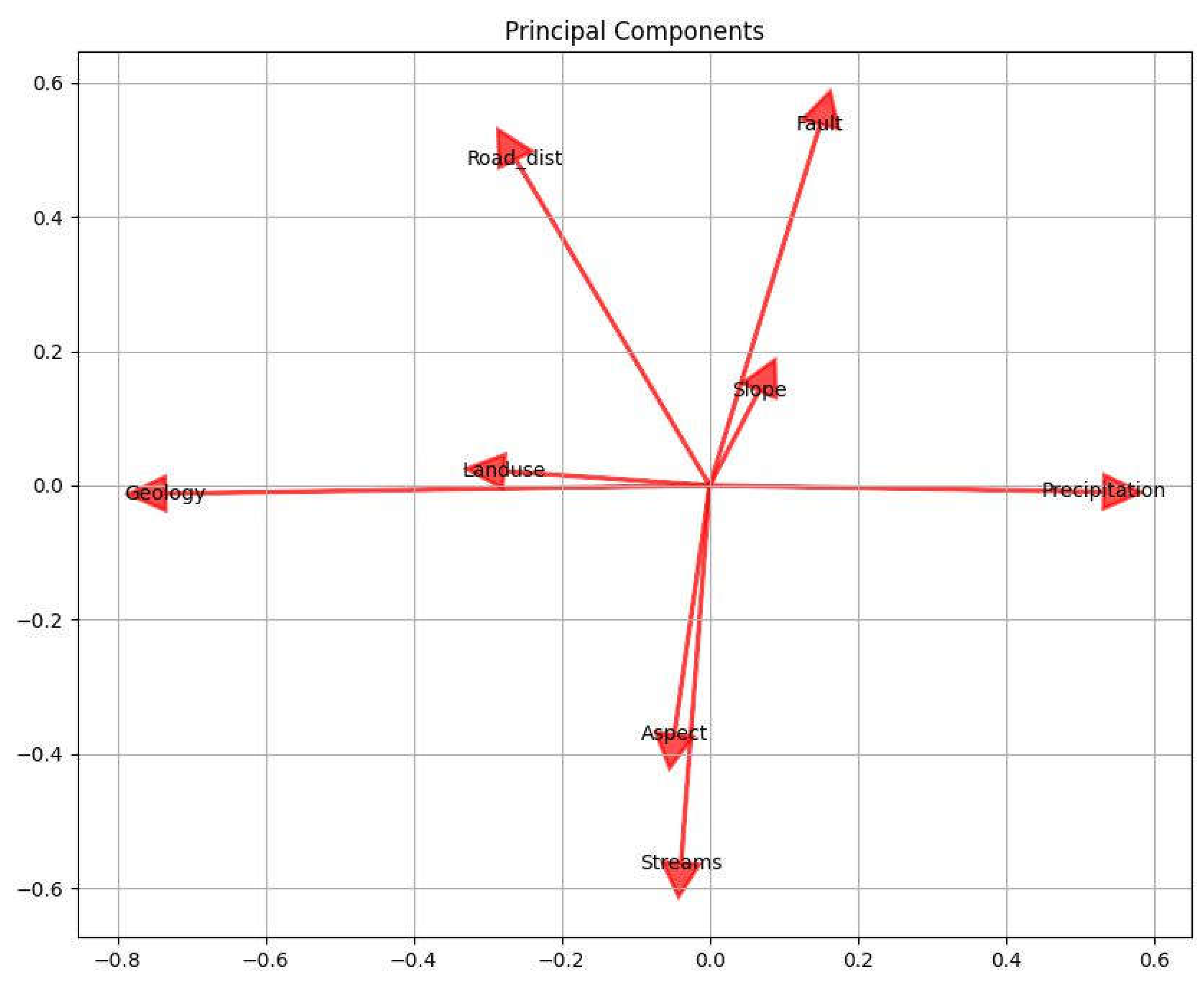
Principal Components Analysis (PCA) is a dimensionality reduction technique that transforms the original features into a new set of uncorrelated variables called principal components. These components are ordered based on the amount of variance they explain in the data. PCA helps identify the most important features by considering those associated with the highest-variance principal components, thereby reducing the dimensionality of the dataset.

Principal Components Analysis (PCA) is a mathematical technique that performs a linear transformation to convert the original correlated features into a new set of uncorrelated variables called principal components. The principal components are ordered based on the amount of variance they explain in the data. The transformation is achieved through eigendecomposition or singular value decomposition. The formulas for PCA involve eigenvalues, eigenvectors, and matrix operations.

Table 7. Principal Component Analysis (PCA) for geospatial variables used in our experiment.

Components	Variance Ratio
Aspect	27.22%
Fault	18.17%
Geology	13.66%
Land Cover	12.50%
Precipitation	10.57%
Road	9.70%
Slope	4.71%
Streams	3.48%

Figure 6. The covariance matrix is computed to understand the relationships between the features in the dataset. It represents how each feature changes with respect to the others.

6. Relief Attribute Evaluator

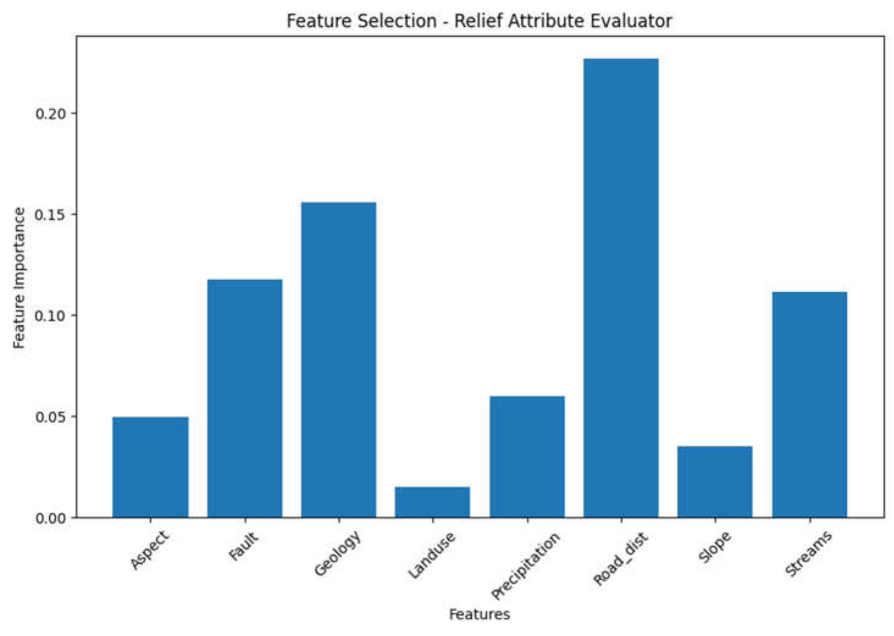
The Relief algorithm evaluates the worth of an attribute by sampling instances and comparing the attribute values of the nearest instances from the same and different classes. It measures the attribute's ability to distinguish between classes based on the differences in attribute values for nearby instances. Relief attribute evaluator is commonly used in feature selection for classification tasks, particularly for handling imbalanced datasets.

The Relief algorithm evaluates the worth of an attribute by sampling instances and comparing the attribute values of the nearest instances from the same and different classes. Relief computes the weight for each attribute based on the differences in attribute values between the nearest instances. The formula for the weight calculation in Relief is:

Weight(i) = sum(NearHit(i)) / k - sum(NearMiss(i)) / k

where:

Weight(i) is the weight assigned to the attribute i.

NearHit(i) represents the differences in attribute values between the nearest instances of the same class.

NearMiss(i) represents the differences in attribute values between the nearest instances of different classes.

k is the number of nearest neighbors considered.

Table 8. Geospatail variable importence obtained from Relief Attribute Evaluator.

Feature	Importance
Road_dist	0.226967
Geology	0.155882
Fault	0.117683
Streams	0.111745
Precipitation	0.059804
Aspect	0.049510
Slope	0.035294
Landuse	0.015196

Figure 7. Geospatail variable importence obtained from Relief Attribute Evaluator.

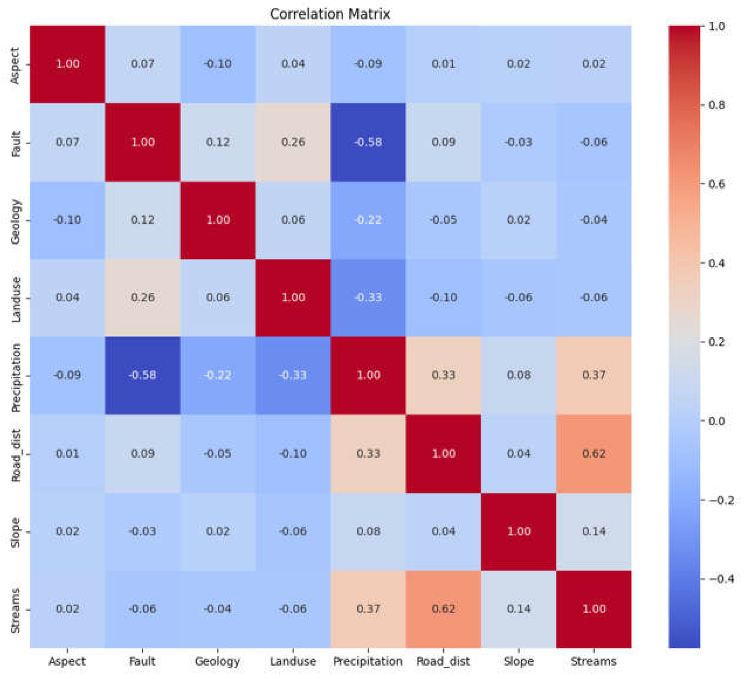
7. Correlation

Correlation measures the linear relationship between an attribute and the class variable. Pearson's correlation coefficient is a common measure used to assess the strength and direction of the linear association. Higher absolute correlation values indicate a stronger relationship between the attribute and the class variable. Correlation analysis helps identify attributes that exhibit a significant relationship with the target variable.

Correlation measures the linear relationship between an attribute and the class variable. Pearson's correlation coefficient is commonly used to assess the strength and direction of the linear association. The formula for Pearson's correlation coefficient is:

Correlation = Cov(X, Y) / (StdDev(X) * StdDev(Y))

where:

Cov(X, Y) is the covariance between the attribute X and the class variable Y.

StdDev(X) is the standard deviation of attribute X.

StdDev(Y) is the standard deviation of the class variable Y.

Table 9. Geospatail variable importence obtained from Correlation.

Feature	Importance
Aspect	1.000000
Geology	0.099800
Precipitation	0.089989
Fault	0.065930
Landuse	0.042576
Streams	0.022152
Slope	0.019784
Road_dist	0.005355

Figure 8. Geospatail variable importance obtained from Correlation.

8. Symmetrical Uncertainty

Symmetrical Uncertainty is an information-theoretic correlation measure based on entropy. It quantifies the amount of shared information between an attribute and the class variable. The measure takes into account both the attribute's predictability of the class and the class's predictability of the attribute. Symmetrical Uncertainty allows for assessing the mutual dependence between attributes and the target variable, enabling the identification of informative attributes.

Symmetrical Uncertainty = (2 * Mutual Information) / (Entropy(X) + Entropy(Y))

where:

Mutual Information measures the amount of shared information between the attribute X and the class variable Y.

Entropy(X) is the entropy of attribute X.

Entropy(Y) is the entropy of the class variable Y.

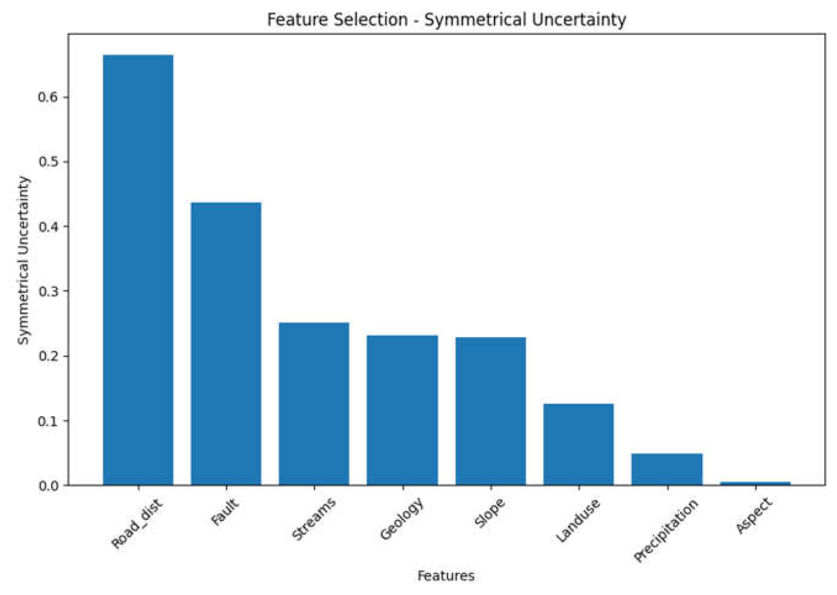
Each of these feature selection techniques offers a unique approach to assess the importance and relevance of geospatial variables for landslide susceptibility mapping. They provide different perspectives and criteria to evaluate the impact of variables on the target variable, allowing researchers and practitioners to gain valuable insights into the most influential factors affecting landslide occurrences along the Karakoram Highway.

Table 10. Symmetrical Uncertainty obtained for the Geospatail variables.

Feature	Symmetrical Uncertainty
Road_dist	0.663892
Fault	0.435661
Streams	0.251117
Geology	0.231301
Slope	0.227836
Landuse	0.126103
Precipitation	0.048381
Aspect	0.005321

Figure 9. Symmetrical Uncertainty obtained for the Geospatail variables.

In conclusion, after analyzing the eight different techniques , we can observe a consistent presence of the feature "Road_dist" in all of them. "Road_dist" demonstrates several favorable characteristics across the tables, including high information gain, low multicollinearity as indicated by a low VIF, high accuracy scores in the OneR classifier, inclusion in high-accuracy feature combinations, and relatively high importance scores in the Relief Attribute Evaluator and Symmetrical Uncertainty.

These findings suggest that "Road_dist" holds potential significance and influence in the analysis, regardless of the specific evaluation technique or metric employed.Additionally, the tables provide further insights into other features. For example, "Fault" and "Streams" show relatively high information gain, "Aspect" has a high variance ratio in the PCA components, and "Aspect" and "Slope" display lower importance scores and correlations with the target variable.

It is important to consider the specific evaluation techniques and measures employed in each table when interpreting the results. The presence of "Road_dist" consistently throughout the tables suggests that it should be considered for inclusion in the feature set for the landslide susceptibility mapping task. However, to make a final determination, it is recommended to conduct a comprehensive analysis, including assessing multicollinearity, evaluating the contributions of other features, and considering additional factors such as interpretability and practicality. Such analysis will help determine the optimal set of variables for accurate and reliable landslide susceptibility mapping.

Benefits of artificial neural networks

Artificial neural networks (ANNs) offer several benefits in various fields and applications. Here are some of the key benefits of using ANNs. Nonlinear mapping , ANNs excel at capturing and modeling complex, nonlinear relationships between input and output variables. They can learn and represent highly intricate patterns, making them effective in handling complex tasks that may not have clear linear relationships. Adaptive learning, ANNs have the ability to adapt and learn from examples or data. Through a process called training, ANNs can adjust their internal parameters to improve their performance on specific tasks. This adaptability allows ANNs to continuously learn and improve their predictions or classifications as new data becomes available. Parallel Processing, ANNs can perform computations in parallel, making them suitable for handling large-scale and computationally intensive tasks [29-31]. This parallel processing capability enables ANNs to process multiple inputs simultaneously, leading to faster and more efficient computations. Fault Tolerance and Redundancy, ANNs have the ability to tolerate faults or errors in the system. Due to their distributed nature and interconnected structure, ANNs can still provide useful outputs even when some of the nodes or connections in the network are damaged or missing. This fault tolerance and redundancy make ANNs robust in real-world scenarios where there may be noise or incomplete data. Pattern Recognition and Classification, ANNs are highly effective in pattern recognition and classification tasks [32-35]. They can learn and recognize complex patterns, allowing them to classify and categorize data into different classes or groups. This capability has numerous applications in fields such as image and speech recognition, natural language processing, and data mining. Generalization, ANNs can generalize learned patterns to new, unseen data. Once trained on a representative dataset, ANNs can make accurate predictions or classifications on similar but previously unseen inputs. This generalization ability makes ANNs valuable in scenarios where new data needs to be processed or classified in real-time. Feature Extraction, ANNs can automatically extract relevant features or representations from raw data, reducing the need for manual feature engineering. This capability is particularly useful when dealing with high-dimensional data, as ANNs can automatically learn and extract the most informative features to improve performance. Real-Time Processing, ANNs can be implemented in real-time systems, allowing for quick and efficient processing of data. This capability is crucial in applications such as real-time monitoring, control systems, and decision-making where immediate responses are required. These benefits demonstrate the versatility and power of artificial neural networks in solving complex problems and making accurate predictions or classifications across various domains.

3. Metaheuristic and Bayesian algorithms

Genetic algorithms

Although it is difficult to guarantee that the ANN can always generalize the testing data successfully, using a genetic method to avoid the model from getting stuck in a local minimum situation could assist increase accuracy rates. The three main components of the genetic algorithm (GA) are crossover, mutation, and selection. To realize elitism, the process first chooses the elite parents for the gene pool (a list that monitors the best weighting matrix). The crossover is then put into practice. The method chooses two genes at random from the best genes (weighted matrix) and recombines them according to a specific strategy specified in the accompanying Python code. For instance, I chose a split point for the elite genes 1 and 2 at random in this instance. I then combine the second portion of gene 2 with the first part of gene 1, and for the remaining pieces of the two genes, I do the reverse procedure. I have two possibly elite genes that were recombined as a result. Third, given that it occurs at random, a mutation could happen. After completing the crossover for each generation, the mechanism will produce a random integer between 0 and 1. A specific area of the weighted matrix, which is likewise created randomly, will be multiplied by yet another random number between 2 and 5 if the randomly generated value is less than or equal to 0.05. To facilitate the mutation process and avoid the ANN model from being trained in the wrong direction (resulting in a poorer training accuracy rate), some weighted matrix values can be slightly scaled. An ANN's performance could be impacted by a wide range of variables. The number of layers, the number of neurons in each layer, the learning rate, the optimization function, the loss function, and other factors are among them [36-40]. In a genetic algorithm, the ANN must be constructed while taking into account the population size, number of generations, crossover rate, mutation rate, and probability. The model should provide a weighted matrix with a higher variance of values than those with a lower mutation rate and lower mutation probability, for example, if the mutation rate and its mutation probability are high. Its major objective is to attempt to address the flaw in the conventional gradient descent learning technique by ensuring that there are a variety of feasible weighted matrices rather than maybe training a model in the incorrect manner without obtaining the best possible solution for any problem.

PSO

PSO, which stands for Particle Swarm Optimization, is a metaheuristic optimization algorithm inspired by the behavior of bird flocking or fish schooling. It is commonly used in combination with artificial neural networks (ANNs) to optimize their performance. In the context of ANNs, PSO is employed to determine the optimal values of the ANN's parameters or weights. The algorithm operates by simulating a population of particles that move through a multidimensional search space. Each particle represents a potential solution or set of parameters for the ANN.

Initially, the particles are assigned random positions and velocities within the search space. The positions represent the values of the ANN's parameters, while the velocities determine the particles' movement direction and speed. The algorithm then evaluates the fitness or performance of each particle's solution by training the ANN with the corresponding parameter values and measuring its accuracy or error. During each iteration of the algorithm, the particles adjust their velocities and positions based on their own historical best solution (the best fitness achieved by the particle itself) and the global best solution (the best fitness achieved by any particle in the swarm). This collective learning and sharing of information guide the particles towards promising regions in the search space.

The adjustment of particle velocities is governed by two main factors: cognitive component and social component. The cognitive component represents the particle's own knowledge and encourages it to move towards its best solution. The social component reflects the influence of the swarm and directs the particle towards the global best solution. As the iterations progress, the particles converge towards the optimal parameter values, which correspond to the weights that result in the best performance of the ANN. The algorithm terminates when a specified stopping criterion is met, such as reaching a maximum number of iterations or achieving a desired level of performance [5,41-44]. By using PSO, ANN models can be effectively fine-tuned and optimized to improve their accuracy, convergence speed, and generalization capabilities. PSO provides a powerful approach for exploring and exploiting the parameter space of ANNs, leading to enhanced performance in a variety of tasks and applications.

BO-GP

Bayesian optimization with Gaussian process (BO-GP) is a metaheuristic optimization algorithm commonly used for fine-tuning and optimizing artificial neural network (ANN) models. It combines Bayesian optimization, which is a sequential model-based optimization approach, with Gaussian processes, which are statistical models used for modeling the behavior of functions. In the context of ANN models, BO-GP aims to find the optimal set of hyperparameters that result in the best performance for the given task [45-47]. These hyperparameters include the number of hidden layers, the number of neurons in each layer, the learning rate, regularization parameters, activation functions, and other architectural choices. The BO-GP algorithm works iteratively as follows:

Define a search space: Determine the range or values for each hyperparameter that will be explored during the optimization process.
Create an initial design: Select a small set of initial hyperparameter configurations to evaluate the ANN model's performance. This initial design is often chosen using techniques like random sampling.
Build a surrogate model: Fit a Gaussian process regression model to the initial design data. The surrogate model approximates the behavior of the ANN model based on the observed hyperparameter-performance pairs.
Optimize the acquisition function: The acquisition function guides the selection of the next set of hyperparameters to evaluate. It balances exploration (sampling new regions of the search space) and exploitation (focusing on promising regions). Common acquisition functions include Expected Improvement (EI), Upper Confidence Bound (UCB), and Probability of Improvement (PI).
Evaluate the ANN model: Select the next set of hyperparameters based on the optimized acquisition function and evaluate the performance of the ANN model with those hyperparameters. This involves training the ANN on a training set and evaluating its performance on a validation set or using cross-validation.
Update the surrogate model: Incorporate the new hyperparameter-performance pair into the existing data and update the Gaussian process regression model. This allows the surrogate model to improve its approximation of the ANN model's behavior.
Repeat steps 4 to 6: Iterate the process by optimizing the acquisition function, evaluating the ANN model, and updating the surrogate model until reaching a specified termination criterion (e.g., a maximum number of iterations or a desired level of performance).

The goal of BO-GP is to efficiently explore the hyperparameter search space and find the optimal configuration that maximizes the performance of the ANN model. By leveraging Bayesian optimization and Gaussian process modeling, BO-GP balances exploration and exploitation, enabling effective hyperparameter tuning and improving the overall performance of ANN models.

BO-TPE

(Bayesian Optimization with Tree-structured Parzen Estimator) is another metaheuristic optimization algorithm commonly used for fine-tuning and optimizing artificial neural network (ANN) models. It is a variant of Bayesian optimization that employs a Tree-structured Parzen Estimator to model the performance of different hyperparameter configurations.

The BO-TPE algorithm works in the following steps:

Define a search space: Specify the range or values for each hyperparameter that will be explored during the optimization process.
Initialize the hyperparameter sampling: Randomly sample a set of hyperparameter configurations from the search space to create an initial design.
Evaluate the initial design: Train and evaluate the ANN models corresponding to the initial set of hyperparameter configurations. This typically involves splitting the data into training and validation sets and using cross-validation or hold-out validation.
Build a probabilistic model: Based on the observed hyperparameter-performance pairs from the initial design, construct a probabilistic model using a Tree-structured Parzen Estimator. This model captures the relationship between hyperparameter values and the corresponding performance of the ANN models.
Update the model and sample new hyperparameters: The Tree-structured Parzen Estimator uses the previous observations and probabilistic model to guide the sampling of new hyperparameters for the next iteration. It balances exploration (sampling new regions) and exploitation (focusing on promising regions) by considering both the probability of improvement and the expected improvement.
Evaluate the new hyperparameter configurations: Train and evaluate the ANN models with the newly sampled hyperparameter configurations. Update the observed hyperparameter-performance pairs.
Update the probabilistic model: Incorporate the new observations into the probabilistic model. This allows the model to refine its estimation of the performance landscape and guide the sampling process more effectively.
Repeat steps 5 to 7: Iterate the process by sampling new hyperparameters, evaluating the ANN models, and updating the probabilistic model until reaching a termination criterion, such as a maximum number of iterations or a desired level of performance.

BO-TPE leverages the Bayesian optimization framework to efficiently explore the hyperparameter search space and identify the optimal configuration for the ANN model. By using a Tree-structured Parzen Estimator, it captures the complex relationship between hyperparameters and performance, enabling effective hyperparameter tuning and improving the overall performance of ANN models [48-50].

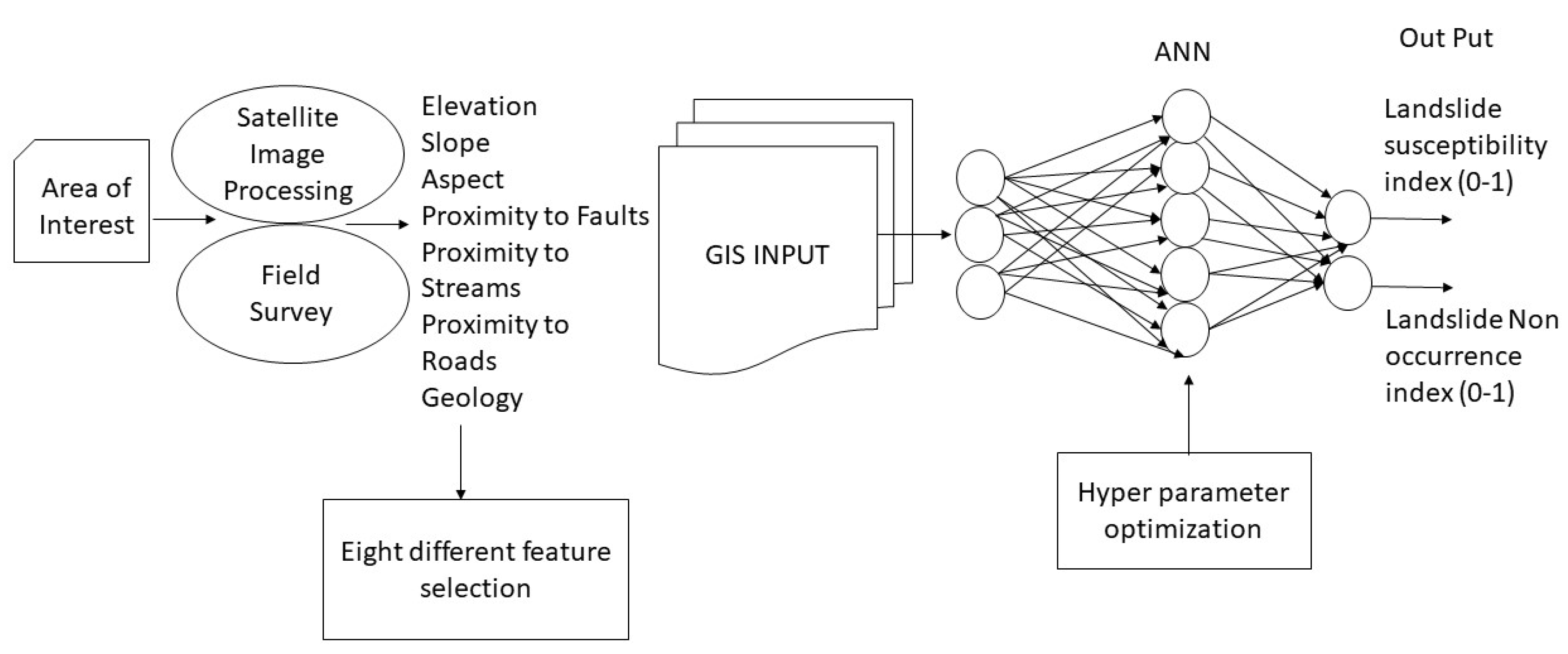
4. Methodology

The study employed HOP techniques to search for the optimal hyperparameter configurations for the ANN models. This is important because selecting appropriate hyperparameters, such as activation function, batch size, epochs, and neuron configurations, can significantly impact the performance and generalization capabilities of ANNs. The four optimization techniques used in the study, namely PSO, GA, BO_GP, and BO_TPE, were applied to fine-tune the hyperparameters of the ANN models. Each technique employs a different approach to explore the hyperparameter space and find the best set of values. The performance of the ANN models was evaluated using area under the ROC curve (AUROC). We also used eight different feature selection techniques to analyze the importance of geospatial variables through different feature selection techniques. Overall, the methodology involved applying different optimization and feature selection techniques to search for the optimal hyperparameter and input feature configurations for the ANN models. The methodology aims to identify the most effective feature selection and optimization approach and hyperparameter and input feature settings for accurately predicting the landslide susceptibility index.

Figure 10. Methodology used for our experiment.

5. Results

Using the Keras model in Python, I evaluated ANN models trained using Adam (Adaptive Moment Estimation). The outputs of the various algorithms are shown below. It is evident from our results that both bayesian optimization and metaheuristic algorithms, such as particle swarm optimization (PSO) and genetic algorithm (GA), can both be effective for optimizing artificial neural networks (ANNs) due to their complementary strengths and capabilities. Here are some reasons why Bayesian optimization and metaheuristic algorithms can perform equally well for ANN optimization. Bayesian optimization is known for its ability to balance exploitation (exploiting known good solutions) and exploration (exploring new regions in the search space). It uses probabilistic models to guide the search towards promising regions, based on observed performance. On the other hand, metaheuristic algorithms like PSO and GA incorporate stochastic search techniques that can explore the search space more extensively, searching for global optima. ANNs often have a large number of hyperparameters, making the optimization problem high-dimensional. Bayesian optimization excels in handling high-dimensional spaces by building surrogate models that capture the relationship between hyperparameters and performance. It effectively guides the search to promising regions based on the surrogate model's predictions. Metaheuristic algorithms can also handle high-dimensional spaces through their population-based search, which allows for more diverse exploration.

The performance landscape of ANNs can be complex and non-convex, with multiple local optima. Bayesian optimization and metaheuristic algorithms approach the optimization problem from different perspectives. Bayesian optimization focuses on modeling the performance landscape and exploiting its information to guide the search, while metaheuristic algorithms explore the landscape through heuristics and search operators to escape local optima. Both Bayesian optimization and metaheuristic algorithms offer flexibility in terms of the search strategy and problem representation. They can be applied to different types of optimization problems, including ANN optimization, by adapting their operators or objective functions accordingly. This adaptability allows them to be tuned and customized based on the specific requirements of the ANN optimization task.

Ultimately, the effectiveness of Bayesian optimization and metaheuristic algorithms for ANN optimization can depend on various factors, including the problem complexity, the size of the search space, and the availability of computational resources. It is often beneficial to experiment with different optimization techniques and select the one that performs best for a particular ANN optimization task.

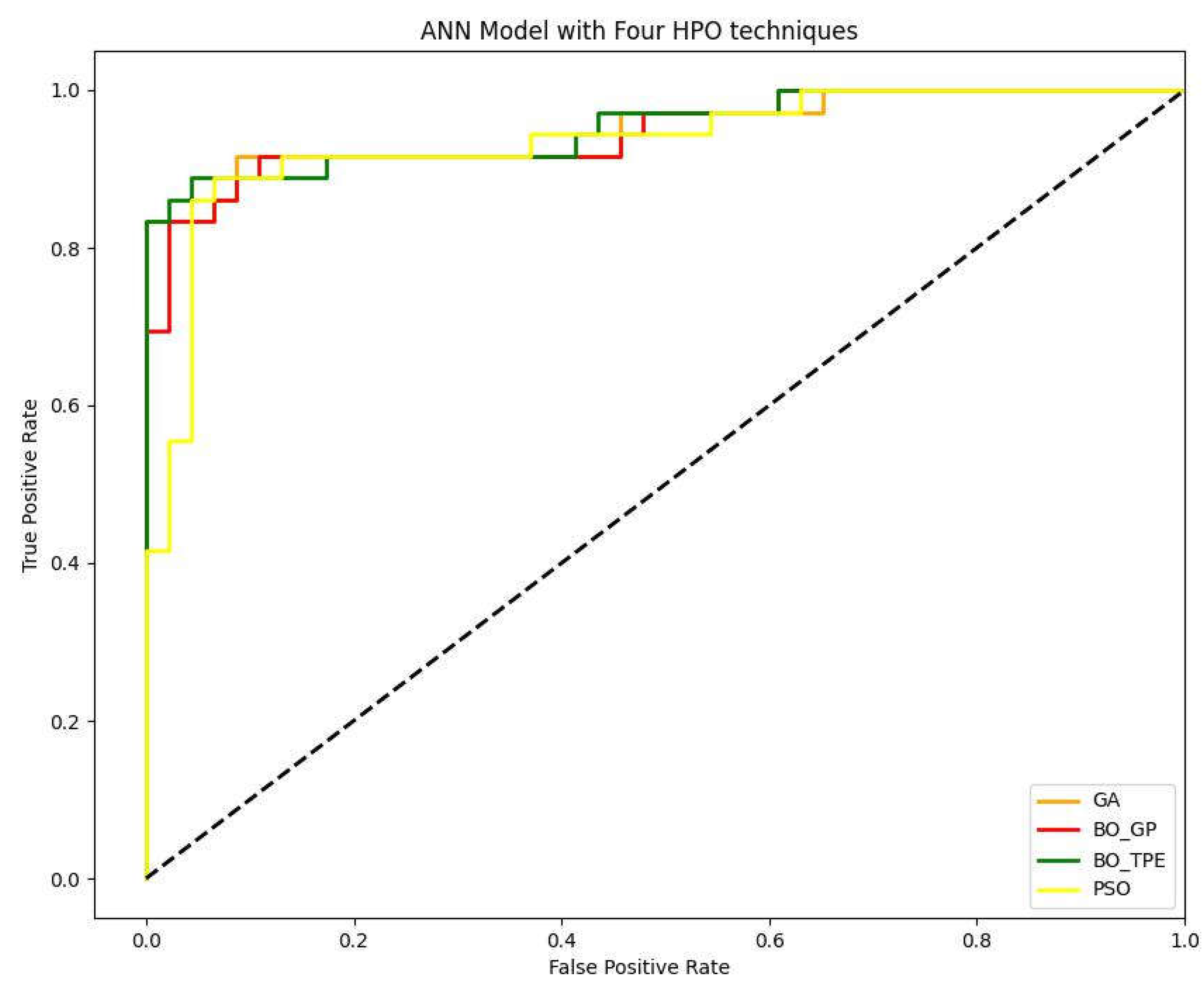
Figure 11. AUC value for GA, BO_GP, BO_TPE and PSO for ANN model.

The results of the AUC values indicate the performance of each HPO technique in optimizing the hyperparameters of the ANN for the given ML task. A higher AUC value generally indicates better discrimination power and predictive accuracy of the model.

Based on the given data, BO_TPE achieved the highest AUC value of 0.95289, followed by GA with 0.94987, BO_GP with 0.94685, and PSO with 0.93538. This suggests that BO_TPE performed the best among the evaluated HPO techniques for the given ML task.

There could be several reasons why BO_TPE outperformed the other techniques. BO_TPE combines both exploration and exploitation strategies effectively. It intelligently explores the hyperparameter space to identify promising regions and then exploits the information gained to refine the search for optimal hyperparameters. This balance between exploration and exploitation can lead to better performance. BO_TPE utilizes a sequential Bayesian optimization strategy, which leverages the information gathered from previous iterations to guide the search for optimal hyperparameters. This adaptive approach helps in efficiently exploring the hyperparameter space and quickly converging to promising solutions. BO_TPE employs a tree-structured Parzen estimator (TPE) to efficiently explore the hyperparameter space. TPE focuses more on areas that are likely to contain better hyperparameter configurations, allowing for more efficient optimization compared to other techniques. BO_TPE utilizes the observed performance of previous hyperparameter configurations to build a probabilistic model and guide the search towards regions with higher potential. This exploitation of information helps in quickly identifying and refining good hyperparameter settings.

It's important to note that the performance of HPO techniques can vary depending on the specific dataset, ML task, and hyperparameter space being considered. The given results suggest that, for the specific ML task and dataset, BO_TPE performed better than GA, BO_GP, and PSO in optimizing the hyperparameters of the ANN model, resulting in higher predictive accuracy and discrimination power as indicated by the AUC values.

Table 11. AUC value for GA, BO_GP, BO_TPE and PSO for ANN model.

HPO Techniques	ML	AUC
GA	ANN	0.94987
BO_GP	ANN	0.94685
BO_TPE	ANN	0.95289
PSO	ANN	0.93538

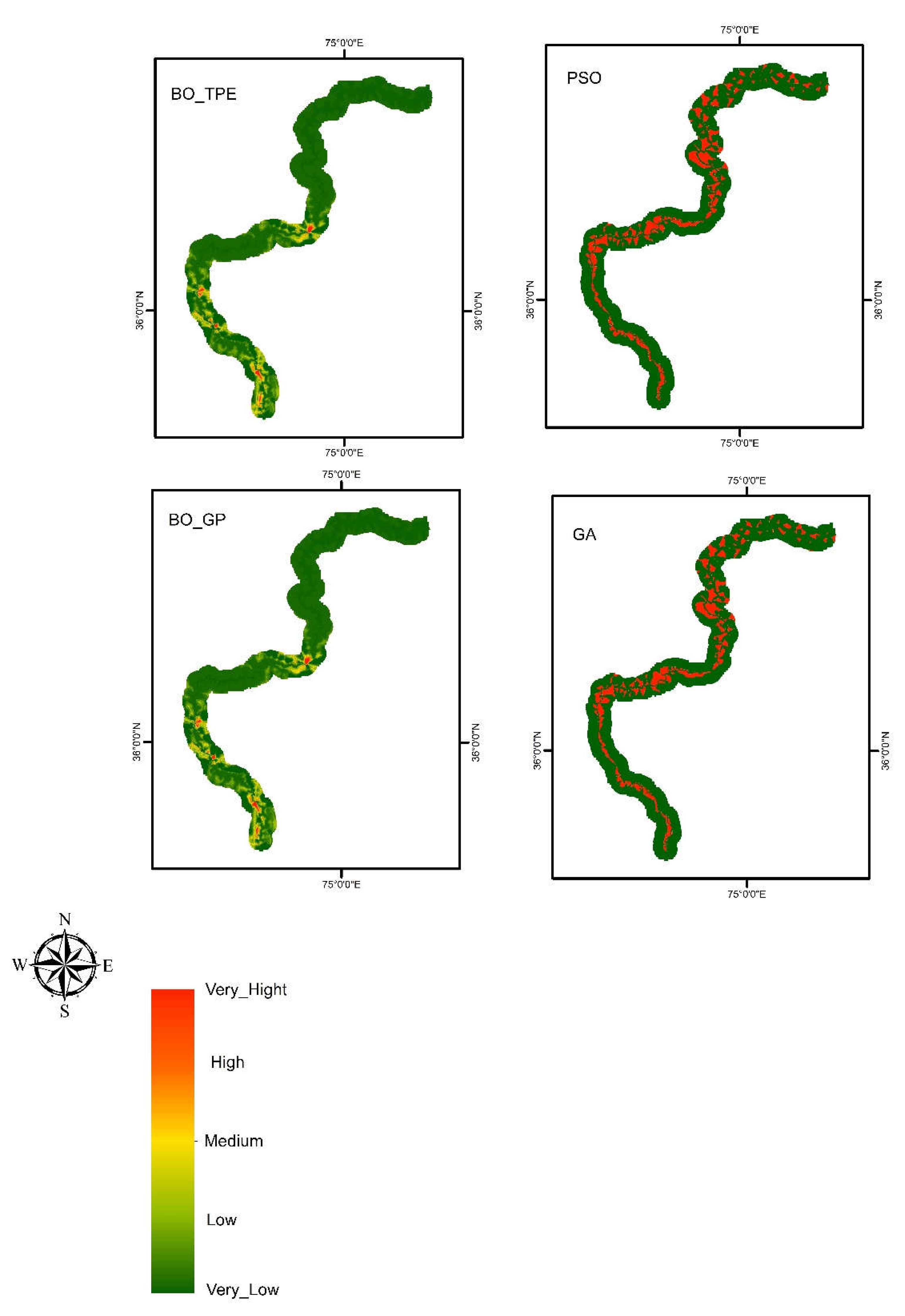
Figure 12. The landslide susceptibility maps generated by ANN using different optimization techniques such as BO_TPE, BO_GP, PSO and GA.

Funding

We extend our appreciation to the Researchers Supporting Project (no. RSP2023R218), King Saud University, Riyadh, Saudi Arabia.

Data Availability Statement

The data presented in the study are available on request from the first and corresponding author. The data are not publicly available due to the thesis that is being prepared from these data.

Conflicts of Interest

The authors declare no conflict of interest.

References

Hagan, M.; Demuth, H.; Beale, M. Neural network design (PWS, Boston, MA). Google Scholar Google Scholar Digital Library Digital Library 1996. [Google Scholar]
Werbos, P.J. Backpropagation through time: what it does and how to do it. Proceedings of the IEEE 1990, 78, 1550–1560. [Google Scholar] [CrossRef]
Hertz, J.; Krogh, A.; Palmer, R.G.; Horner, H. Introduction to the theory of neural computation. Physics Today 1991, 44, 70. [Google Scholar] [CrossRef]
Hagan, M.T.; Menhaj, M.B. Training feedforward networks with the Marquardt algorithm. IEEE transactions on Neural Networks 1994, 5, 989–993. [Google Scholar] [CrossRef]
Moayedi, H.; Mehrabi, M.; Mosallanezhad, M.; Rashid, A.S.A.; Pradhan, B. Modification of landslide susceptibility mapping using optimized PSO-ANN technique. Engineering with Computers 2019, 35, 967–984. [Google Scholar] [CrossRef]
Gianola, D.; Okut, H.; Weigel, K.A.; Rosa, G.J. Predicting complex quantitative traits with Bayesian neural networks: a case study with Jersey cows and wheat. BMC genetics 2011, 12, 1–14. [Google Scholar] [CrossRef]
Bao, Y.; Velni, J.M.; Shahbakhti, M. Epistemic uncertainty quantification in state-space LPV model identification using Bayesian neural networks. IEEE control systems letters 2020, 5, 719–724. [Google Scholar] [CrossRef]
Sultana, N.; Hossain, S.Z.; Abusaad, M.; Alanbar, N.; Senan, Y.; Razzak, S. Prediction of biodiesel production from microalgal oil using Bayesian optimization algorithm-based machine learning approaches. Fuel 2022, 309, 122184. [Google Scholar] [CrossRef]
Kolar, D.; Lisjak, D.; Pająk, M.; Gudlin, M. Intelligent fault diagnosis of rotary machinery by convolutional neural network with automatic hyper-parameters tuning using bayesian optimization. Sensors 2021, 21, 2411. [Google Scholar] [CrossRef]
Salman, I.; Ucan, O.N.; Bayat, O.; Shaker, K. Impact of metaheuristic iteration on artificial neural network structure in medical data. Processes 2018, 6, 57. [Google Scholar] [CrossRef]
Dhar, A.R.; Gupta, D.; Roy, S.S.; Lohar, A.K. Forward and backward modeling of direct metal deposition using metaheuristic algorithms tuned artificial neural network and extreme gradient boost. Progress in Additive Manufacturing 2022, 1–15. [Google Scholar] [CrossRef]
Zhao, Y.; Hu, H.; Song, C.; Wang, Z. Predicting compressive strength of manufactured-sand concrete using conventional and metaheuristic-tuned artificial neural network. Measurement 2022, 194, 110993. [Google Scholar] [CrossRef]
Mehrabi, M.; Moayedi, H. Landslide susceptibility mapping using artificial neural network tuned by metaheuristic algorithms. Environmental Earth Sciences 2021, 80, 1–20. [Google Scholar] [CrossRef]
Zhao, G.; Zhang, C.; Zheng, L. Intrusion detection using deep belief network and probabilistic neural network. In Proceedings of the 2017 IEEE international conference on computational science and engineering (CSE) and IEEE international conference on embedded and ubiquitous computing (EUC); 2017; pp. 639–642. [Google Scholar]
Karegowda, A.G.; Devika, G. Meta-heuristic parameter optimization for ANN and real-time applications of ANN. In Research Anthology on Artificial Neural Network Applications; IGI Global, 2022; pp. 166–201. [Google Scholar]
MAMINDLA, A.K.; RAMADEVI, D.; SEDOVA, O.V.; ALEKSEEV, A.G.; ASHRAF, M.T.; ARIFFIN, D.S.B.B.; SAMY, S.; FOUZIA, E.; NABIL, E.; KHALID, S. ANN-ABC META-HEURISTIC HYPER PARAMETER TUNING FOR MAMMOGRAM CLASSIFICATION. Journal of Theoretical and Applied Information Technology 2023, 101. [Google Scholar]
Shafqat, W.; Malik, S.; Lee, K.-T.; Kim, D.-H. PSO based optimized ensemble learning and feature selection approach for efficient energy forecast. Electronics 2021, 10, 2188. [Google Scholar] [CrossRef]
Elgeldawi, E.; Sayed, A.; Galal, A.R.; Zaki, A.M. Hyperparameter tuning for machine learning algorithms used for arabic sentiment analysis. In Proceedings of the Informatics; 2021; p. 79. [Google Scholar]
Maniezzo, V. Genetic evolution of the topology and weight distribution of neural networks. IEEE Transactions on neural networks 1994, 5, 39–53. [Google Scholar] [CrossRef]
Fischer, M.M.; Leung, Y. A genetic-algorithms based evolutionary computational neural network for modelling spatial interaction dataNeural network for modelling spatial interaction data. The Annals of Regional Science 1998, 32, 437–458. [Google Scholar] [CrossRef]
Irani, R.; Nasimi, R. Evolving neural network using real coded genetic algorithm for permeability estimation of the reservoir. Expert Systems with Applications 2011, 38, 9862–9866. [Google Scholar] [CrossRef]
Miller, G.F.; Todd, P.M.; Hegde, S.U. Designing Neural Networks Using Genetic Algorithms. In Proceedings of the ICGA; 1989; pp. 379–384. [Google Scholar]
Liu, Z.; Liu, A.; Wang, C.; Niu, Z. Evolving neural network using real coded genetic algorithm (GA) for multispectral image classification. Future Generation Computer Systems 2004, 20, 1119–1129. [Google Scholar] [CrossRef]
Abbas, F.; Zhang, F.; Iqbal, J.; Abbas, F.; Alrefaei, A.F.; Albeshr, M. Assessing the Dimensionality Reduction of the Geospatial Dataset Using Principal Component Analysis (PCA) and Its Impact on the Accuracy and Performance of Ensembled and Non-ensembled Algorithms. Preprints.org 2023. [Google Scholar] [CrossRef]
Wong, Y.J.; Arumugasamy, S.K.; Jewaratnam, J. Performance comparison of feedforward neural network training algorithms in modeling for synthesis of polycaprolactone via biopolymerization. Clean Technologies and Environmental Policy 2018, 20, 1971–1986. [Google Scholar] [CrossRef]
Hessami, M.; Anctil, F.; Viau, A.A. Selection of an artificial neural network model for the post-calibration of weather radar rainfall estimation. Journal of Data Science 2004, 2, 107–124. [Google Scholar] [CrossRef]
Arthur, C.K.; Temeng, V.A.; Ziggah, Y.Y. Performance evaluation of training algorithms in backpropagation neural network approach to blast-induced ground vibration prediction. Ghana Mining Journal 2020, 20, 20–33. [Google Scholar] [CrossRef]
Abbas, F.; Zhang, F.; Ismail, M.x.; Khan, G.; Iqbal, J.; Alrefaei, A.F.; Albeshr, M.F. Hyperparameter Optimization for Landslide Susceptibility Mapping: A Comparison between Baseline, Bayesian and Metaheuristic Hyperparameter Optimization Techniques for Machine Learning Algorithms. Preprints.org 2023. [Google Scholar] [CrossRef]
Gardner, M.W.; Dorling, S. Artificial neural networks (the multilayer perceptron)—a review of applications in the atmospheric sciences. Atmospheric environment 1998, 32, 2627–2636. [Google Scholar] [CrossRef]
Lisboa, P.J.; Taktak, A.F. The use of artificial neural networks in decision support in cancer: a systematic review. Neural networks 2006, 19, 408–415. [Google Scholar] [CrossRef]
Lisboa, P.J. A review of evidence of health benefit from artificial neural networks in medical intervention. Neural networks 2002, 15, 11–39. [Google Scholar] [CrossRef] [PubMed]
Watson, I.; Gurd, J. A practical data flow computer. Computer 1982, 15, 51–57. [Google Scholar] [CrossRef]
Rogers, L.L.; Dowla, F.U. Optimization of groundwater remediation using artificial neural networks with parallel solute transport modeling. Water Resources Research 1994, 30, 457–481. [Google Scholar] [CrossRef]
Meireles, M.R.; Almeida, P.E.; Simões, M.G. A comprehensive review for industrial applicability of artificial neural networks. IEEE transactions on industrial electronics 2003, 50, 585–601. [Google Scholar] [CrossRef]
Yang, H.; Alphones, A.; Xiong, Z.; Niyato, D.; Zhao, J.; Wu, K. Artificial-intelligence-enabled intelligent 6G networks. IEEE Network 2020, 34, 272–280. [Google Scholar] [CrossRef]
Idrissi, M.A.J.; Ramchoun, H.; Ghanou, Y.; Ettaouil, M. Genetic algorithm for neural network architecture optimization. In Proceedings of the 2016 3rd International conference on logistics operations management (GOL); 2016; pp. 1–4. [Google Scholar]
Roy, G.; Lee, H.; Welch, J.L.; Zhao, Y.; Pandey, V.; Thurston, D. A distributed pool architecture for genetic algorithms. In Proceedings of the 2009 IEEE Congress on Evolutionary Computation; 2009; pp. 1177–1184. [Google Scholar]
Pospichal, P.; Jaros, J.; Schwarz, J. Parallel genetic algorithm on the cuda architecture. In Proceedings of the Applications of Evolutionary Computation: EvoApplicatons 2010: EvoCOMPLEX, EvoGAMES, EvoIASP, EvoINTELLIGENCE, EvoNUM, and EvoSTOC, Istanbul, Turkey, April 7-9, 2010; Proceedings, Part I, 2010. pp. 442–451. [Google Scholar]
Yu, T.-L.; Yassine, A.A.; Goldberg, D.E. An information theoretic method for developing modular architectures using genetic algorithms. Research in Engineering Design 2007, 18, 91–109. [Google Scholar] [CrossRef]
DeLanda, M. Deleuze and the Use of the Genetic Algorithm in Architecture. Architectural Design 2002, 71, 9–12. [Google Scholar]
Zhang, C.; Shao, H.; Li, Y. Particle swarm optimisation for evolving artificial neural network. In Proceedings of the Smc 2000 conference proceedings. 2000 ieee international conference on systems, man and cybernetics.'cybernetics evolving to systems, humans, organizations, and their complex interactions'(cat. no. 0, 2000; pp. 2487–2490.
Qi, C.; Fourie, A.; Chen, Q. Neural network and particle swarm optimization for predicting the unconfined compressive strength of cemented paste backfill. Construction and Building Materials 2018, 159, 473–478. [Google Scholar] [CrossRef]
Fregoso, J.; Gonzalez, C.I.; Martinez, G.E. Optimization of convolutional neural networks architectures using PSO for sign language recognition. Axioms 2021, 10, 139. [Google Scholar] [CrossRef]
Geethanjali, M.; Slochanal, S.M.R.; Bhavani, R. PSO trained ANN-based differential protection scheme for power transformers. Neurocomputing 2008, 71, 904–918. [Google Scholar] [CrossRef]
Kadhim, Z.S.; Abdullah, H.S.; Ghathwan, K.I. Artificial Neural Network Hyperparameters Optimization: A Survey. International Journal of Online & Biomedical Engineering 2022, 18. [Google Scholar]
Masum, M.; Shahriar, H.; Haddad, H.; Faruk, M.J.H.; Valero, M.; Khan, M.A.; Rahman, M.A.; Adnan, M.I.; Cuzzocrea, A.; Wu, F. Bayesian hyperparameter optimization for deep neural network-based network intrusion detection. In Proceedings of the 2021 IEEE International Conference on Big Data (Big Data); 2021; pp. 5413–5419. [Google Scholar]
Hosein Ghanemi, A.; Tarighat, A. Use of Different Hyperparameter Optimization Algorithms in ANN for Predicting the Compressive Strength of Concrete Containing Calcined Clay. Practice Periodical on Structural Design and Construction 2022, 27, 04022002. [Google Scholar] [CrossRef]
Tørring, J.O.; Elster, A.C. Analyzing Search Techniques for Autotuning Image-based GPU Kernels: The Impact of Sample Sizes. In Proceedings of the 2022 IEEE International Parallel and Distributed Processing Symposium Workshops (IPDPSW); 2022; pp. 972–981. [Google Scholar]
Janković, R.; Mihajlović, I.; Štrbac, N.; Amelio, A. Machine learning models for ecological footprint prediction based on energy parameters. Neural Computing and Applications 2021, 33, 7073–7087. [Google Scholar] [CrossRef]
Elola, A.; Aramendi, E.; Irusta, U.; Picón, A.; Alonso, E.; Owens, P.; Idris, A. Deep neural networks for ECG-based pulse detection during out-of-hospital cardiac arrest. Entropy 2019, 21, 305. [Google Scholar] [CrossRef]

Disclaimer/Publisher’s Note: The statements, opinions and data contained in all publications are solely those of the individual author(s) and contributor(s) and not of MDPI and/or the editor(s). MDPI and/or the editor(s) disclaim responsibility for any injury to people or property resulting from any ideas, methods, instructions or products referred to in the content.

© 2023 by the authors. Licensee MDPI, Basel, Switzerland. This article is an open access article distributed under the terms and conditions of the Creative Commons Attribution (CC BY) license (http://creativecommons.org/licenses/by/4.0/).

Copyright: This open access article is published under a Creative Commons CC BY 4.0 license, which permit the free download, distribution, and reuse, provided that the author and preprint are cited in any reuse.

MDPI Initiatives

Important Links

Choose an area of interest and we will send you notifications of new preprints at your preferred frequency.

Disclaimer

Landslide Susceptibility Mapping: Analysis of Different Feature Selection Techniques with Artificial Neural Network Tuned by Bayesian and Metaheuristic Algorithms

Abstract

Study area

1. Introduction

Architecture of artificial neural network

2. Feature selection techniques

Geospatial variables

1. Information gain

2. Variable inflation factor VIF

3. OneR Classifier

4. Subset Evaluators

5. Principal Components

6. Relief Attribute Evaluator

7. Correlation

8. Symmetrical Uncertainty

Benefits of artificial neural networks

3. Metaheuristic and Bayesian algorithms

Genetic algorithms

PSO

BO-GP

BO-TPE

4. Methodology

5. Results

Funding

Data Availability Statement

Conflicts of Interest

References

MDPI Initiatives

Important Links

Subscribe