
You are currently viewing a beta version of our website. If you spot anything unusual, kindly let us know.
Preprint
Article
Theory for Electrochemical Heat Sources and Exothermic Explosions: Akbari-Ganji’s Method
Altmetrics
Downloads
132
Views
24
Comments
0
A peer-reviewed article of this preprint also exists.


This version is not peer-reviewed
Abstract
This paper discusses the mathematical modelling of exothermic explosions in a slab. This model is based on a nonlinear equation containing a nonlinear term related to Arrhenius, bimolecular, and sensitised laws of reaction kinetics. The absolute temperature can be obtained by solving the nonlinear equation using Akbari-Ganji’s method. The influence of the parameters Frank-Kamenetskii, activation energy and numerical exponent on temperature is discussed. The analytical results are compared with previous available analytical and numerical results ( Matlab). A satisfactory agreement is noted.
Keywords:
Subject: Chemistry and Materials Science - Electrochemistry
1. Introduction
In explosive applications, the safety of combustible materials during transport and storage is essential. Self-ignition is a common occurrence with certain materials. This interior healing occurs when an explosive chemical is heated to a temperature where the decomposition process begins to cause significant exothermic effects. A thermal runaway effect occurs when the temperature rises rapidly, resulting in a fast thermal breakdown. Understanding the components that control this occurrence in many industrial processes is essential.
Many authors have provided models to explain thermal runaway and abusive behaviour. Hatchard et al. [1] make the first attempts to explain the exothermic reaction kinetics. In the works of Peng et al. [3,4] and Kim et al. [2] a simplified reaction-diffusion model is presented. There is also a discussion of an electrochemical model of lithium-ion battery nail absorption [5]. Wang et al. [6] present a catastrophe theoretic approach using a reduced ordinary differential equation model as a foundation. In [7], this model has been expanded. One must identify the primary exothermic chemical reactions to describe the thermal runaway of LIBs. Rising temperature can be used to describe the overall mechanism that causes a thermal runaway [1,3,4,8,9].
The equilibrium voltage and the method by which the equilibrium voltage is derived from the temperature are crucial factors in the electrochemical heat source [10]. The mechanisms of thermal abuse inside the Lithiyam- iron battery are directly related to modelling the thermal runaway and exothermic heat sources. As the temperature rises inside a battery, many exothermic chemical reactions may occur. If there is insufficient heat transmission to the environment [11] or if the rate of heat creation is higher than the heat dissipation rate, this could produce heat that accumulates inside the cell and speeds up the chemical reaction between the components of the cell. Any external factors, including outer heating, high or low voltage/current, nail piercing, exterior shorts, and others, might cause a temperature increase. Cells can be destroyed by a thermal runaway that can be brought on by an air leak, cigarette smoke, gas combustion, fires, etc. In 1930, Semonov, Zeldovith, and Frank Kamenetskii described this behaviour first, and their pioneering contributions are presented in [12]. Frank-Kamenetskii also proposed the steady-state theory of thermal explosion. This idea has been applied to various combustible material geometries in the literature. For the infinite slab, Boddington et al. [13,14,15] reviewed the case of two-step parallel exothermic processes, and they extended their research to include the geometries of the sphere and the circular cylinder.
Graham-Eagle et al. [16] studied a system of exothermic processes co-occurring. The critical values of the Frank-Kamenetskii parameter and the maximum temperature were calculated using a variational technique. The analysis of simultaneous processes [17] was expanded by the same authors to exothermic and endothermic reactions. Gelfand et al. [18] numerically determined the parameter's values.
Ajadi and Gol'dshtein [19] used a three-step kinetics of reactions model including steps for initiation, transmission, and cessation. The computation was performed using an approximation of the effective activation energy. The critical values for several geometries, including infinite square, rod, and cube, have been determined by Balakrishnan et al. [20] employing the finite difference method.
Makinde et al. [21] used the perturbation technique and Hermite-Pade approximants to arrive at the analytical solutions to the governing nonlinear boundary-value problem. They also explored the fundamental characteristics of the thermodynamic field, such as heat and bifurcations. Ananthasamy et al. [22] derived the analytical expression of temperature in exothermic explosions in a slab by solving the nonlinear equation using HAM. It is time-consuming since this contains an infinite number of convergence-control parameters.
Er-Riani and Chetehouna [23] apply the homotopy perturbation method for solving the steady-state nonlinear equation in an exothermic chemical reaction. This method was introduced by He [24,25,26]. In this communication, we derive the simple analytical expression for the temperature field for three kinds of reactions by solving the nonlinear equaftion using Akbari-Ganji’s method.
2. Problem Formulation and Analysis
Considering the steady-state of an exothermic chemical reaction in a combustible slab with the potential of heat loss to the environment. Frank-Kamenetskii [12] first proposed the classical formulation of this problem. The heat balance equation for steady-state conditions is given as follows:
The boundary conditions are
The material's thermal conductivity is denoted by the letters k, while T represents the absolute temperature. The other parameters have the same standard meaning as in the reference [12]. Additionally, the numerical exponent for Arrhenius, bimolecular, and sensitised kinetics is m = 2, 0, 1/2. To reduce the complexity, we make the nonlinear Eq. (1) into dimensionless form by defining the following dimensionless parameters.
where is the dimensionless temperature field, represents the Frank-Kamenetskii constant, denotes the activation energy. Using Eq. (4), the Eq. (1) reduces to the following dimensionless form.
The boundary conditions (2) and (3) can be reduced as folows:
3. Analytical Expression of the Temperature using Akbari-Ganji’s method
Recently, a variety of asymptotic techniques for solving nonlinear differential equations have been established such as the Adomian decomposition [27,28], Variational iteration [29,30], Taylor series [31,32] and Akbari-Ganji method (AGM) [33,34,35,36,37,38,39,40]. Among these techniques, AGM might be recognised as a useful algebraic (semi-analytic) method of resolving such problems. According to the AGM, a solution function with unidentified constant coefficients is supposed to satisfy the differential equation and the initial conditions. Then, the unknown coefficients are calculated using algebraic equations derived from initial conditions and derivatives.
We can assume that the trial solution of the Eq. (5) is
where are constants. We obtain the constant using the boundary conditions (6) and (7) as follows:
Now define the function by
Using Eq. (8), the Eq. (10) at becomes
Using eq. ( 9), the eq. (8) can be rewritten as follows:
The parameter is obtained by solving the nonlinear equation
The unidentified parameter in the equation (13) can be obtained with the Ying Buzu technique [41]. The value of this parameter was also determined using the regular false method and the secant algorithm. The Ying Buzu algorithm approach provides a convergent solution very quickly.
4. Previous analytical results
4.1. Homotopy analysis method
Anathaswamy et al. [11] used the homotopy analysis method (HAM) to solve Eq. (5) with boundary conditions (6) and (7). They obtained that the analytical expression for the temperature field
It takes a very long time since the convergence-control parameter h are unbounded.
4.2. Perturbation method
Makinde et al [10] solved Eq. (5) with boundary conditions (6) and (7) using the perturbation approach. According to their computations, the temperature was:
These approximate solutions are obtained by carrying out expansions in terms of a small parameter . In addition to this, perturbation method is not always to generate a continuous family of solutions in terms of the small parameter.
5. Discussion
Equation (12) represents the simplest analytical expression of the temperature profile. The thermal decomposition of the reacting combustible material depends on the parameters , which are of great importance for applications in explosives handling and industrial safety.
5.1. Numerical Simulation
This section validates the above theoretical results using numerical simulation for physically realistic values of various embedded parameters. The function bvp4c in Matlab/Scilab software, which solves non-linear boundary value problems for ordinary differential equations, is used to solve these equations numerically. The present (AGM) and previous (HAM, PM) analytical results are compared to this numerical solution in Table 1, Table 2, Table 3 and Table 4. The maximum average relative error between our result and the simulation result is 1.44. But the maximum error between numerical results and HAM and PM is 1.86% and 4.92%.
6. Limiting case
When the activation energy or Arrhenius kinetics (m) is very small, the equation (5) becomes
In this case, the temperature becomes,
where n is obtained from the equation
We can notice that the average error percentage between AGM and an exact limiting case result (eqn.(19)) does not exceed 1.8% for the slab.

Table 5.
Comparison of our approximate analytical result (12) with exact result (19) for the limiting case.
Table 5.
Comparison of our approximate analytical result (12) with exact result (19) for the limiting case.
| Exact solution |
AGM Eq. (12) |
Error% | Exact solution |
AGM Eq. (12) |
Error% | Exact solution |
AGM Eq. (12) |
Error% | |
| 0 | 0.0522 | 0.0527 | 0.9578 | 0.1733 | 0.1795 | 3.5776 | 0.3290 | 0.3474 | 5.5927 |
| 0.2 | 0.0501 | 0.0505 | 0.7984 | 0.1661 | 0.1689 | 1.6857 | 0.3148 | 0.3246 | 3.1131 |
| 0.4 | 0.0436 | 0.0439 | 0.6881 | 0.1443 | 0.1440 | 0.2079 | 0.2728 | 0.2768 | 1.4663 |
| 0.6 | 0.0329 | 0.0330 | 0.3039 | 0.1085 | 0.1087 | 0.1843 | 0.2040 | 0.2060 | 0.9804 |
| 0.8 | 0.0180 | 0.0180 | 0.0000 | 0.0590 | 0.0590 | 0.0000 | 0.1102 | 0.1102 | 0.0000 |
| 1 | 0.0000 | 0.0000 | 0.0000 | 0.0000 | 0.0000 | 0.0000 | 0.0000 | 0.0000 | 0.0000 |
| Average error (%) | 0.4580 | Average error (%) | 0.9426 | Average error (%) | 1.8587 | ||||
7. Influence of the parameters on temperature
7.1. Effect of the Frank-Kamenetskii parameter on temperature
Figure 1 illustrates the effects of the Frank-Kamenetskii parameter on a temperature profile. Figure 2 shows that an increase in Frank-Kamenetskii leads to an increase in the rate of an exothermic reaction. The maximum temperature along the slab is at the centre line, and the minimum is at the slab surface.. The slab temperature will invariably rise as a result of this.
7.2. Effect of the numerical exponent m on temperature
The effects of numerical exponent m on temperature profiles are shown in Figure 2 (a). The figure shows that the temperature increases as the numerical exponent number m increases. Moreover, the tables and figures show that in a bimolecular (m = 0.5) reaction, a thermal explosion occurs faster than in the Arrhenius (m = 0), sensitised (m = -2) reactions.
7.3. Effect of the activation energy parameter (ε) on temperature
A similar effect of temperature is observed with increasing values of activation energy parameter (ε) (Figure 2-b). With rising values of the activation energy, a similar effect of temperature enhancement is observed. Increasing values of ε imply that the reacting slab's activation energy is insufficient, and thus the reacting slab's volatility characteristic is significantly reduced.
8. Conclusions
We studied the exothermic explosion of a viscous combustible in the slab under various laws of reactions.The exothermic chemical reaction in a slab of flammable material is considered. The expected outcomes reveal that this method provides an outstanding and highly accurate approximation of the solution of this nonlinear system. The effects of the parameters Frank-Kamenetskii, numerical exponent of temperature and activation energy on temperature profiles are discussed. This method can be applied to infinite cylindrical and spherical geometries.
Funding
The authors have not received any funds.
Institutional Review Board Statement
Not applicable.
Informed Consent Statement
Not applicable.
Conflicts of Interest
The author declare no conflict of interest.
References
- Hatchard, T.D.; MacNeil, D.D.; Basu, A.; Dahn, J.R. Thermal model of cylindrical and prismatic lithium-ion cells. J. Electrochem. Soc 2001, 148, A755–A761. [Google Scholar] [CrossRef]
- Kim, G.H.; Pesaran, A.; Spotnitz, R. A three-dimensional thermal abuse model for lithium-ion cells. J. Power Sources 2007, 170, 476–489. [Google Scholar] [CrossRef]
- Peng, P.; Sun, Y.; Jiang, F. Thermal analyses of LiCoO2 lithium-ion battery during oven tests. Heat Mass Transf 2014, 50, 1405–1416. [Google Scholar] [CrossRef]
- Peng, P.; Sun, Y.; Jiang, F. Numerical simulations and thermal behavior analysis for oven thermal abusing of LiCoO2 lithium-ion battery. CIESC J 2014, 65, 647–657. [Google Scholar]
- Chiu, K.C.; Lin, C.H.; Yeh, S.F.; Lin, Y.H.; Chen, K.C. An electrochemical modeling of lithium-ion battery nail penetration. J. Power Sources 2014, 251, 254–263. [Google Scholar] [CrossRef]
- Wang, Q.; Ping, P.; Sun, J. Catastrophe analysis of cylindrical lithium ion battery. Nonlinear Dyn 2010, 61, 763–772. [Google Scholar] [CrossRef]
- Wang, Q.; Ping, P.; Zhao, X.; Chu, G.; Sun, J.; Chen, C. Thermal runaway caused fire and explosion of lithium ion battery. J. Power Sources 2012, 208, 210–224. [Google Scholar] [CrossRef]
- Lisbona, D.; Snee, T. A review of hazards associated with lithium and lithium-ion batteries. Process Saf. Environ. Prot 2011, 89, 434–442. [Google Scholar] [CrossRef]
- Abraham, D.P.; Roth, E.P.; Kostecki, R.; McCarthy, K.; MacLaren, S.; Doughty, D.H. Diagnostic examina tion of thermally abused high-power lithium-ion cells. J. Power Sources 2006, 161, 648–657. [Google Scholar] [CrossRef]
- Ziebert, C.; Melcher, A.; Lei, B.; Zhao, W.; Rohde, M.; Seifert, H.J. Chapter Six - Electrochemical–Thermal Characterization and Thermal Modeling for Batteries, Emerging Nanotechnologies in Rechargeable Energy Storage Systems. Micro and Nano Technologies 2017, 195–229. [Google Scholar]
- Guo, G.; Long, B.; Cheng, B.; Zhou, S.; Cao, B. Three-dimensional thermal finite element modeling of lithium-ion battery in thermal abuse application. J. Power Sources 2010, 195, 2393–2398. [Google Scholar] [CrossRef]
- Frank-Kamenetskii, D.A. Diffusion and Heat Transfer in Chemical Kinetics; Plenum Press: New York, NY, USA, 1969. [Google Scholar]
- Boddington, T.; Gray, P.; Robinson, C. Thermal explosions and the disappearance of criticality at small activation energies: Exact results for the slab. Proc. R. Soc. Lond 1979, 368, 441–461. [Google Scholar]
- Boddington, T.; Feng, C.G.; Gray, P. Thermal explosions, criticality and the disappearance of criticality in systems with distributed temperatures. I. arbitrary biot number and general reaction rate laws. Proc. R. Soc. Lond 1983, 390, 247–264. [Google Scholar]
- Boddington, T.; Gray, P.; Wake, G.C. Theory of thermal explosions with simultaneous parallel reactions. I. foundations and the one-dimensional case. Proc. R. Soc. Lond 1984, 393, 85–100. [Google Scholar]
- Graham-Eagle, J.G.; Wake, G.C. Theory of thermal explosions with simultaneous parallel reactions. II. The two- and three-dimensional cases and the variational method. Proc. R. Soc. Lond. A 1820, 401, 195–202. [Google Scholar]
- Graham-Eagle, J.G.; Wake, G.C. The theory of thermal explosions with simultaneous parallel reactions.III. Disappearance of critical behaviour with one exothermic and one endothermic reaction. Proc. R. Soc. Lond A 1986, 407, 183–198. [Google Scholar]
- Gelfand, I.M.; Fomin, S.V. Calculus of Variations; Prentice Hall: Englewood Cliffs, NJ, USA, 1963. [Google Scholar]
- Ajadi, S.O.; Gol’dshtein, V. Critical behaviour in a three-step reaction kinetics model. Combust. Theory Model 2009, 13, 1–16. [Google Scholar] [CrossRef]
- Balakrishnan, E.; Swift, A.; Ke, G.C. Critical values for some nonclass A geometries in thermal ignition theory. Mathl. Comput. Modelling 1996, 24, 1–10. [Google Scholar] [CrossRef]
- Makinde, O.D. Exothermic explosions in a slab: A case study of series summation technique. Int. Commun. Heat Mass Transf. 2004, 31, 1227–1231. [Google Scholar] [CrossRef]
- Ananthaswamy, V.; Subha, M. Analytical expressions for exothermic explosions in a slab. Int. J. Res. Granthaalayah 2014, 1, 22–33. [Google Scholar] [CrossRef]
- Er-Riani, M.; Chetehouna, K. On the critical behaviour of exothermic explosions in class A geometries. Math. Probl. Eng 2011, 536056, 1–14. [Google Scholar] [CrossRef]
- He, J.H. A coupling method of a homotopy technique and a perturbation technique for non-linear problems. Int J Non-Linear Mech 2000, 35, 37–43. [Google Scholar] [CrossRef]
- He, J.H. Homotopy perturbation method: A new nonlinear analytical technique. Appl. Math. Comput 2003, 135, 73–79. [Google Scholar] [CrossRef]
- He, J.H. Homotopy perturbation method for solving boundary value problems. Phys. Lett. A 2006, 350, 87–88. [Google Scholar] [CrossRef]
- Jeyabarathi, P.; Kannan, M.; Rajendran, L. Approximate analytical solutions of biofilm reactor problem in applied biotechnology. Theor. Found. Chem. Eng 2021, 55, 851–861. [Google Scholar] [CrossRef]
- Jeyabarathi, P.; Rajendran, L.; Abukhaled, M.; Kannan, M. Semi-analytical expressions for the concentrations and effectiveness factor for the three general catalyst shapes. React. Kinet. Mech. Catal. 2022, 1–16. [Google Scholar] [CrossRef]
- Abukhaled, M. Variational iteration method for nonlinear singular two-point boundary value problems arising in human physiology. J. Math 2013, 1–4. [Google Scholar] [CrossRef]
- He, J.H.; Wu, X.H. Variational iteration method: New development and applications. Comput. Math. with Appl 2007, 54, 881–894. [Google Scholar] [CrossRef]
- Vinolyn Sylvia, S.; Joy Salomi, R.; Rajendran, L.; Abukhaled, M. Solving nonlinear reaction–diffusion problem in electrostatic interaction with reaction-generated pH change on the kinetics of immobilized enzyme systems using Taylor series method. J. Math. Chem 2019, 59, 1332–1347. [Google Scholar] [CrossRef]
- He, J.H. Taylor series solution for a third order boundary value problem arising in Architectural Engineering. Ain Shams Eng. J. 2022, 11, 1411–141. [Google Scholar] [CrossRef]
- Jeyabarathi, P.; Rajendran, L.; Lyons, M.E.G.; Abukhaled, M. Theoretical Analysis of Mass Transfer Behavior in Fixed-Bed Electrochemical Reactors: Akbari-Ganji’s Method. Electrochem 2022, 3, 699–712. [Google Scholar] [CrossRef]
- Joy Salomi, R.; Vinolyn Sylvia, S.; Rajendran, L.; Abukhaled, M. Electric potential and surface oxygen ion density for planar, spherical and cylindrical metal oxide grains. Sens. Actuators B Chem 2020, 321, 128576. [Google Scholar] [CrossRef]
- Manimegalai, B.; Lyons, M.E.G.; Rajendran, L. A kinetic model for amperometric immobilized enzymes at planar, cylindrical and spherical electrodes: The Akbari-Ganji method. J Electroanal Chem 2021, 880, 114921. [Google Scholar] [CrossRef]
- Mary, M.; Chitra Devi, M.; Meena, A.; Rajendran, L.; Abukhaled, M. Mathematical modeling of immobilized enzyme in porous planar, cylindrical, and spherical particle: A reliable semi-analytical approach. React. Kinet. Mech. Catal 2021, 1–11. [Google Scholar] [CrossRef]
- Jeyabarathi, P.; Rajendran, L.; Lyons, M.E.G. Reaction-diffusion in a packed-bed reactors: Enzymatic isomerization with Michaelis-Menten kinetics. J Electroanal Chem 2022, 910, 11618. [Google Scholar] [CrossRef]
- Akbari, M.R.; Ganji, D.D.; Goltabar, A.R. Solving nonlinear differential equations of Vanderpol, Rayleigh and Duffing by AGM. Front. Mech. Eng 2014, 9, 177–190. [Google Scholar] [CrossRef]
- Rostami, A.K.; Akbari, M.R.; Ganji, D.D.; Heydari, S. Investigating Jeff ery-Hamel flow with high magnetic field and nanoparticle by HPM and AGM. Cent. Eur. J. Eng 2014, 4, 357–370. [Google Scholar]
- Meresht, N.B.; Ganji, D.D. Solving nonlinear differential equation arising in dynamical systems by AGM. Int. J. Appl. Comput. Math 2017, 3, 1507–1523. [Google Scholar] [CrossRef]
- Manimegalai, B.; Swaminathan, R.; Lyons, M.E.G.; Rajendran, L. Application of Taylor’s series with Ying Buzu Shu algorithm for the nonlinear problem in amperometric biosensors. Int. J. Electrochem. Sci. 2022, 17, 22074. [Google Scholar] [CrossRef]
Figure 1.
Comparison of analytical expression of temperature field with simulation results for different values of Frank-Kamenetskii parameter using eq. (12).
Figure 1.
Comparison of analytical expression of temperature field with simulation results for different values of Frank-Kamenetskii parameter using eq. (12).
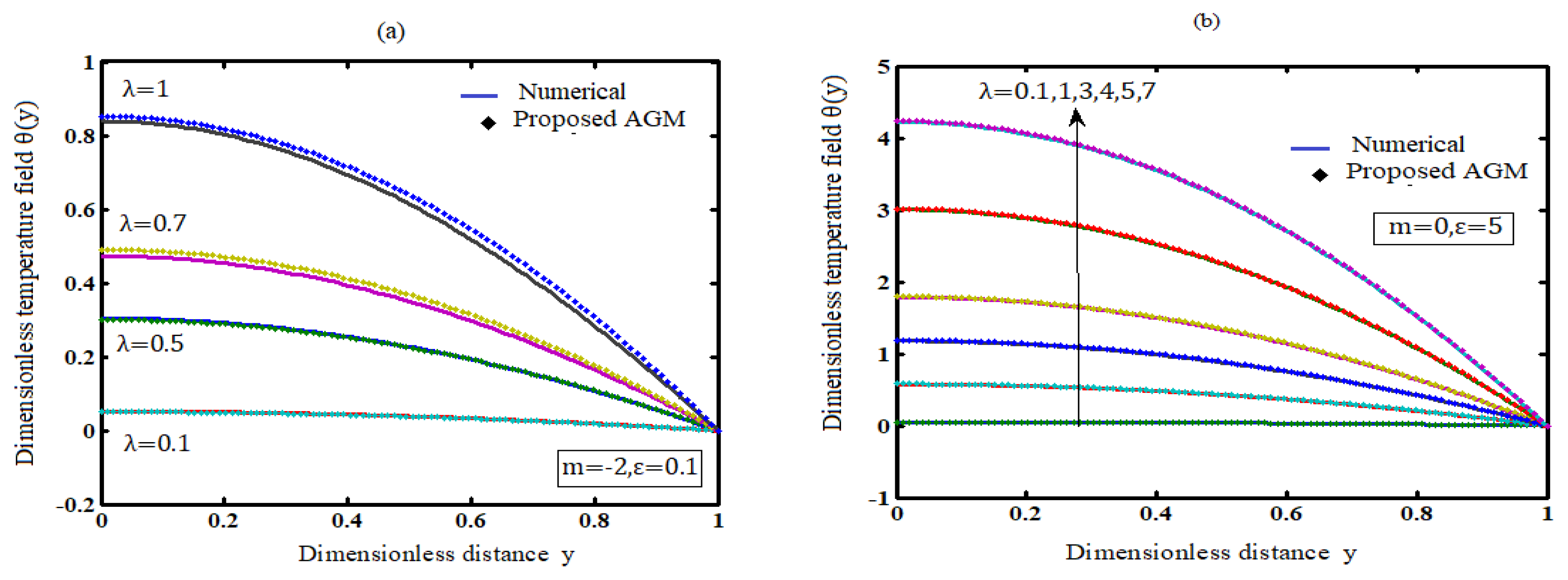
Figure 2.
Comparison of temperature field with simulation results (a) for various values of m (Kinetics) and (b) for various values of (Activation energy).
Figure 2.
Comparison of temperature field with simulation results (a) for various values of m (Kinetics) and (b) for various values of (Activation energy).
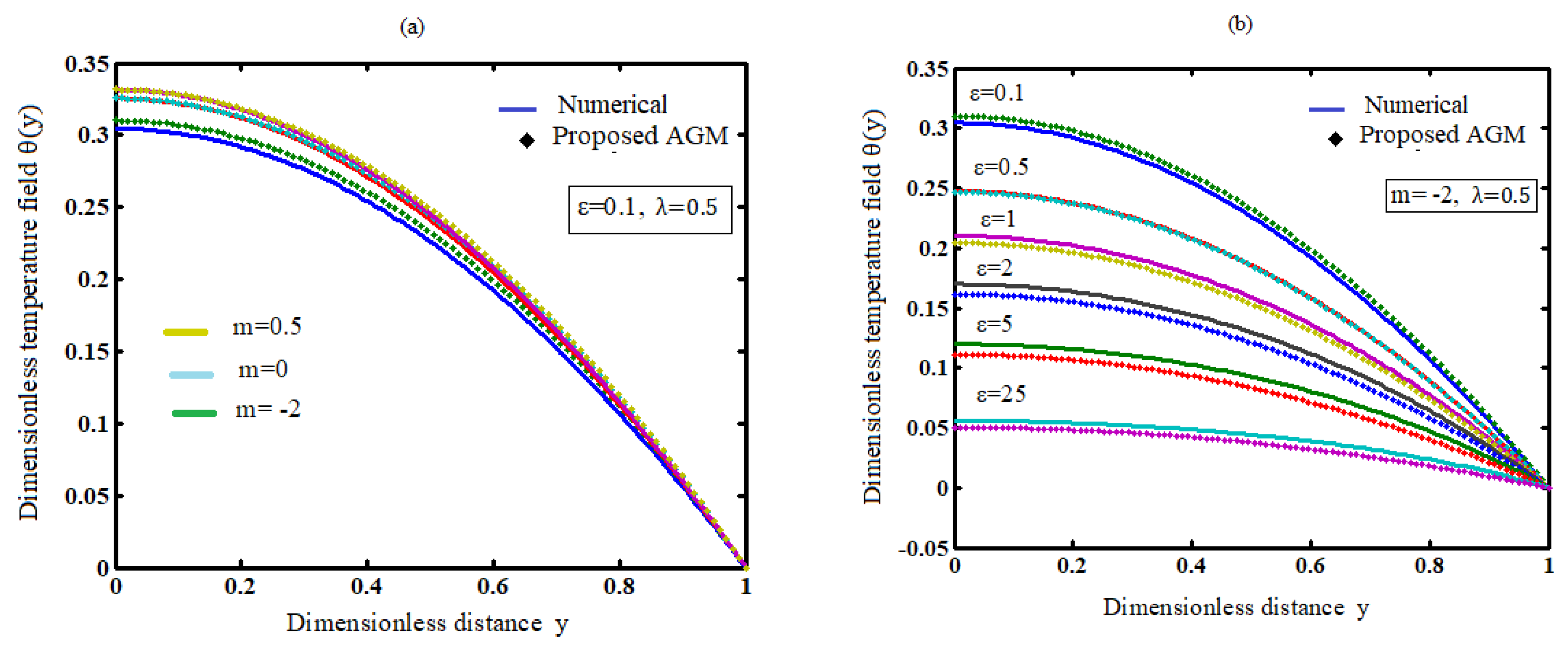
Table 1.
Comparison of the analytical results with numerical and earlier analytical results for the temperature when , .
Table 1.
Comparison of the analytical results with numerical and earlier analytical results for the temperature when , .
| Num. | AGM Eq. (12). This work |
HAM [11] Eq. (14) |
PM [10] Eq. (15) |
Error % AGM Eq. (12) This work |
Error % HAM [11] Eq. (14) |
Error % PM [10] Eq. (15) |
|
| 0 | 0.0517 | 0.0517 | 0.0517 | 0.0516 | 0.0000 | 0.0000 | 0.1934 |
| 0.2 | 0.0496 | 0.0496 | 0.0496 | 0.0495 | 0.0000 | 0.0000 | 0.2016 |
| 0.4 | 0.0432 | 0.0436 | 0.0434 | 0.0433 | 0.9259 | 0.0230 | 0.4629 |
| 0.6 | 0.0327 | 0.0324 | 0.0330 | 0.0329 | 0.9174 | 0.0303 | 0.6116 |
| 0.8 | 0.0179 | 0.0180 | 0.0185 | 0.0185 | 0.5586 | 3.3519 | 3.3519 |
| 1 | 0.0000 | 0.0000 | 0.0000 | 0.0000 | 0.0000 | 0.0000 | 0.0000 |
| Average error (%) | 0.3493 | 0.5675 | 0.8036 | ||||
Table 2.
Comparison of the analytical results with numerical and earlier analytical results for the temperature when , .
Table 2.
Comparison of the analytical results with numerical and earlier analytical results for the temperature when , .
| Num. | AGM Eq. (12). This work |
HAM [11] Eq. (14) |
PM [10] Eq. (15) |
Error % AGM Eq. (12) This work |
Error % HAM [11] Eq. (14) |
Error % PM [10] Eq. (15) |
||
| 0 | 0.3045 | 0.3201 | 0.2951 | 0.2823 | 4.8133 | 3.0870 | 7.2906 | |
| 0.2 | 0.2916 | 0.3001 | 0.2829 | 0.2707 | 2.8000 | 2.9835 | 7.1673 | |
| 0.4 | 0.2532 | 0.2548 | 0.2466 | 0.2363 | 0.6319 | 2.5671 | 6.6745 | |
| 0.6 | 0.1899 | 0.1893 | 0.1869 | 0.1792 | 0.3159 | 1.5798 | 5.6334 | |
| 0.8 | 0.1031 | 0.1030 | 0.1041 | 0.1002 | 0.0970 | 0.9699 | 2.8128 | |
| 1 | 0.0000 | 0.0000 | 0.0000 | 0.0000 | 0.0000 | 0.0000 | 0.0000 | |
| Average error (%) | 1.4430 | 1.8645 | 4.9298 | |||||
Table 3.
Comparison of the analytical results with numerical and earlier analytical results for the temperature when when .
Table 3.
Comparison of the analytical results with numerical and earlier analytical results for the temperature when when .
| Num. | AGM Eq. (12). This work |
HAM [11] Eq. (14) |
PM [10] Eq. (16) |
Error % AGM Eq. (12) This work |
Error % HAM [11] Eq. (14) |
Error % PM [10] Eq. (16) |
||
| 0 | 0.0522 | 0.0523 | 0.0521 | 0.0522 | 0.1916 | 0.1916 | 0.0000 | |
| 0.2 | 0.0501 | 0.0501 | 0.0500 | 0.0501 | 0.0000 | 0.1996 | 0.0000 | |
| 0.4 | 0.0436 | 0.0437 | 0.0437 | 0.0438 | 0.2294 | 0.2294 | 0.4587 | |
| 0.6 | 0.0329 | 0.0331 | 0.0332 | 0.0333 | 0.6079 | 0.9118 | 1.2158 | |
| 0.8 | 0.0180 | 0.0181 | 0.0188 | 0.0187 | 0.5555 | 4.4444 | 3.8889 | |
| 1 | 0.0000 | 0.0000 | 0.0000 | 0.0000 | 0.0000 | 0.0000 | 0.0000 | |
| Average error (%) | 0.2641 | 0.9961 | 0.9272 | |||||
Table 4.
Comparison of the analytical results with numerical and earlier analytical results for the temperature when , .
Table 4.
Comparison of the analytical results with numerical and earlier analytical results for the temperature when , .
| Num. | AGM Eq. (12). This work |
HAM [11] Eq. (14) |
PM [10] Eq. (16) |
Error % AGM Eq. (12) This work |
Error % HAM [11] Eq. (14) |
Error % PM [10] Eq. (16) |
|
| 0 | 0.3255 | 0.3208 | 0.3192 | 0.3172 | 1.4439 | 1.9355 | 2.5499 |
| 0.2 | 0.3116 | 0.3077 | 0.3059 | 0.3040 | 1.2516 | 1.8292 | 2.4390 |
| 0.4 | 0.2701 | 0.2684 | 0.2662 | 0.2646 | 0.6294 | 1.4439 | 2.0363 |
| 0.6 | 0.2021 | 0.2030 | 0.2011 | 0.1994 | 0.4433 | 0.4948 | 1.3360 |
| 0.8 | 0.1093 | 0.1113 | 0.1117 | 0.1110 | 1.8230 | 2.1958 | 1.5553 |
| 1 | 0.0000 | 0.0000 | 0.0000 | 0.0000 | 0.0000 | 0.0000 | 0.0000 |
| Average error (%) | 0.9319 | 1.3163 | 1.6527 | ||||
Disclaimer/Publisher’s Note: The statements, opinions and data contained in all publications are solely those of the individual author(s) and contributor(s) and not of MDPI and/or the editor(s). MDPI and/or the editor(s) disclaim responsibility for any injury to people or property resulting from any ideas, methods, instructions or products referred to in the content. |
© 2023 by the authors. Licensee MDPI, Basel, Switzerland. This article is an open access article distributed under the terms and conditions of the Creative Commons Attribution (CC BY) license (http://creativecommons.org/licenses/by/4.0/).
Copyright: This open access article is published under a Creative Commons CC BY 4.0 license, which permit the free download, distribution, and reuse, provided that the author and preprint are cited in any reuse.
Submitted:
05 July 2023
Posted:
21 July 2023
You are already at the latest version
Alerts
A peer-reviewed article of this preprint also exists.
This version is not peer-reviewed
Submitted:
05 July 2023
Posted:
21 July 2023
You are already at the latest version
Alerts
Abstract
This paper discusses the mathematical modelling of exothermic explosions in a slab. This model is based on a nonlinear equation containing a nonlinear term related to Arrhenius, bimolecular, and sensitised laws of reaction kinetics. The absolute temperature can be obtained by solving the nonlinear equation using Akbari-Ganji’s method. The influence of the parameters Frank-Kamenetskii, activation energy and numerical exponent on temperature is discussed. The analytical results are compared with previous available analytical and numerical results ( Matlab). A satisfactory agreement is noted.
Keywords:
Subject: Chemistry and Materials Science - Electrochemistry
1. Introduction
In explosive applications, the safety of combustible materials during transport and storage is essential. Self-ignition is a common occurrence with certain materials. This interior healing occurs when an explosive chemical is heated to a temperature where the decomposition process begins to cause significant exothermic effects. A thermal runaway effect occurs when the temperature rises rapidly, resulting in a fast thermal breakdown. Understanding the components that control this occurrence in many industrial processes is essential.
Many authors have provided models to explain thermal runaway and abusive behaviour. Hatchard et al. [1] make the first attempts to explain the exothermic reaction kinetics. In the works of Peng et al. [3,4] and Kim et al. [2] a simplified reaction-diffusion model is presented. There is also a discussion of an electrochemical model of lithium-ion battery nail absorption [5]. Wang et al. [6] present a catastrophe theoretic approach using a reduced ordinary differential equation model as a foundation. In [7], this model has been expanded. One must identify the primary exothermic chemical reactions to describe the thermal runaway of LIBs. Rising temperature can be used to describe the overall mechanism that causes a thermal runaway [1,3,4,8,9].
The equilibrium voltage and the method by which the equilibrium voltage is derived from the temperature are crucial factors in the electrochemical heat source [10]. The mechanisms of thermal abuse inside the Lithiyam- iron battery are directly related to modelling the thermal runaway and exothermic heat sources. As the temperature rises inside a battery, many exothermic chemical reactions may occur. If there is insufficient heat transmission to the environment [11] or if the rate of heat creation is higher than the heat dissipation rate, this could produce heat that accumulates inside the cell and speeds up the chemical reaction between the components of the cell. Any external factors, including outer heating, high or low voltage/current, nail piercing, exterior shorts, and others, might cause a temperature increase. Cells can be destroyed by a thermal runaway that can be brought on by an air leak, cigarette smoke, gas combustion, fires, etc. In 1930, Semonov, Zeldovith, and Frank Kamenetskii described this behaviour first, and their pioneering contributions are presented in [12]. Frank-Kamenetskii also proposed the steady-state theory of thermal explosion. This idea has been applied to various combustible material geometries in the literature. For the infinite slab, Boddington et al. [13,14,15] reviewed the case of two-step parallel exothermic processes, and they extended their research to include the geometries of the sphere and the circular cylinder.
Graham-Eagle et al. [16] studied a system of exothermic processes co-occurring. The critical values of the Frank-Kamenetskii parameter and the maximum temperature were calculated using a variational technique. The analysis of simultaneous processes [17] was expanded by the same authors to exothermic and endothermic reactions. Gelfand et al. [18] numerically determined the parameter's values.
Ajadi and Gol'dshtein [19] used a three-step kinetics of reactions model including steps for initiation, transmission, and cessation. The computation was performed using an approximation of the effective activation energy. The critical values for several geometries, including infinite square, rod, and cube, have been determined by Balakrishnan et al. [20] employing the finite difference method.
Makinde et al. [21] used the perturbation technique and Hermite-Pade approximants to arrive at the analytical solutions to the governing nonlinear boundary-value problem. They also explored the fundamental characteristics of the thermodynamic field, such as heat and bifurcations. Ananthasamy et al. [22] derived the analytical expression of temperature in exothermic explosions in a slab by solving the nonlinear equation using HAM. It is time-consuming since this contains an infinite number of convergence-control parameters.
Er-Riani and Chetehouna [23] apply the homotopy perturbation method for solving the steady-state nonlinear equation in an exothermic chemical reaction. This method was introduced by He [24,25,26]. In this communication, we derive the simple analytical expression for the temperature field for three kinds of reactions by solving the nonlinear equaftion using Akbari-Ganji’s method.
2. Problem Formulation and Analysis
Considering the steady-state of an exothermic chemical reaction in a combustible slab with the potential of heat loss to the environment. Frank-Kamenetskii [12] first proposed the classical formulation of this problem. The heat balance equation for steady-state conditions is given as follows:
The boundary conditions are
The material's thermal conductivity is denoted by the letters k, while T represents the absolute temperature. The other parameters have the same standard meaning as in the reference [12]. Additionally, the numerical exponent for Arrhenius, bimolecular, and sensitised kinetics is m = 2, 0, 1/2. To reduce the complexity, we make the nonlinear Eq. (1) into dimensionless form by defining the following dimensionless parameters.
where is the dimensionless temperature field, represents the Frank-Kamenetskii constant, denotes the activation energy. Using Eq. (4), the Eq. (1) reduces to the following dimensionless form.
The boundary conditions (2) and (3) can be reduced as folows:
3. Analytical Expression of the Temperature using Akbari-Ganji’s method
Recently, a variety of asymptotic techniques for solving nonlinear differential equations have been established such as the Adomian decomposition [27,28], Variational iteration [29,30], Taylor series [31,32] and Akbari-Ganji method (AGM) [33,34,35,36,37,38,39,40]. Among these techniques, AGM might be recognised as a useful algebraic (semi-analytic) method of resolving such problems. According to the AGM, a solution function with unidentified constant coefficients is supposed to satisfy the differential equation and the initial conditions. Then, the unknown coefficients are calculated using algebraic equations derived from initial conditions and derivatives.
We can assume that the trial solution of the Eq. (5) is
where are constants. We obtain the constant using the boundary conditions (6) and (7) as follows:
Now define the function by
Using Eq. (8), the Eq. (10) at becomes
Using eq. ( 9), the eq. (8) can be rewritten as follows:
The parameter is obtained by solving the nonlinear equation
The unidentified parameter in the equation (13) can be obtained with the Ying Buzu technique [41]. The value of this parameter was also determined using the regular false method and the secant algorithm. The Ying Buzu algorithm approach provides a convergent solution very quickly.
4. Previous analytical results
4.1. Homotopy analysis method
Anathaswamy et al. [11] used the homotopy analysis method (HAM) to solve Eq. (5) with boundary conditions (6) and (7). They obtained that the analytical expression for the temperature field
It takes a very long time since the convergence-control parameter h are unbounded.
4.2. Perturbation method
Makinde et al [10] solved Eq. (5) with boundary conditions (6) and (7) using the perturbation approach. According to their computations, the temperature was:
These approximate solutions are obtained by carrying out expansions in terms of a small parameter . In addition to this, perturbation method is not always to generate a continuous family of solutions in terms of the small parameter.
5. Discussion
Equation (12) represents the simplest analytical expression of the temperature profile. The thermal decomposition of the reacting combustible material depends on the parameters , which are of great importance for applications in explosives handling and industrial safety.
5.1. Numerical Simulation
This section validates the above theoretical results using numerical simulation for physically realistic values of various embedded parameters. The function bvp4c in Matlab/Scilab software, which solves non-linear boundary value problems for ordinary differential equations, is used to solve these equations numerically. The present (AGM) and previous (HAM, PM) analytical results are compared to this numerical solution in Table 1, Table 2, Table 3 and Table 4. The maximum average relative error between our result and the simulation result is 1.44. But the maximum error between numerical results and HAM and PM is 1.86% and 4.92%.
6. Limiting case
When the activation energy or Arrhenius kinetics (m) is very small, the equation (5) becomes
In this case, the temperature becomes,
where n is obtained from the equation
We can notice that the average error percentage between AGM and an exact limiting case result (eqn.(19)) does not exceed 1.8% for the slab.
Table 5.
Comparison of our approximate analytical result (12) with exact result (19) for the limiting case.
Table 5.
Comparison of our approximate analytical result (12) with exact result (19) for the limiting case.
| Exact solution |
AGM Eq. (12) |
Error% | Exact solution |
AGM Eq. (12) |
Error% | Exact solution |
AGM Eq. (12) |
Error% | |
| 0 | 0.0522 | 0.0527 | 0.9578 | 0.1733 | 0.1795 | 3.5776 | 0.3290 | 0.3474 | 5.5927 |
| 0.2 | 0.0501 | 0.0505 | 0.7984 | 0.1661 | 0.1689 | 1.6857 | 0.3148 | 0.3246 | 3.1131 |
| 0.4 | 0.0436 | 0.0439 | 0.6881 | 0.1443 | 0.1440 | 0.2079 | 0.2728 | 0.2768 | 1.4663 |
| 0.6 | 0.0329 | 0.0330 | 0.3039 | 0.1085 | 0.1087 | 0.1843 | 0.2040 | 0.2060 | 0.9804 |
| 0.8 | 0.0180 | 0.0180 | 0.0000 | 0.0590 | 0.0590 | 0.0000 | 0.1102 | 0.1102 | 0.0000 |
| 1 | 0.0000 | 0.0000 | 0.0000 | 0.0000 | 0.0000 | 0.0000 | 0.0000 | 0.0000 | 0.0000 |
| Average error (%) | 0.4580 | Average error (%) | 0.9426 | Average error (%) | 1.8587 | ||||
7. Influence of the parameters on temperature
7.1. Effect of the Frank-Kamenetskii parameter on temperature
Figure 1 illustrates the effects of the Frank-Kamenetskii parameter on a temperature profile. Figure 2 shows that an increase in Frank-Kamenetskii leads to an increase in the rate of an exothermic reaction. The maximum temperature along the slab is at the centre line, and the minimum is at the slab surface.. The slab temperature will invariably rise as a result of this.
7.2. Effect of the numerical exponent m on temperature
The effects of numerical exponent m on temperature profiles are shown in Figure 2 (a). The figure shows that the temperature increases as the numerical exponent number m increases. Moreover, the tables and figures show that in a bimolecular (m = 0.5) reaction, a thermal explosion occurs faster than in the Arrhenius (m = 0), sensitised (m = -2) reactions.
7.3. Effect of the activation energy parameter (ε) on temperature
A similar effect of temperature is observed with increasing values of activation energy parameter (ε) (Figure 2-b). With rising values of the activation energy, a similar effect of temperature enhancement is observed. Increasing values of ε imply that the reacting slab's activation energy is insufficient, and thus the reacting slab's volatility characteristic is significantly reduced.
8. Conclusions
We studied the exothermic explosion of a viscous combustible in the slab under various laws of reactions.The exothermic chemical reaction in a slab of flammable material is considered. The expected outcomes reveal that this method provides an outstanding and highly accurate approximation of the solution of this nonlinear system. The effects of the parameters Frank-Kamenetskii, numerical exponent of temperature and activation energy on temperature profiles are discussed. This method can be applied to infinite cylindrical and spherical geometries.
Funding
The authors have not received any funds.
Institutional Review Board Statement
Not applicable.
Informed Consent Statement
Not applicable.
Conflicts of Interest
The author declare no conflict of interest.
References
- Hatchard, T.D.; MacNeil, D.D.; Basu, A.; Dahn, J.R. Thermal model of cylindrical and prismatic lithium-ion cells. J. Electrochem. Soc 2001, 148, A755–A761. [Google Scholar] [CrossRef]
- Kim, G.H.; Pesaran, A.; Spotnitz, R. A three-dimensional thermal abuse model for lithium-ion cells. J. Power Sources 2007, 170, 476–489. [Google Scholar] [CrossRef]
- Peng, P.; Sun, Y.; Jiang, F. Thermal analyses of LiCoO2 lithium-ion battery during oven tests. Heat Mass Transf 2014, 50, 1405–1416. [Google Scholar] [CrossRef]
- Peng, P.; Sun, Y.; Jiang, F. Numerical simulations and thermal behavior analysis for oven thermal abusing of LiCoO2 lithium-ion battery. CIESC J 2014, 65, 647–657. [Google Scholar]
- Chiu, K.C.; Lin, C.H.; Yeh, S.F.; Lin, Y.H.; Chen, K.C. An electrochemical modeling of lithium-ion battery nail penetration. J. Power Sources 2014, 251, 254–263. [Google Scholar] [CrossRef]
- Wang, Q.; Ping, P.; Sun, J. Catastrophe analysis of cylindrical lithium ion battery. Nonlinear Dyn 2010, 61, 763–772. [Google Scholar] [CrossRef]
- Wang, Q.; Ping, P.; Zhao, X.; Chu, G.; Sun, J.; Chen, C. Thermal runaway caused fire and explosion of lithium ion battery. J. Power Sources 2012, 208, 210–224. [Google Scholar] [CrossRef]
- Lisbona, D.; Snee, T. A review of hazards associated with lithium and lithium-ion batteries. Process Saf. Environ. Prot 2011, 89, 434–442. [Google Scholar] [CrossRef]
- Abraham, D.P.; Roth, E.P.; Kostecki, R.; McCarthy, K.; MacLaren, S.; Doughty, D.H. Diagnostic examina tion of thermally abused high-power lithium-ion cells. J. Power Sources 2006, 161, 648–657. [Google Scholar] [CrossRef]
- Ziebert, C.; Melcher, A.; Lei, B.; Zhao, W.; Rohde, M.; Seifert, H.J. Chapter Six - Electrochemical–Thermal Characterization and Thermal Modeling for Batteries, Emerging Nanotechnologies in Rechargeable Energy Storage Systems. Micro and Nano Technologies 2017, 195–229. [Google Scholar]
- Guo, G.; Long, B.; Cheng, B.; Zhou, S.; Cao, B. Three-dimensional thermal finite element modeling of lithium-ion battery in thermal abuse application. J. Power Sources 2010, 195, 2393–2398. [Google Scholar] [CrossRef]
- Frank-Kamenetskii, D.A. Diffusion and Heat Transfer in Chemical Kinetics; Plenum Press: New York, NY, USA, 1969. [Google Scholar]
- Boddington, T.; Gray, P.; Robinson, C. Thermal explosions and the disappearance of criticality at small activation energies: Exact results for the slab. Proc. R. Soc. Lond 1979, 368, 441–461. [Google Scholar]
- Boddington, T.; Feng, C.G.; Gray, P. Thermal explosions, criticality and the disappearance of criticality in systems with distributed temperatures. I. arbitrary biot number and general reaction rate laws. Proc. R. Soc. Lond 1983, 390, 247–264. [Google Scholar]
- Boddington, T.; Gray, P.; Wake, G.C. Theory of thermal explosions with simultaneous parallel reactions. I. foundations and the one-dimensional case. Proc. R. Soc. Lond 1984, 393, 85–100. [Google Scholar]
- Graham-Eagle, J.G.; Wake, G.C. Theory of thermal explosions with simultaneous parallel reactions. II. The two- and three-dimensional cases and the variational method. Proc. R. Soc. Lond. A 1820, 401, 195–202. [Google Scholar]
- Graham-Eagle, J.G.; Wake, G.C. The theory of thermal explosions with simultaneous parallel reactions.III. Disappearance of critical behaviour with one exothermic and one endothermic reaction. Proc. R. Soc. Lond A 1986, 407, 183–198. [Google Scholar]
- Gelfand, I.M.; Fomin, S.V. Calculus of Variations; Prentice Hall: Englewood Cliffs, NJ, USA, 1963. [Google Scholar]
- Ajadi, S.O.; Gol’dshtein, V. Critical behaviour in a three-step reaction kinetics model. Combust. Theory Model 2009, 13, 1–16. [Google Scholar] [CrossRef]
- Balakrishnan, E.; Swift, A.; Ke, G.C. Critical values for some nonclass A geometries in thermal ignition theory. Mathl. Comput. Modelling 1996, 24, 1–10. [Google Scholar] [CrossRef]
- Makinde, O.D. Exothermic explosions in a slab: A case study of series summation technique. Int. Commun. Heat Mass Transf. 2004, 31, 1227–1231. [Google Scholar] [CrossRef]
- Ananthaswamy, V.; Subha, M. Analytical expressions for exothermic explosions in a slab. Int. J. Res. Granthaalayah 2014, 1, 22–33. [Google Scholar] [CrossRef]
- Er-Riani, M.; Chetehouna, K. On the critical behaviour of exothermic explosions in class A geometries. Math. Probl. Eng 2011, 536056, 1–14. [Google Scholar] [CrossRef]
- He, J.H. A coupling method of a homotopy technique and a perturbation technique for non-linear problems. Int J Non-Linear Mech 2000, 35, 37–43. [Google Scholar] [CrossRef]
- He, J.H. Homotopy perturbation method: A new nonlinear analytical technique. Appl. Math. Comput 2003, 135, 73–79. [Google Scholar] [CrossRef]
- He, J.H. Homotopy perturbation method for solving boundary value problems. Phys. Lett. A 2006, 350, 87–88. [Google Scholar] [CrossRef]
- Jeyabarathi, P.; Kannan, M.; Rajendran, L. Approximate analytical solutions of biofilm reactor problem in applied biotechnology. Theor. Found. Chem. Eng 2021, 55, 851–861. [Google Scholar] [CrossRef]
- Jeyabarathi, P.; Rajendran, L.; Abukhaled, M.; Kannan, M. Semi-analytical expressions for the concentrations and effectiveness factor for the three general catalyst shapes. React. Kinet. Mech. Catal. 2022, 1–16. [Google Scholar] [CrossRef]
- Abukhaled, M. Variational iteration method for nonlinear singular two-point boundary value problems arising in human physiology. J. Math 2013, 1–4. [Google Scholar] [CrossRef]
- He, J.H.; Wu, X.H. Variational iteration method: New development and applications. Comput. Math. with Appl 2007, 54, 881–894. [Google Scholar] [CrossRef]
- Vinolyn Sylvia, S.; Joy Salomi, R.; Rajendran, L.; Abukhaled, M. Solving nonlinear reaction–diffusion problem in electrostatic interaction with reaction-generated pH change on the kinetics of immobilized enzyme systems using Taylor series method. J. Math. Chem 2019, 59, 1332–1347. [Google Scholar] [CrossRef]
- He, J.H. Taylor series solution for a third order boundary value problem arising in Architectural Engineering. Ain Shams Eng. J. 2022, 11, 1411–141. [Google Scholar] [CrossRef]
- Jeyabarathi, P.; Rajendran, L.; Lyons, M.E.G.; Abukhaled, M. Theoretical Analysis of Mass Transfer Behavior in Fixed-Bed Electrochemical Reactors: Akbari-Ganji’s Method. Electrochem 2022, 3, 699–712. [Google Scholar] [CrossRef]
- Joy Salomi, R.; Vinolyn Sylvia, S.; Rajendran, L.; Abukhaled, M. Electric potential and surface oxygen ion density for planar, spherical and cylindrical metal oxide grains. Sens. Actuators B Chem 2020, 321, 128576. [Google Scholar] [CrossRef]
- Manimegalai, B.; Lyons, M.E.G.; Rajendran, L. A kinetic model for amperometric immobilized enzymes at planar, cylindrical and spherical electrodes: The Akbari-Ganji method. J Electroanal Chem 2021, 880, 114921. [Google Scholar] [CrossRef]
- Mary, M.; Chitra Devi, M.; Meena, A.; Rajendran, L.; Abukhaled, M. Mathematical modeling of immobilized enzyme in porous planar, cylindrical, and spherical particle: A reliable semi-analytical approach. React. Kinet. Mech. Catal 2021, 1–11. [Google Scholar] [CrossRef]
- Jeyabarathi, P.; Rajendran, L.; Lyons, M.E.G. Reaction-diffusion in a packed-bed reactors: Enzymatic isomerization with Michaelis-Menten kinetics. J Electroanal Chem 2022, 910, 11618. [Google Scholar] [CrossRef]
- Akbari, M.R.; Ganji, D.D.; Goltabar, A.R. Solving nonlinear differential equations of Vanderpol, Rayleigh and Duffing by AGM. Front. Mech. Eng 2014, 9, 177–190. [Google Scholar] [CrossRef]
- Rostami, A.K.; Akbari, M.R.; Ganji, D.D.; Heydari, S. Investigating Jeff ery-Hamel flow with high magnetic field and nanoparticle by HPM and AGM. Cent. Eur. J. Eng 2014, 4, 357–370. [Google Scholar]
- Meresht, N.B.; Ganji, D.D. Solving nonlinear differential equation arising in dynamical systems by AGM. Int. J. Appl. Comput. Math 2017, 3, 1507–1523. [Google Scholar] [CrossRef]
- Manimegalai, B.; Swaminathan, R.; Lyons, M.E.G.; Rajendran, L. Application of Taylor’s series with Ying Buzu Shu algorithm for the nonlinear problem in amperometric biosensors. Int. J. Electrochem. Sci. 2022, 17, 22074. [Google Scholar] [CrossRef]
Figure 1.
Comparison of analytical expression of temperature field with simulation results for different values of Frank-Kamenetskii parameter using eq. (12).
Figure 1.
Comparison of analytical expression of temperature field with simulation results for different values of Frank-Kamenetskii parameter using eq. (12).
Figure 2.
Comparison of temperature field with simulation results (a) for various values of m (Kinetics) and (b) for various values of (Activation energy).
Figure 2.
Comparison of temperature field with simulation results (a) for various values of m (Kinetics) and (b) for various values of (Activation energy).
Table 1.
Comparison of the analytical results with numerical and earlier analytical results for the temperature when , .
Table 1.
Comparison of the analytical results with numerical and earlier analytical results for the temperature when , .
| Num. | AGM Eq. (12). This work |
HAM [11] Eq. (14) |
PM [10] Eq. (15) |
Error % AGM Eq. (12) This work |
Error % HAM [11] Eq. (14) |
Error % PM [10] Eq. (15) |
|
| 0 | 0.0517 | 0.0517 | 0.0517 | 0.0516 | 0.0000 | 0.0000 | 0.1934 |
| 0.2 | 0.0496 | 0.0496 | 0.0496 | 0.0495 | 0.0000 | 0.0000 | 0.2016 |
| 0.4 | 0.0432 | 0.0436 | 0.0434 | 0.0433 | 0.9259 | 0.0230 | 0.4629 |
| 0.6 | 0.0327 | 0.0324 | 0.0330 | 0.0329 | 0.9174 | 0.0303 | 0.6116 |
| 0.8 | 0.0179 | 0.0180 | 0.0185 | 0.0185 | 0.5586 | 3.3519 | 3.3519 |
| 1 | 0.0000 | 0.0000 | 0.0000 | 0.0000 | 0.0000 | 0.0000 | 0.0000 |
| Average error (%) | 0.3493 | 0.5675 | 0.8036 | ||||
Table 2.
Comparison of the analytical results with numerical and earlier analytical results for the temperature when , .
Table 2.
Comparison of the analytical results with numerical and earlier analytical results for the temperature when , .
| Num. | AGM Eq. (12). This work |
HAM [11] Eq. (14) |
PM [10] Eq. (15) |
Error % AGM Eq. (12) This work |
Error % HAM [11] Eq. (14) |
Error % PM [10] Eq. (15) |
||
| 0 | 0.3045 | 0.3201 | 0.2951 | 0.2823 | 4.8133 | 3.0870 | 7.2906 | |
| 0.2 | 0.2916 | 0.3001 | 0.2829 | 0.2707 | 2.8000 | 2.9835 | 7.1673 | |
| 0.4 | 0.2532 | 0.2548 | 0.2466 | 0.2363 | 0.6319 | 2.5671 | 6.6745 | |
| 0.6 | 0.1899 | 0.1893 | 0.1869 | 0.1792 | 0.3159 | 1.5798 | 5.6334 | |
| 0.8 | 0.1031 | 0.1030 | 0.1041 | 0.1002 | 0.0970 | 0.9699 | 2.8128 | |
| 1 | 0.0000 | 0.0000 | 0.0000 | 0.0000 | 0.0000 | 0.0000 | 0.0000 | |
| Average error (%) | 1.4430 | 1.8645 | 4.9298 | |||||
Table 3.
Comparison of the analytical results with numerical and earlier analytical results for the temperature when when .
Table 3.
Comparison of the analytical results with numerical and earlier analytical results for the temperature when when .
| Num. | AGM Eq. (12). This work |
HAM [11] Eq. (14) |
PM [10] Eq. (16) |
Error % AGM Eq. (12) This work |
Error % HAM [11] Eq. (14) |
Error % PM [10] Eq. (16) |
||
| 0 | 0.0522 | 0.0523 | 0.0521 | 0.0522 | 0.1916 | 0.1916 | 0.0000 | |
| 0.2 | 0.0501 | 0.0501 | 0.0500 | 0.0501 | 0.0000 | 0.1996 | 0.0000 | |
| 0.4 | 0.0436 | 0.0437 | 0.0437 | 0.0438 | 0.2294 | 0.2294 | 0.4587 | |
| 0.6 | 0.0329 | 0.0331 | 0.0332 | 0.0333 | 0.6079 | 0.9118 | 1.2158 | |
| 0.8 | 0.0180 | 0.0181 | 0.0188 | 0.0187 | 0.5555 | 4.4444 | 3.8889 | |
| 1 | 0.0000 | 0.0000 | 0.0000 | 0.0000 | 0.0000 | 0.0000 | 0.0000 | |
| Average error (%) | 0.2641 | 0.9961 | 0.9272 | |||||
Table 4.
Comparison of the analytical results with numerical and earlier analytical results for the temperature when , .
Table 4.
Comparison of the analytical results with numerical and earlier analytical results for the temperature when , .
| Num. | AGM Eq. (12). This work |
HAM [11] Eq. (14) |
PM [10] Eq. (16) |
Error % AGM Eq. (12) This work |
Error % HAM [11] Eq. (14) |
Error % PM [10] Eq. (16) |
|
| 0 | 0.3255 | 0.3208 | 0.3192 | 0.3172 | 1.4439 | 1.9355 | 2.5499 |
| 0.2 | 0.3116 | 0.3077 | 0.3059 | 0.3040 | 1.2516 | 1.8292 | 2.4390 |
| 0.4 | 0.2701 | 0.2684 | 0.2662 | 0.2646 | 0.6294 | 1.4439 | 2.0363 |
| 0.6 | 0.2021 | 0.2030 | 0.2011 | 0.1994 | 0.4433 | 0.4948 | 1.3360 |
| 0.8 | 0.1093 | 0.1113 | 0.1117 | 0.1110 | 1.8230 | 2.1958 | 1.5553 |
| 1 | 0.0000 | 0.0000 | 0.0000 | 0.0000 | 0.0000 | 0.0000 | 0.0000 |
| Average error (%) | 0.9319 | 1.3163 | 1.6527 | ||||
Disclaimer/Publisher’s Note: The statements, opinions and data contained in all publications are solely those of the individual author(s) and contributor(s) and not of MDPI and/or the editor(s). MDPI and/or the editor(s) disclaim responsibility for any injury to people or property resulting from any ideas, methods, instructions or products referred to in the content. |
© 2023 by the authors. Licensee MDPI, Basel, Switzerland. This article is an open access article distributed under the terms and conditions of the Creative Commons Attribution (CC BY) license (http://creativecommons.org/licenses/by/4.0/).
Copyright: This open access article is published under a Creative Commons CC BY 4.0 license, which permit the free download, distribution, and reuse, provided that the author and preprint are cited in any reuse.
Modeling of a Double Gas Hydrate Particle Ignition
Olga Gaidukova
et al.
Applied Sciences,
2022
Theoretical Prediction Model of the Explosion Limits for Multi-Component Gases (Multiple Combustible Gases Mixed with Inert Gases) under Different Temperatures
Qiuju Ma
et al.
Fire,
2022
Three-Dimensional Numerical Modeling of Internal Ballistics for Solid Propellant Combinations
Ramón Otón-Martínez
et al.
Mathematics,
2021


MDPI Initiatives
Important Links
© 2024 MDPI (Basel, Switzerland) unless otherwise stated