Evaluation of Wear Models for the Wear Calculation of Journal Bearings for Planetary Gears in Wind Turbines

Preprint

Article

Evaluation of Wear Models for the Wear Calculation of Journal Bearings for Planetary Gears in Wind Turbines

Altmetrics

Downloads

208

Views

Comments

A peer-reviewed article of this preprint also exists.

Benjamin Lehmann^*

,Philipp Trompetter,

Francisco Gutiérrez Guzmán,

Georg Jacobs

Benjamin Lehmann^*

,Philipp Trompetter,

Francisco Gutiérrez Guzmán,

Georg Jacobs

This version is not peer-reviewed

Submitted:

20 July 2023

Posted:

24 July 2023

You are already at the latest version

Alerts

Abstract

To increase the power density of the electromechanical drive train of wind turbines, journal bearings can be used as planetary gear bearings instead of rolling bearings. This technological change presents new challenges. For example, wind turbine drive systems are subject to dynamic and low-speed operating conditions which can lead to an accelerated abrasive wear of the journal bearings. In addition, oil supply failure or peak loads due to wind gusts and grid and power converter faults could potentially result in catastrophic failure due to adhesive wear in a very short time. Such operating characteristics are, therefore, critical regarding the journal bearing wear lifetime and must be considered in the design. The successful implementation of journal bearings in wind turbines depends on a reliable estimation of adhesive and abrasive wear. In this paper, five different models for the wear calculation of journal bearings are evaluated regarding their suitability of wear calculation of planetary gear bearings in wind turbines. For this purpose, the following evaluation criteria were defined: parameter uncertainty, parametrization effort, in particular number of parameters, parameterization method and load case dependency of parameters and calculation effort. In order to be able to evaluate the wear models, the wear models are numerically implemented and the wear of a test journal bearing is exemplarily calculated under load conditions, which are comparable to load conditions in a wind turbine. Relevant influences from the wind turbine system such as lubricant, material and manufacturing dependent surface influences like roughness and hardness are considered. The wear models are evaluated with respect to their fulfillment of the defined criteria. The resulting evaluation allows the selection of a wear model that can be used to calculate the wear of planetary gear journal bearings in wind turbines, considering the available input variables.

Keywords:

Subject: Engineering - Mechanical Engineering

1. Introduction

Wear is the progressive loss of material from the surface of a body caused by tribological stress [1]. Depending on the structure of the tribological system and the kinematics of the tribological stress, a distinction is made between different types of wear. Due to dynamic and slow-speed operating conditions journal bearings in wind turbines are generally subject to sliding wear. According to Czichos [1], the four wear mechanisms for journal bearings are adhesion, abrasion, micro fatigue and tribochemical reaction. In order to be able to predict the bearing wear analytically, different approaches have been developed in the past, which are based on different wear mechanisms. Holm [2] developed a wear approach, by assuming the contact between atoms of opposing surfaces as the cause of wear. Archard [3] developed this approach further and considered not the contact of atoms, but the contact and the resulting plastic deformation of asperity peaks of the surfaces. Rowe [4] extended the model developed by Archard to include the influence of the lubricant used in the wear calculation. Chun [5] used the model created by Rowe to simulatively predict wear of journal bearings in starting and stopping operations of a reciprocating engine. Besides Archard, the most widely used model for wear calculation is the energetic approach developed by Fleischer [6]. In this approach, it is assumed that friction energy is generated during the sliding process, which is accumulated in the material. If the accumulated energy has reached a critical limit, the lattice energy of the material is overcome and wear occurs.

The wear models according to Archard and Rowe assume a linear wear process in their calculation. However, when observing real wear processes in journal bearings, a deviation from this prediction can be observed. It can be seen that the rate of wear is initially higher than the one predicted by the linear wear calculations and only approaches the wear behavior of the linear forecasts after a run-in phase has been completed [7]. Simultaneously with the change in the rate of wear, the coefficient of friction also changes. In lubricated friction contacts, the friction process usually starts with increased coefficients of friction until wear leads to a smoothing of the surfaces and the value of the coefficient of friction decreases [8].

In the recent past, attempts have been made to take the running-in phase of a journal bearing into account in the wear calculation and thus to be able to predict the entire course of wear more accurately. In Fleischer's wear approach, the behavior of the friction coefficient is not specified in more detail. Therefore, Fleischer's wear approach can be implemented both linearly, with a time-constant friction coefficient, and with transient behavior, using a time-varying friction coefficient. König [8], using Fleischer's approach, developed a numerical method for wear prediction of journal bearings under start-stop conditions, iteratively considering both the journal bearing wear at macroscopic level and at roughness level. In this way, a simulative prediction of run-in wear became possible using the Fleischer approach. By means of the developed method, agreements of the journal bearing wear in the running-in process between simulation and experiment could be shown. Nevertheless, the approach according to König requires an iterative adjustment of the friction coefficient of Fleischer's wear approach, which changed continuously during the running-in process. Additionally, the input parameters of the model were based on roughness measurements, some of which were subject to large scatter. Another approach that enables transient wear calculation was developed by Xiang et al. In this approach, two mechanisms are assumed to contribute to wear [9]. First, wear is considered to be caused by the plastic deformation of asperity peaks in contact; this affects the material above contact surface. On the other hand, it is assumed that fatigue cracks develop below the contact surface and lead to the breakout of material after a certain accumulation. As an alternative to these mechanical approaches, the wear approach according to Lijesh [10] based on the work of Bryant [11] takes a thermodynamic approach to describe wear. The free enthalpy is assumed to decrease in proportion to the degradation of the tribological system until an equilibrium state is reached at the minimum free enthalpy. Since the decrease in free enthalpy is coupled to the generation of entropy, the increase of entropy is regarded as the driving variable of wear in the model. The wear behavior is described with the aid of a degradation coefficient, which sets the wear volume created in relation to the entropy produced. Independently of the previous approaches, Cao et al. [12] developed a method for calculating adhesive wear, which is based on the assumption that a wear particle is formed during the wear process, which detaches from the surface and thus leads to material loss at the surface. The size of the wear particle and the time of detachment are subject to a statistical distribution. To map the statistical distribution, Cao et al. introduced a numerical criterion that calculates the probability that a wear particle will form and be detached. A major uncertainty in the approach according to Cao et al. is the determination of the mean surface energy of the contact partners and its standard deviation, as well as the determination of the material-specific maximum work of adhesion. A summary of the wear approaches for journal bearing wear calculation is shown in Table 1.

As shown in Table 1, the presented wear approaches consider different damage mechanism responsible for the wear. In addition, only some models allow the consideration of a transient wear rate. Furthermore, the approaches use partly physically based parameters and partly empirical parameters to describe the wear of the system. As a result, different wear approaches are expected to be suitable for different applications or varying tribological systems. So far, it is not known which of the wear approaches is best suited for describing the wear in planetary gears of wind turbines. Therefore, in this paper the different wear approaches are screened, implemented and evaluated regarding their suitability for the wear calculation of planetary gear bearings in wind turbines. In this study, only the slow progressing wear process is addressed. However, the frictional heat generated by severe adhesion events can also lead to critical operating conditions and even to spontaneous failure of the plain bearings. This damage mechanism will be considered in subsequent studies.

2. Approach

In order to identify the best suited approach for describing the wear in planetary gears of wind turbines, the different wear approaches presented in section 1 are tested at the Institute for Machine Elements and Systems Engineering with the aim to select a suitable approach for the wear calculation and subsequently to be able to reliably predict the wear of planetary gear bearings in wind turbines. The procedure is divided into five steps and shown in Figure 1. First, the wear approaches are screened, implemented and evaluated (step 1). Then, calculations of the wear progress are performed from a radially loaded journal bearing using the different wear approaches (step 2). The results are then compared with experimental results generated on a component test rig (step 3). The component test rig allows several bearings to be tested in a short time and under defined conditions. In this way, sufficient test data is collected to parameterize and validate the wear approaches. On the component test rig, wear conditions are also considered, which lead to fretting of the bearing. Materials and lubricants used in real wind turbines are used for the experimental tests on the component test rig. Steps 1 to 3 result in a wear approach and a methodology with which the wear behavior of the test bearing can be reliably predicted, initially under radial load. Subsequently, the methodology is applied to a model of a gearbox test rig (step 4). The gearbox test rig reproduces real load conditions in wind turbines. In order to consider the real load conditions in the simulative wear prediction, it is extended for the locally resolved wear calculation of planetary gear bearings. The results of the simulative wear prediction are then compared with test data from the gearbox test rig (step 5). In this way, it can be evaluated whether the selected wear approach and the developed method are suitable for the wear calculation of planetary gear bearings under real load conditions or whether further development needs are necessary. In combination with the simultaneously published work "Simulation methodology for the identification of critical operating conditions of planetary journal bearings in wind turbines", both studies represent the first steps towards the development of a framework for the use of planetary journal bearings in wind turbines.

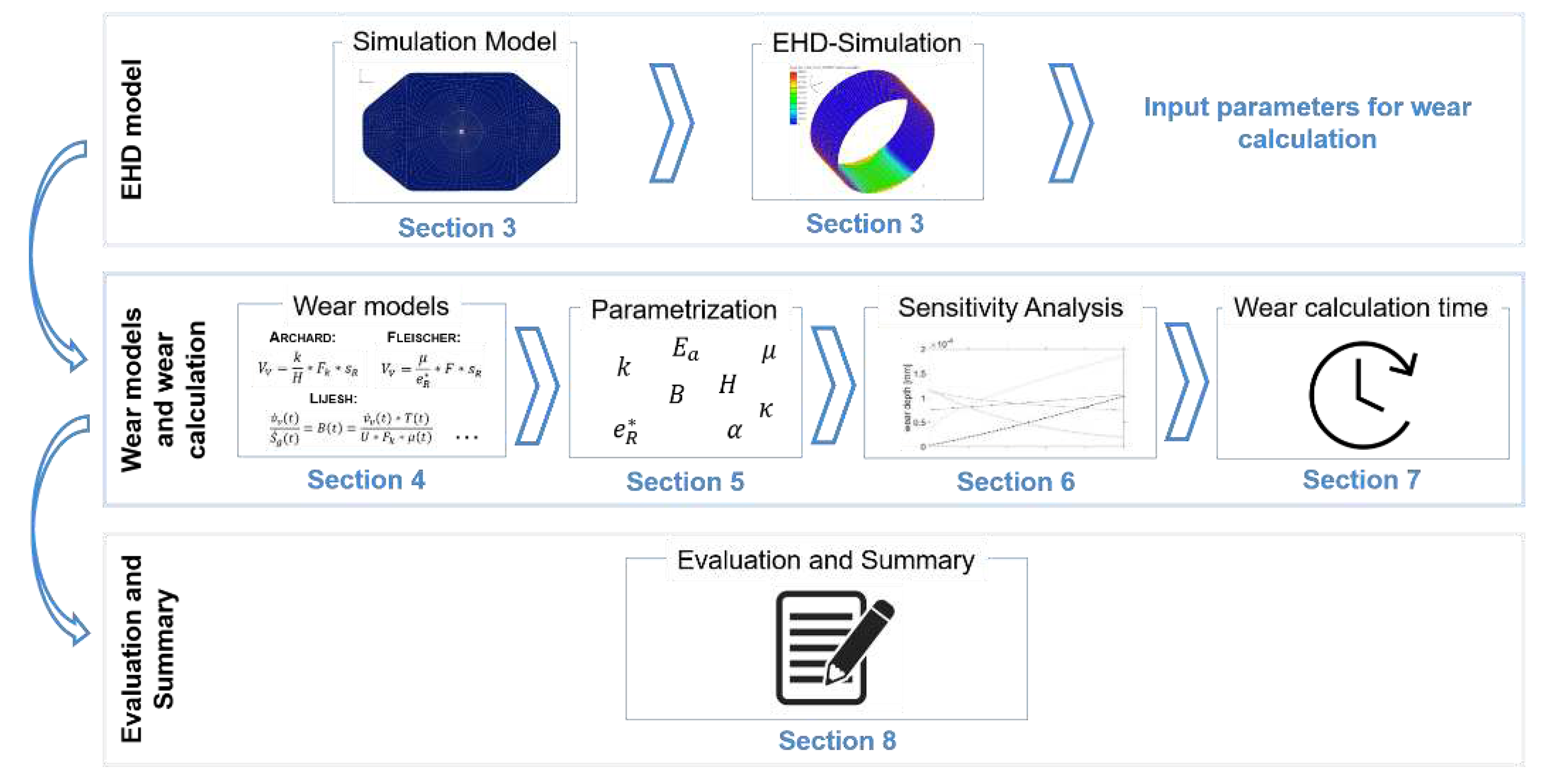
This study addresses the screening, implementation and evaluation of the wear approaches (Step 1) and wear calculations of the component test rig bearing (Step 2) considering materials and lubricants used in wind turbines. The approach of the study is shown in Figure 2. First, EHD simulations of the component test rig are performed to simulatively determine the contact conditions in the journal bearing, which provide the input parameters for the wear calculations. Subsequently, the wear models and the procedures for their parameterization are presented in detail. This is followed by sensitivity analyses to evaluate the parameter uncertainties and analyses of the calculation time of the different wear approaches. Finally, the wear approaches are evaluated with respect to their suitability for wear calculation.

3. Journal Bearing Test Rig and EHD Simulation Model

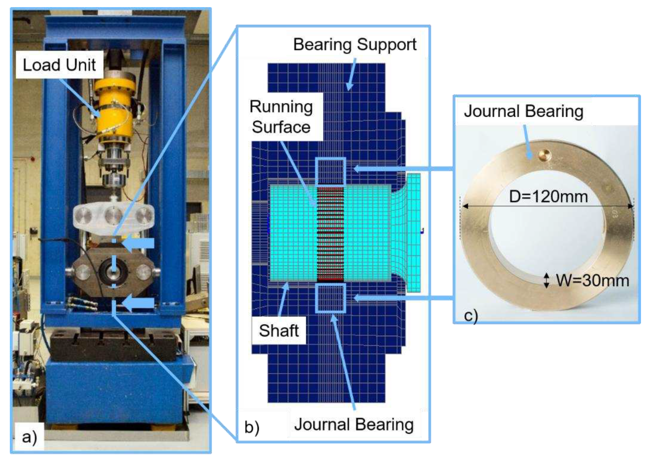
In addition to material and lubricant properties, the resulting contact conditions within the journal bearing, such as solid contact pressure and lubricant film height at a defined load condition, are input variables for the wear calculation. In order to determine the contact conditions of a test bearing, an EHD/MBS model was built. The EHD/MBS model reproduces an existing component test rig at the Institute for Machine Elements and Systems Engineering of the RWTH Aachen University (Figure 3a). The shaft is supported by two supporting bearings. The test bearing (Figure 3c) is mounted torsionally rigid in the bearing support. The bearing support is designed as a friction balance in order to be able to record frictional torques acting in the journal bearing. The test bearing is pulled against the shaft by the load unit. A 250 kN servo-hydraulic cylinder is used as the load unit. During the tests, the following quantities can be recorded:

-: Radial force
-: Shaft speed
-: Bearing temperature
-: Friction torque

The built EHD/MBS simulation model comprises the test bearing, the shaft and the surrounding structure for bearing support (Figure 3b). The geometrical and material-specific data of the test bearing and the shaft as well as data of the oil used are given in Table 2. The materials and oil correspond to those used in wind turbines, whereas additivation of the oil cannot be considered in the simulation model.

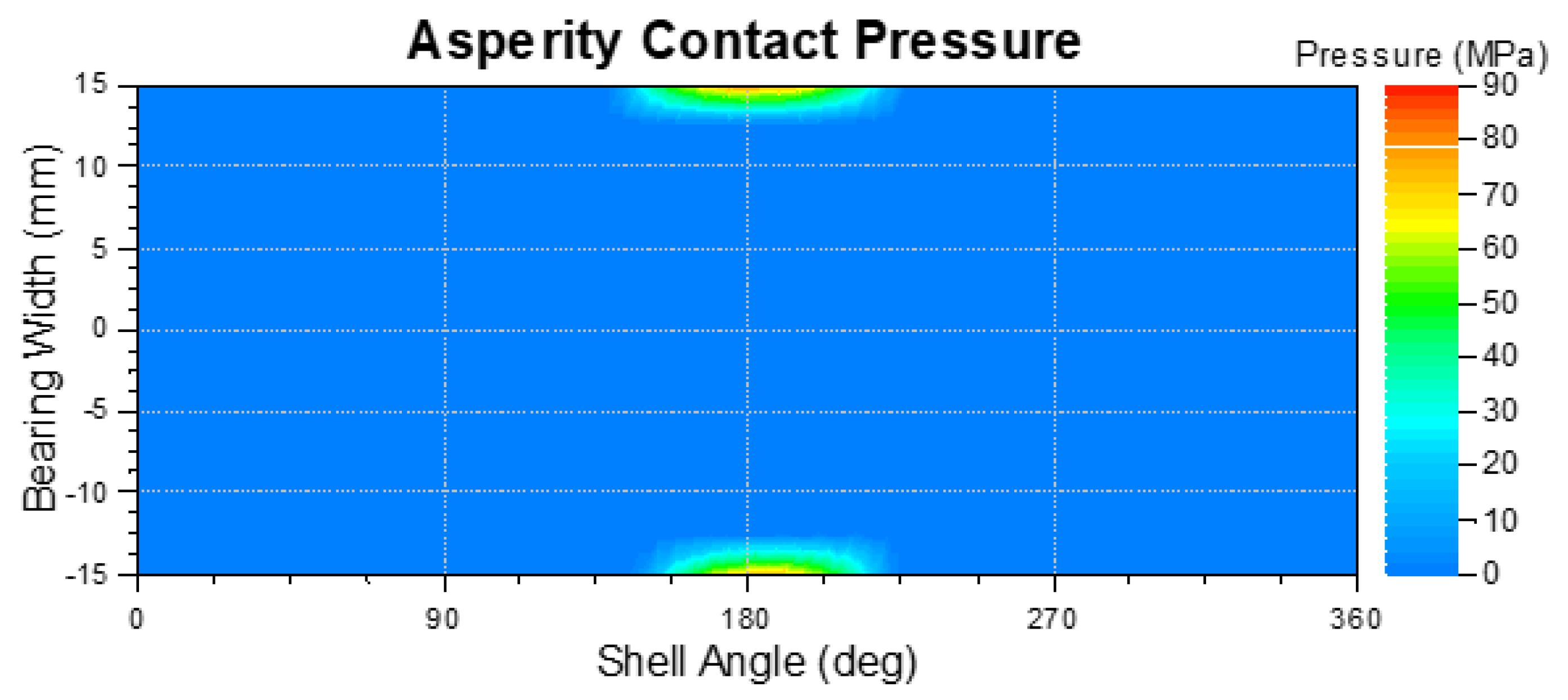
In order to be able to calculate wear occurring in planetary gear journal bearings, wear-critical conditions must be generated at circumferential speeds, which occur in wind turbines today. Therefore, in the EHD/MBS simulation a constant normal force of 200 KN at a speed of 100 rpm (specific pressure of 55 MPa and a circumferential speed of 0.628 m/s) was applied as the load. The result of the EHD/MBS simulation are the solid contact pressure occurring in the bearing, the asperity contact ratio and the height of the lubricant film, which are used as input variables for the wear calculation. The distribution and height of the solid contact pressure over the bearing surface for the given load condition are shown in Figure 4. The solid contact pressure initially occurs at the bearing edges. Due to the radially acting load, the two areas of maximum solid contact pressure are at 180° shell angle. Although edge bearing loading also occurs in planetary gear bearings, the maximum loaded zones are not directly opposite each other. Therefore, the load condition shown in Figure 4 is only an approximation of real load conditions occurring in planetary journal bearings.

4. Implementation of the Wear Models

The wear approaches according to Arachard, Fleischer, Chun, Lijesh and Xiang were implemented and coupled with the EHD/MBS simulation of the test bearing (see section 3). Since the approaches according to Holm, Rowe and Bryant only represent preliminary development stages of the previously mentioned approaches, they are not considered further. In addition, the model according to Cao et al. is not considered, since it requires a complex initial 3D surface microanalysis and has so far only been applied for point contacts. In the following, the underlying equations and the parameters of the wear approaches mentioned and implemented at the beginning will be discussed.

In the approach according to Archard [13] the wear volume is related to the contact force acting on a body

F_{k}

, the sliding distance

s_{R}

, the reciprocal of the hardness

H

and a proportionality factor

k

. The proportionality factor

k

describes the probability of material removal due to plastic deformation of the asperity peaks. Assuming the wear mechanism remains unchanged,

k

assumes time constant values for constant load cases. The wear volume is calculated as:

V_{V} = \frac{k}{H} * F_{k} * s_{R}

Chun's wear approach is based on the approach of Rowe [4], who introduces the parameter

Ψ

, which describes the ratio of real contact area to nominal contact area. The difference between these areas is caused by lubricant molecules adsorbed on the surface, which prevent direct metallic contact. Rowe developed this approach examining wear behavior using n-hexadecane as a lubricant, allowing to include the influence of the lubricant in the wear calculation.

Ψ

is calculated by:

Ψ = 1 - \exp (\frac{X}{U * t_{0}} * e^{- \frac{E_{a}}{R * T}})

The values used for calculation are derived from the chemical properties of the lubricant and describe how many of the molecules adsorbed on the rough metal surface are displaced by oncoming asperity peaks.

X

is the diameter which is affected by a molecule adsorbed on the surface,

t_{0}

is the period of vibration of a lubricant molecule adsorbed on the surface,

R

the molar gas constant and

E_{a}

the adsorption energy.

U

is the relative sliding velocity between the two surfaces and

T

the temperature of the lubricating film. Integrating

Ψ

into the formula previously defined by Archard for calculating wear, results in:

V_{V} = Ψ * \frac{k}{H} * F_{k} * s_{R}

Fleischer [6] assumes in his approach that frictional energy is generated during the sliding process, which is accumulated in the material until a critical limit is reached. This is described by the friction energy density

e_{R}^{*}

which represents the ratio of wear volume created and the frictional energy responsible. Following this approach, the wear volume can be represented considering the friction coefficient

μ

as follows:

V_{V} = \frac{μ}{e_{R}^{*}} * F_{k} * s_{R}

As previously described, Xiang's approach considers two wear mechanisms [9]. The fraction of wear due to plastic deformation of asperity peaks in contact (this concerns the material which experiences deformation) is calculated with:

Δ V_{1, i} = \frac{π * δ_{a, i}^{2} * (3 β - δ_{a, i})}{3}

β

represents the asperity radius and

δ_{a, i}

is the plastic deformation of the asperity peaks in contact, which is determined by the Hertzian contact theory considering the average force affecting a single asperity

F_{a v, i}

δ_{a, i} = {(\frac{9 * F_{a v, i}^{2}}{16 * β * {E^{*}}^{2}})}^{\frac{1}{3}}

In order to calculate the proportion of fatigue cracks developing below the contact surface, which propagate along the angle

α

and lead to material breaking out after a certain accumulation, the following formula is used:

Δ V_{2, i} = \frac{2}{3} * π * \tan (α) * β^{\frac{2}{3}} * δ_{a, i}^{\frac{3}{2}}

In order to be able to map the transient wear progression during the running-in phase, the wear is calculated for a previously defined sliding cycle, the relevant parameters of the wear calculation are updated and the calculation is performed again. This is done until the end of a pre-defined wear period is reached. The wear within cycle i is calculated by:

V_{i} = \frac{N_{i}}{n_{i}} * (Δ V_{1, i} + Δ V_{2, i})

n_{i}

is the number of contact cycles between asperity peaks necessary for material removal due to fatigue.

n_{i} = {(\frac{σ_{b} * A_{r, i}}{3 * μ * F_{k, i}})}^{κ}

The solid contact force

F_{k, i}

and the real contact area

A_{r, i}

are calculated with the help of the statistical model of Greenwood and Williamson [14] for the description of rough surfaces. Here, a statistical normal distribution of asperities is assumed in order to be able to describe the solid contact as a function of the lubricant film thickness. As the lubricant film height changes due to wear and as a result of roughness smoothing, the solid contact force and the real contact area change in each sliding cycle. The parameters tensile strength

σ_{b}

, coefficient of friction

μ

and fatigue exponent

κ

are nevertheless assumed by Xiang to be constant throughout the wear process. The fatigue coefficient

κ

was established by Tan [15] and is an empirical exponent to describe the fatigue behavior. At this time the availability of values for

κ

is very limited. Only some experiments for nonmetallic materials and 1045 steel were conducted.

N_{i}

is used to describe the number of asperity contacts that occur within the i-th sliding cycle. For the calculation of

N_{i}

the contact model according to Greenwood and Tripp [16] is used:

N_{i} = 2 * A_{n, i} * D^{2} * β * Δ L * \int_{h_{c, i}}^{\infty} ϕ (k^{'}) d k'

N_{i}

depends on the current lubricant film height

h_{c, i}

and changes with each sliding cycle.

A_{n, i}

is the nominal contact area,

D

is the asperity density on the surface,

Δ L

is the sliding distance in one cycle, and

ϕ (k^{'})

is a Gaussian normal distribution.

The degradation coefficient presented by Lijesh [17] puts the wear rate

{\dot{v}}_{v}

in relation to the rate of entropy production

{\dot{S}}_{g}

and is calculated according to the following formula:

\frac{{\dot{v}}_{v} (t)}{{\dot{S}}_{g} (t)} = B (t) = \frac{{\dot{v}}_{v} (t) * T (t)}{U * F_{k} * μ (t)}

By using a time-dependent degradation coefficient, it is possible to map the transient behavior of the tribosystem during the run-in phase. The change in temperature is caused by the frictional heat generated, so the time dependent temperature profile is dependent on the friction coefficient.

When the wear calculation approaches developed by Fleischer and Lijesh were used, the Coefficient of Friction was calculated using the following formula by Offner and Knaus [18] describing the friction in mixed lubrication regimes:

μ_{l o k a l} = μ_{C o u l o m b} \cdot e^{- \sqrt{b \cdot L_{N}}} + c \cdot r_{c} \cdot L_{N} \cdot (1 - e^{- \sqrt{b \cdot L_{N}}})

The required values were taken from the work of KÖNIG [7].

5. Parameterization of the Wear Models

All of the wear approaches presented here follow a physical approach, but contain empirical parameters that require prior determination. The methods and consequently the effort of parameter determination differ between the wear approaches. In the following the necessary steps to determine the parameters of each wear approach are examined to allow for an assessment of the overall effort for complete parameterization. All parameters of the considered wear approaches and their respective methods for determination are therefore presented in Table 3.

Common to all the approaches mentioned is that an experimental trial is required to determine at least one parameter. Pin on disc experiments are a commonly used method. In pin on disc experiments, both the wear and the coefficient of friction can be measured. Based on the experiment results, the wear coefficient

k

for Archard and Chun and the wear-specific friction work according to Fleischer can be determined. However, it was shown that these parameters are dependent on the applied load, which is why a measurement for each load case, which is to be considered, is necessary for an accurate prediction of the wear [10, 20].

Lijesh developed the approach of a time-varying degradation coefficient in order to be able to map the transient running-in wear. To determine this coefficient, it is necessary to experimentally determine the wear rate and the coefficient of friction with regard to their time dependency. One way to continuously measure wear is to incorporate a differential transformer into pin on disc experiments [23]. It has been shown that the wear of different load cases can be determined sufficiently accurately by a constant degradation coefficient as long as the acting friction force is known for the load cases [10]. Thus, the one-time determination of the degradation coefficient B applying a constant load is sufficient.

Since Xiang's work uses the Greenwood and Williamson contact model as the basis of the wear calculation, this wear approach requires the parameters asperity density

D

and asperity radius

β

to describe the rough surface. Although these parameters change in the course of the wear process, constant values are assumed in the calculation, which is why a measurement of the surface on a journal bearing in new condition is sufficient. In this case, a 2D profile is sufficient to form the average values required for the calculation. The propagation angle of the fatigue fracture cannot be determined before the wear occurs, so a value between 15° and 30° must be estimated [9]. To determine the fatigue coefficient, an experimental determination of the wear, e.g. by a pin on disc test, is necessary. As with the degradation coefficient B, it has been shown that the variations in the wear results at different load cases are sufficiently small that a single determination of the fatigue coefficient at constant load is sufficient. [15]

The wear approach according to Chun requires, in addition to the wear coefficient known from Archard, information about the lubricant used. The vibration time of a lubricant film molecule in the adsorbed state can be calculated under the assumption that this vibration time is equal to the lattice vibration time of the adsorbing metal surface [24]. The vibration time can be calculated using the Lindemann formula [25]:

t_{0} = 4.75 * 10^{- 13} * \sqrt{\frac{M * V_{m}^{\frac{2}{3}}}{T_{m}}}

For this purpose, the molar mass M, the molar volume

V_{m}

and the absolute melting point

T_{m}

of the metal surface are required. For most materials, these values can be assumed to be known. Assuming that the molecular chains of the lubricant are arranged horizontally in all directions relative to the direction of movement of the asperity peaks, a circular area can be assumed to be affected by one molecule. [4] The diameter

χ

can be derived from the cross-sectional area affected by an lubricant molecule considering its length, 1.27n+2 Å for alkanes with n being the number of carbon atoms [22], and the distance between adjacent lubricant chains. The value of the adsorption energy can be derived from the friction value of pin-on-disc experiments at a constant temperature. [21] Due to the dependence of the coefficient of friction on the acting load, the adsorption heat is also load-dependent.

In summary, all approaches require a Pin-on-Disc Experiment, altough it could be argued that the the parameters of the long standing approaches Archard, Fleischer and Rowe are well known and should be seen as parameters found in literature. However, since the parameters are highly dependent on the circumstances considered, e.g. applied load, lubrication regime, material pairing, etc., prior experimental determination is recommended for accurate prediction of wear. Considering the effort of the necessary experiments alone, the parameter determination of the wear approach according to Lijesh shows the greatest complexity. The determination of the degradation coefficient B requires a temporal resolution of the wear, while for the remaining wear approaches the wear state at the end of the experiment is sufficient. In return the degradation coefficient B is independent of the applied load case, which is why a single experiment is sufficient to determine B for several load cases. The wear approach according to Xiang requires the biggest ammount of parameters, which contributes to the overall parameterization effort. Analogue to Lijesh these parameters are however independent of the load case. In order to determine the total effort necessary for complete parameterization of the wear approaches, the wear approaches can be rated in the categories „number of parameters“, „load dependency of parameters“ and „complexity of parameter determination“ using the overview provided in this chapter.

6. Sensitivity Analysis of the Wear Parameters

In the following, the sensitivity of the approaches to possible measurement deviations during the experiments for parameter determination or other parameter uncertainties will be evaluated. For this purpose, a local quantitative sensitivity analysis is performed according to the one-at-a-time principle. Here, one parameter is varied between limits obtained by literature research, while constant reference values are assumed for the remaining parameters. The selected number of variance points per parameter is

i = 50

. Due to lack of experimental data needed to determine all relevant parameters, the reference parameters were chosen within the researched limits such that the same maximum wear depth resulted from the different approaches. The reference wear depth was determined based on the Fleischer wear approach, utilizing the friction energy density determined by König [7]. The chosen limits, as well as the reference values, can be found in Table 4. The solid contact pressure and the height of the lubricant film required for the wear calculation are taken from the EHD simulation in section 3.

The magnitude and units of the wear parameters differ significantly. Therefore a comparison by simple local derivation is not possible, since a large sensitivity would follow from parameters of small magnitude and a very low sensitivity from parameters of large magnitude. Instead, the sensitivity of the wear calculation is compared using a dimensionless value that represents the relative change of the parameters. The following methodology, described by e.g. Hamby [29], was used: The difference in wear depth between two adjacent variance points was formed and divided by the reference wear depth. In addition, the difference between the associated parameter values was formed and was also divided by the associated reference parameter. This allows a comparison of the sensitivities despite different magnitudes. The sensitivity values were thus calculated as follows:

\bar{H_{w e a r}} = \frac{H_{w e a r} (i) - H_{w e a r} (i - 1)}{H_{w e a r, r e f}}

\bar{P} = \frac{P (i) - P (i - 1)}{P_{r e f}}

F = \frac{\bar{H_{w e a r}}}{\bar{P}}

For further comparison, the maximum value of

F

was determined for each parameter and used to compare the sensitivity of the calculated wear depth due to parameter deviations. The maximum values of

F

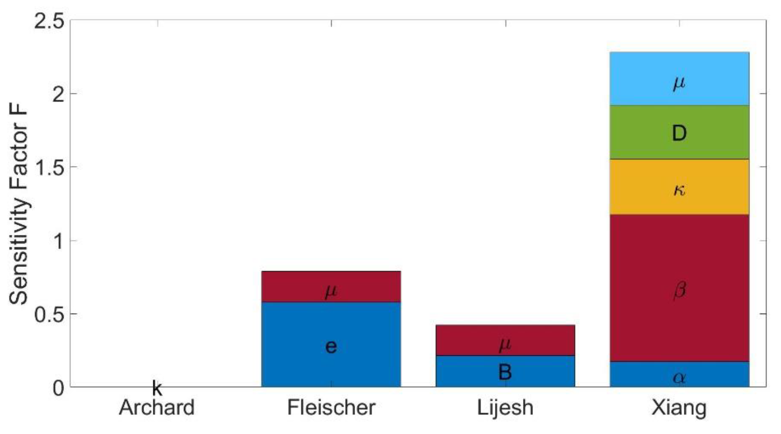
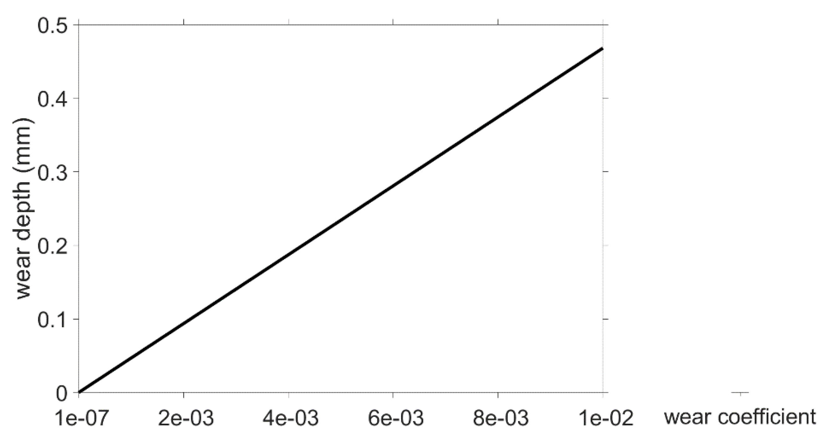
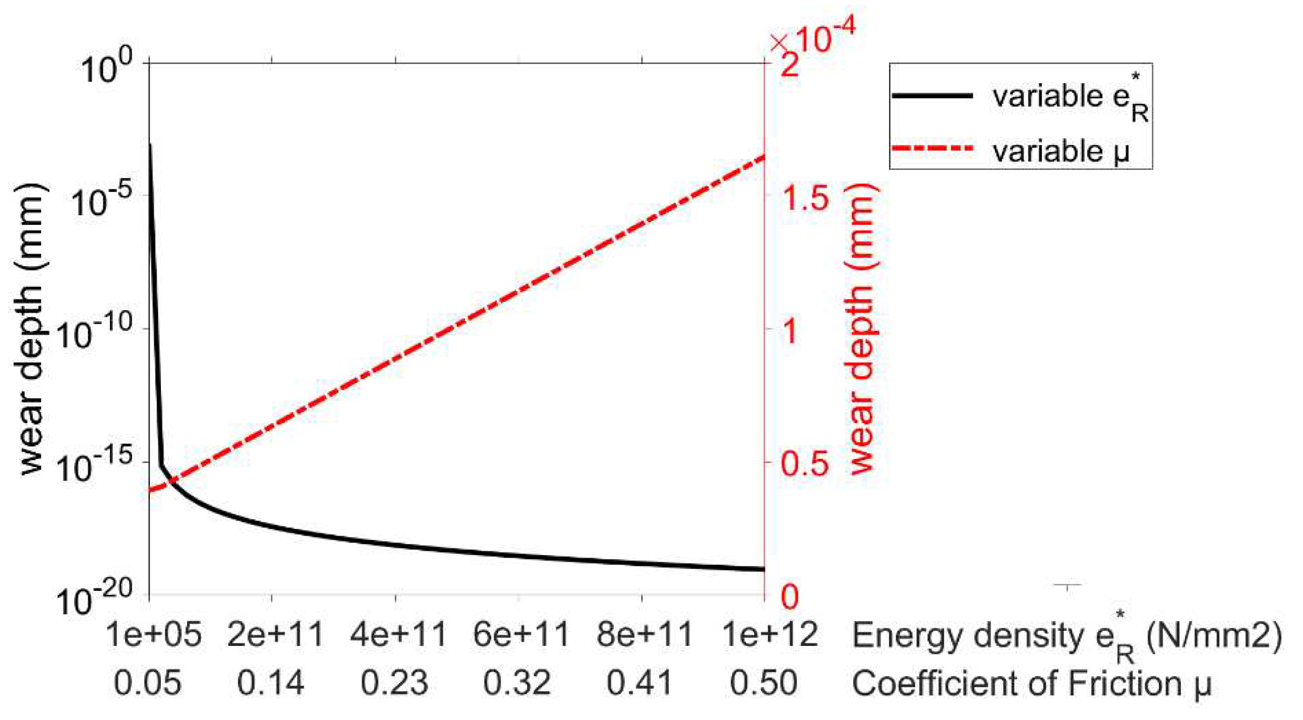
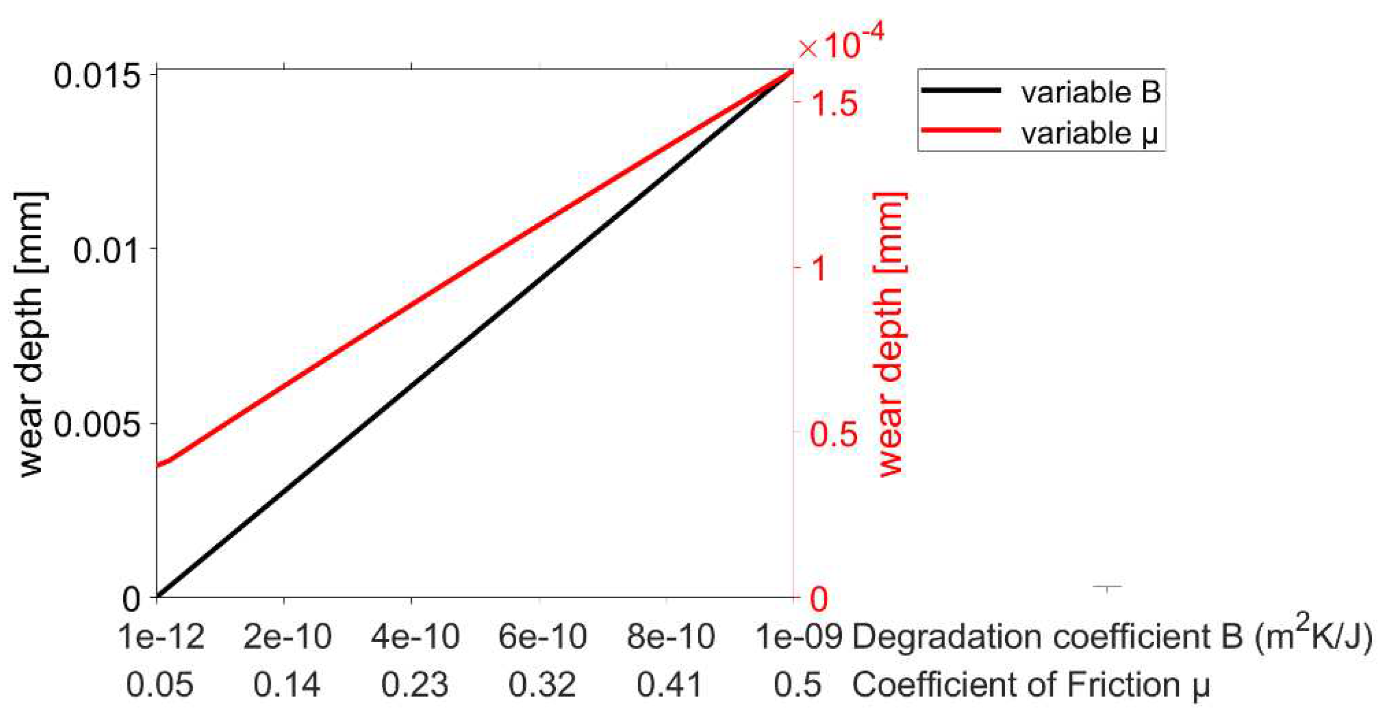
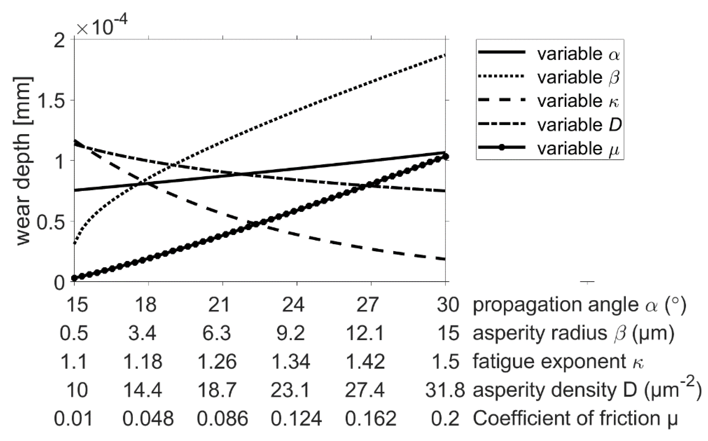
were then scaled to values between 0 and 1 using the min-max- normalization [30]. Then the values of the parameters of each model were added to determine a total sensitivity. Going forward the resulting sum will be called sensitivity factor. The sensitivity factors of the wear approaches are shown in Figure 5. The sensitivities of the individual wear approaches as a function of their input parameters are shown in Figure 6, Figure 7, Figure 8 and Figure 9.

To increase the readability of the graphs depicting the sensitivity of the Lijesh and Fleischer wear approach a second axis wih a deviating scaling has been introduced to allow the clear representation of all parameter influences, although the resulting wear depth differs in its order of magnitude.

Since k is only included as a constant prefactor in the Archard wear calculation, a linear increase in the wear height proportional to k follows. Lijesh also shows a relatively low sensitivity to a change in the parameters B and μ as the relationship between the wear height and the calculation parameters also follows a linear course. The wear approach of Fleischer shows a slightly greater sensitivity. The wear is proportional to the reciprocal of the friction energy density, so a regressive decrease in the maximum wear height is seen with increasing

e_{R}^{*}

. The overall sensitivity of the wear approach according to Xiang is considerably greater than that of the approaches mentioned so far (see Figure 5). This is partly due to the high number of parameters required. However especially the asperity radius β shows a slightly greater sensitivity than the other parameters.

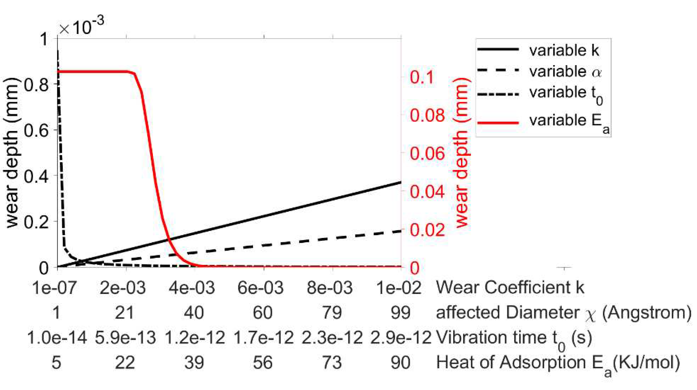
The wear approach according to Chun was not included in the previous analysis. This is due to the fact that this approach has a sensitivity whose difference to the remaining wear approaches is so large that a comparison with the previously mentioned methodology using the sensitivity factor will lead to negligible sensitivities of the other wear approaches due to the used min-max normalization. Figure 10 shows the curves of the wear depth as a function of the parameters for the approach according to Chun. The parameters wear coefficient k and diameter influenced by the adsorbed lubricant film molecule

χ

follow a linear course and exhibit relatively low sensitivity. The vibration time

t_{0}

is included in the denominator of the relevant equation, resulting in a high sensitivity at values close to the researched lower limit. However, the largest contribution to the sensitivity of Chun's model is made by the adsorption energy of the lubricant. As can be seen, there is a range for this parameter in which even very small changes cause a very large fluctuation in the wear level. When considering the curve of the wear depth, it should be noted that the graph for the adsorption energy

E_{a}

refers to the right axis of the diagram. The right axis was scaled up by a factor of aproximately 100 to be able to map the sensitivity in the graph. The reason for the massive sensitivity of

E_{a}

is the double exponential influence on the calculated wear.

7. Calculation Time

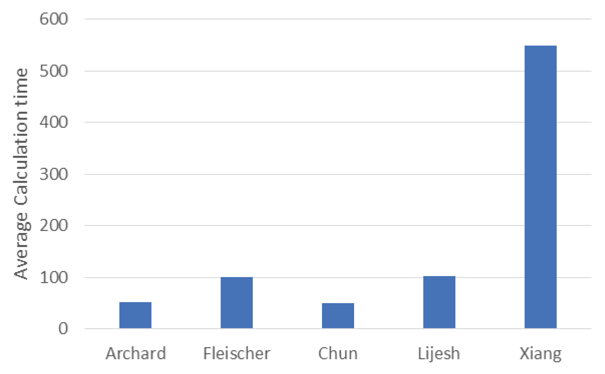
With regard to a fast provision of results, it is necessary to evaluate the duration of the wear calculation. This gains importance especially when severall iterative calculations are conducted. To compare the calculation time, 3 calculations were performed for each wear approach and the time required was measured. The basis for these calculations were the results of the EHD simulation (see section 3). The FE mesh used consists of 38 points in the circumferential direction of the bearing and 13 points across the width of the bearing. This results in 719*38*13=355186 data points considering a total rotation angle of 719° and a time increment of 1° rotation angle. The calculation was performed by an Intel Core i5-7600 3.5 GHz quad core CPU using Matlab R2018b. The exact results are shown in Table 5. Additionally, for a visually comparison the mean values of the results are shown in Figure 11.

The lowest time needed for calculation can be obtained using the approach according to Archard and Chun. The reason for this is the simplicity of the equations used and the need of only the solid contact pressure as an input for the calculation. Most of the calculation time is due to processing of result files. In the calculations according to Lijesh and Fleischer the lubrication gap height is required in addition to the solid contact pressure in order to calculate the coefficient of friction using the formular of Offner and Knaus. Accordingly, the number of required files is doubled and the data processing consequently takes about twice as long. The computation time of the approach according to Xiang is considerably larger in comparison to the other approaches. This is due to the integrals contained in the formulas used, which require considerably more computing time than the simple algebraic equations of the remaining models.

8. Summary and Outlook

The aim of this study was a screening, implementation and evaluation of different wear approaches regarding their suitability for the wear calculation of planetary gear bearings in wind turbines. Five different wear approaches (according to Archard, Fleischer, Chun, Lijesh and Xiang) were evaluated with respect to their suitability for the wear calculation of planetary gear bearings in wind turbines. For this purpose, an MBS/EHD simulation model was set up, which calculates the wear-relevant variables such as solid contact pressure, fluid contact pressure, shear rate and lubricant film height. Bearing materials and lubricating oils, which are commonly used in wind turbines, were considered. Subsequently, the five wear approaches were implemented. All of the wear approaches follow a physical approach, but contain empirical parameters that require prior determination. Therefore, all parameters of the considered wear approaches, their respective methods for determination and additionally their limit values were presented in tables. Subsequently sensitivity analyses were performed. The inputs of the sensitivity analysis were results of the MBS/EHD calculation. The results of the sensitivity analysis allow a conclusion on the parameter uncertainty, which is a criterion for the evaluation of the wear approaches. In addition, the methods for parameter determination, the number of parameters, the load case dependency and the calculation time are further criteria for the evaluation of the wear approaches.

The results show that regarding parameter uncertainty, Archard, Fleischer, and Lijesh present good approaches. Xiang’s approach, on the other hand, has a higher parameter uncertainty and can therefore lead to strong deviations in the wear calculation. In the approach according to Chun, the adsorption energy parameter has an extreme sensitivity and therefore leads to the highest parameter uncertainty. The approach according to Lijesh is the overall best approach for wear calculation according to the previously mentioned evaluation criteria. This is due to the fact that this approach achieves good results in almost all areas considered. Its calculation time is adequately low and the sensitivity of the parameters is lower than that of most other approaches. Its biggest disadvantage is the relatively elaborate experiment necessary for the parameterization, requiring a continuous measurement of the wear volume, which can e.g. be achieved by integrating a linear variable differential transducer. This disadvantage is however compensated by the load case indepency of the determined parameters, giving the approach a huge adventage when examining multiple occurring conditions leading to wear.

In the near future, the further steps mentioned in Figure 1 will be tackled. Currently, calculations of the local contour change and roughness change of the componenent test rig journal bearing are performed using the presented wear approaches. This has the aim of evaluating the wear approaches with respect to their agreement with experimental data (step 3). The agreement with experimental data will then represent a further criterion for the evaluation of wear models. Furthermore, real load situations will be considered for the wear calculation in the future (step 4), a method for wear calculation under real load conditions will be developed and the method will then be validated using experimental data from a gearbox test rig (step 5).

Author Contributions

Conceptualization, methodology, writing—review and editing, Benjamin Lehmann; conceptualization, methodology, writing—original draft preparation, Philipp Trompetter; writing—review and editing, Francisco Gutiérrez Guzmán; supervision, Georg Jacobs.

Funding

This research was funded by Federal Ministry for Economic Affairs and Climate Action of Germany. Preprints 80090 i001

Acknowledgments

We thank our project partners, who provided equipment, insight and expertise that greatly assisted the research.

Conflicts of Interest

The authors declare no conflict of interest.

References

Czichos H (2010) Tribologie-Handbuch: Tribometrie, Tribomaterialien, Tribotechnik, 3., überarbeitete und erweiterte Auflage. Springer eBook Collection Computer Science & Engineering. Vieweg+Teubner, Wiesbaden.
Holm R (1946) Electric contacts. Alquvist & Wiksells Akademisk Handböker. Gebers, Stockholm.
Archard JF (1953) Contact and Rubbing of Flat Surfaces. Journal of Applied Physics 24:981–988. [CrossRef]
Rowe CN (1966) Some Aspects of the Heat of Adsorption in the Function of a Boundary Lubricant. A S L E Transactions 9:101–111. [CrossRef]
Chun SM, Khonsari MM (2016) Wear simulation for the journal bearings operating under aligned shaft and steady load during start-up and coast-down conditions. Tribology International 97:440–466. [CrossRef]
Fleischer G (1980) Verschleiß und Zuverlässigkeit, 1st edn. Verlag Technik.
König F (2020) Prognose des Verschleißverhaltens ölgeschmierter Gleitlager: Wear Prediction of Plain Bearings under Mixed Friction Conditions. Dissertation, RWTH Aachen.
König F, Ouald Chaib A, Jacobs G et al. (2019) A multiscale-approach for wear prediction in journal bearing systems – from wearing-in towards steady-state wear. Wear 426-427:1203–1211. [CrossRef]
Xiang G, Han Y, Wang J et al. (2019) Coupling transient mixed lubrication and wear for journal bearing modeling. Tribology International 138:1–15. [CrossRef]
Lijesh KP, Khonsari MM (2018) On the Modeling of Adhesive Wear with Consideration of Loading Sequence. Tribol Lett 66. [CrossRef]
Bryant M, Khonsari M, Ling F (2008) On the thermodynamics of degradation. Proc R Soc A 464:2001–2014. [CrossRef]
Cao H, Tian Y, Meng Y (2021) A Fracture-Induced Adhesive Wear Criterion and its Application to the Simulation of Wear Process of the Point Contacts under Mixed Lubrication Condition. FU Mech Eng 19:23. [CrossRef]
Archard JF (1956) The wear of metals under unlubricated conditions. Proc R Soc Lond A 236:397–410. [CrossRef]
J.A. Greenwood, J.B.P. J.A. Greenwood, J.B.P. Williamson (1966) Contact of nominally flat surfaces. Proc R Soc Lond A 295:300–319. [CrossRef]
Tan Y, Zhang L, Hu Y (2015) A Wear Model of Plane Sliding Pairs Based on Fatigue Contact Analysis of Asperities. Tribology Transactions 58:148–157. [CrossRef]
Greenwood JA, Tripp JH (1970) The Contact of Two Nominally Flat Rough Surfaces. Proceedings of the Institution of Mechanical Engineers 185:625–633. [CrossRef]
Lijesh KP, Khonsari MM, Kailas SV (2018) On the integrated degradation coefficient for adhesive wear: A thermodynamic approach. Wear 408-409:138–150. [CrossRef]
Offner G, Knaus O (2015) A Generic Friction Model for Radial Slider Bearing Simulation Considering Elastic and Plastic Deformation. Lubricants 3:522–538. [CrossRef]
Yuqin W, Jinyuan T, Wei Z (2020) Influence of distribution parameters of rough surface asperities on the contact fatigue life of gears. Proceedings of the Institution of Mechanical Engineers, Part J: Journal of Engineering Tribology 234:821–832. [CrossRef]
Meier V, Illner T (2013) Gleitlagerverschleißgrenzen - Einsatzgrenzen von hydrodynamischen Weißmetallgleitlagern infolge von Verschleiß: Abschlussbericht. Lehrstuhl und Institut für Maschinenelemente und Maschinengestaltung.
Kingsbury EP (1958) Some Aspects of the Thermal Desorption of a Boundary Lubricant. Journal of Applied Physics 29:888–891. [CrossRef]
Kurtz SS, Jr. , Brooks BT, Boord CE et al. (1954) The chemistry of petroleum hydrocarbons 1. Reinhold, New York.
J. AR, Pottirayil A, Kailas SV (2017) Dry Sliding Wear Behavior of Ti-6Al-4V Pin Against SS316L Disk at Constant Contact Pressure. Journal of Tribology 139. [CrossRef]
Boer JH de (1968) The dynamical character of adsorption, 2nd ed. Clarendon P, Oxford.
Lindemann FA (1910) The calculation of molecular vibration frequencies. Physikalische Zeitschrift.:609– 612.
AVL List GmbH (2020) AVL Excite User Manual.
Leighton M, Morris N, Gore M et al. (2016) Boundary interactions of rough non-Gaussian surfaces. Proceedings of the Institution of Mechanical Engineers, Part J: Journal of Engineering Tribology 230:1359–1370. [CrossRef]
Kingsbury EP (1960) The Heat of Adsorption of a Boundary Lubricant. A S L E Transactions 3:30–33. [CrossRef]
Hamby DM (1994) A review of techniques for parameter sensitivity analysis of environmental models. Environ Monit Assess 32:135–154. [CrossRef]
Akanbi OA, Amiri IS, Fazeldehkordi E (2014) Chapter 4 - Feature Extraction. In: Akanbi OA, Fazeldehkordi E, Amiri IS (eds) A machine-learning approach to phishing detection and defense. Elsevier, Amsterdam, pp 45–54.

Figure 1. Procedure for establishing a reliable prediction of the wear of planetary gear bearings in wind turbines.

Figure 2. Procedure for the evaluation of the wear models.

Figure 3. a) Test rig b) Modeled part of the test rig (bearing support) c) Journal bearing.

Figure 4. Asperity contact pressure for a specific pressure of 55 MPa and a rotational speed of 100 rpm.

Figure 5. Sensitivity factors of the wear approaches.

Figure 6. Sensitivities of the wear approach according to ARCHARD as a function of the input parameter.

Figure 7. Sensitivities of the wear approach according to FLEISCHER as a function of the input parameters.

Figure 8. Sensitivities of the wear approach according to LIJESH as a function of the input parameters.

Figure 9. Sensitivities of the wear approach according to XIANG as a function of the input parameters.

Figure 10. Curves of the wear depth as a function of the parameters for the approach according to Chun.

Figure 11. Comparison of mean values of the wear calculation time of the different wear approaches.

Table 1. Wear approaches for journal bearing wear calculation and basic wear mechanism.

Wear model	Year	Damage mechanism	Wear rate
Holm	1946	Adhesion	Constant
Archard	1953	Adhesion/Abrasion	Constant
Rowe	1966	Adhesion	Constant
Fleischer	1980	Adhesion/Abrasion	Constant/Transient
Bryant	2008	Adhesion	Constant/Transient
Chun	2016	Adhesion	Transient
Lijesh	2018	Adhesion/Abrasion	Transient
Xiang	2019	Ahesion/Micro fatigue	Transient
Cao	2021	Adhesion	Transient

Table 2. Geometrical and material-specific data of the test bearing.

Parameter	Property
Bearing diameter	120 mm
Bearing width	30 mm
Bearing clearance (radial)	90 µm
Bearing material	CuSn12Ni2-C
Shaft material	18CrNiMo7-6
Oil	ISO VG 320

Table 3. Parameters of the wear approaches and their methods for determination.

Wear approach	Parameter	Parameter name	Determination of the parameter value	Source of parameter determination
Archard	$k$	Wear coefficient	Pin on disk	[7]
	H	Hardness	Table
Fleischer	$e_{R}^{*}$	Friction energy density	Pin on disk	[7]
	$μ$	Friction value	Pin on disk	[7]
Lijesh	$B$	Degradation coefficient	Pin on Disc with Linear Variable Differential Transducer	[17]
	$μ$	Friction value	Pin on Disc	[17]
Xiang	$α$	Propagation angle fatigue fracture	Not possible¹	[9]
	E	Modulus of elasticity	Table
	$β$	Asperite radius	Surface measuremente.g. white light interferometer	[19]
	D	Asperite density	Surface measurement	[19]
	kappa	Fatigue coefficient	Pin on Disc	[15]
	$μ$	Friction value	Pin on Disc	[20]
Chun	$t_{0}$	Vibration time Lubricant in adsorbed state	Calculation	[4]
	$E_{a}$	Adsorption energy	Calculation according to Pin on Disc	[21]
	$α_{χ}$	Diameter Influence area of a lubricating film molecule	Calculation	[22]
	k	Wear coefficienteint	Pin on Disc	[4]

¹It is not possible to determine the propagation angle before wear occurs. Therefore, a value between 15° and 30° has to be assumed [9].

Table 4. Limits and reference values of the considered wear approaches.

Wear approach		Parameter name	Lower limit	Upper limit	Reference value	Source
Archard	k	Wear coefficient	$10^{- 7}$	$10^{- 2}$	$1,703415 * 10^{- 6}$	[26]
Fleischer	$μ$	Friction value	0,05	0,5	0,2	[20]
	$e_{R}^{*}$	Friction energy density	$1,1 * 10^{5} \frac{N}{m m^{2}}$	$10^{12} \frac{N}{m m^{2}}$	$6,546 * 10^{- 12} \frac{N}{m m^{2}}$	[6, 7]
Lijesh	$μ$	Friction value	0,05	0,5	0,2	[20]
	B	Degradation coefficient	$10^{- 12} \frac{m^{3} K}{J}$	$10^{- 9} \frac{m^{3} K}{J}$	$5,26 * 10^{- 12} \frac{m^{3} K}{J}$	[17]
Xiang	$μ$	Friction value	0,05	0,2	0,16	[20]
	$β$	Asperite radius	$0,5 μ m$	$15 μ m$	$3 μ m$	[27]
	$α$	Propagation angle fatigue crack	15°	30°	18°	[9]
	D	Asperite density	$10^{9} m^{- 2}$	$3,181 * 10^{9} m^{- 2}$	$2,5 * 10^{9} m^{- 2}$	[19]
	$κ$	Fatigue coefficient	1,1	1,5	1,1645	[15]
Chun	$t_{0}$	Vibration time in adsorbed state	$10^{- 14} s$	$2,9 * 10^{- 12} s$	$1,17 * 10^{- 13} s$	[21]
	$E_{a}$	Adsorption energy	5 KJ/mol	90 KJ/mol	45 KJ/mol	[28]
	$χ$	Diameter influenced by an adsorbed forging molecule	$1 Å$	$99 Å$	$50 Å$	[22]

Table 5. Duration of the wear calculation of the different wear approaches.

.	Measurement 1	Measurement 2	Measurement 3	Average
Archard	54.618 s	52.093 s	52.093 s	53.017 s
Fleischer	100,033 s	103,094 s	99,451 s	100,859 s
Chun	50.569 s	51.386 s	51.297 s	51.084 s
Lijesh	102,466 s	101,176 s	106,445 s	103,362 s
Xiang	543.206 s	538.282 s	566.5 s	549.329 s

Disclaimer/Publisher’s Note: The statements, opinions and data contained in all publications are solely those of the individual author(s) and contributor(s) and not of MDPI and/or the editor(s). MDPI and/or the editor(s) disclaim responsibility for any injury to people or property resulting from any ideas, methods, instructions or products referred to in the content.

© 2023 by the authors. Licensee MDPI, Basel, Switzerland. This article is an open access article distributed under the terms and conditions of the Creative Commons Attribution (CC BY) license (http://creativecommons.org/licenses/by/4.0/).

Copyright: This open access article is published under a Creative Commons CC BY 4.0 license, which permit the free download, distribution, and reuse, provided that the author and preprint are cited in any reuse.

MDPI Initiatives

Important Links

Choose an area of interest and we will send you notifications of new preprints at your preferred frequency.

Disclaimer

Evaluation of Wear Models for the Wear Calculation of Journal Bearings for Planetary Gears in Wind Turbines

Abstract

1. Introduction

2. Approach

3. Journal Bearing Test Rig and EHD Simulation Model

4. Implementation of the Wear Models

5. Parameterization of the Wear Models

6. Sensitivity Analysis of the Wear Parameters

7. Calculation Time

8. Summary and Outlook

Author Contributions

Funding

Acknowledgments

Conflicts of Interest

References

MDPI Initiatives

Important Links

Subscribe