
Submitted:
23 July 2023
Posted:
24 July 2023
You are already at the latest version
Preprints on COVID-19 and SARS-CoV-2
Abstract
The Covid-19 pandemic and the subsequent implementation of lockdown measures have significantly impacted global electricity consumption, necessitating accurate energy consumption forecasts for optimal energy generation and distribution during a pandemic. In this study, we propose a new forecasting model called the Multivariate Multilayered LSTM with Covid-19 case injection ($\proposedModel$) for improved energy forecast during the next occurrence of a similar pandemic. We utilize data from commercial buildings in Melbourne, Australia during the Covid-19 pandemic to predict energy consumption and evaluate the model's performance against commonly used methods such as LSTM, Bi-LSTM, Linear Regression, Support Vector Machine and the previously published work of Multilayered LSTM (M-LSTM). The proposed forecasting model was analyzed using the following metrics of mean percent absolute error (MPAE), normalized root mean square error (NRMSE), and $R^2$ score values. The model $\proposedModel$ demonstrates superior performance, achieving the lowest MPAE values of 0.061, 0.093, and 0.158 for data sets from 3 different buildings, respectively. Our results highlight the improved precision and accuracy of the model, providing valuable information for energy management and decision-making during the challenges posed by the occurrence of a pandemic like Covid-19 in the future.
Keywords:
Energy consumption prediction
; Energy management
; Time series forecasting
; Building energy consumption forecast
; Covid-19 pandemic
1. Introduction
Electricity plays a key role in sustaining industrialization in all economies. As the years pass, the global demand and electric energy usage continue to rise. Given the substantial electrical consumption in commercial and residential buildings, the need for efficient prediction and management of smart electrical energy is becoming increasingly important. Accurate load forecasting directly influences the control and planning of power system operation, emphasizing the significance of this aspect.
Nevertheless, global consumption patterns have been profoundly impacted by the coronavirus pandemic. As references [1] [2] and [3] demonstrates the closure of nonessential businesses and the implementation of stay-at-home directives have resulted in a substantial decrease in power demand and significant alterations in daily consumption patterns. Due to the effects of unusual circumstances such as the COVID-19 pandemic, finding novel approaches to better predict the load demand during these troubling times is of paramount importance. Although this article acknowledges the specific context of the COVID-19 pandemic as a use case, the proposed energy consumption forecasting model aims to provide a generic framework that can be adapted to future pandemic scenarios and other comparable crisis situations.
The COVID-19 pandemic has had unprecedented global impacts, leading to widespread lockdown measures, travel restrictions, and changes in social and economic activities. These measures have resulted in dramatic shifts in energy consumption patterns across many sectors. Australia, for example, witnessed a substantial 3.6% decrease in energy consumption during the 2020-2021 fiscal year, which was 5,790 petajoules. These record declines in the last two years, driven primarily by the pandemic, have brought energy consumption levels below those recorded a decade ago (5,910 petajoules). The transport sector, in particular, experienced the most significant reduction, with an 11% decline in energy consumption. Air transport, for instance, operated at approximately one third of the energy use levels observed two years earlier [4]. Considering the breakdown of electricity end-users in selected industries, as depicted in Figure 1 based on data from the Australian Bureau of Statistics, it becomes evident that energy forecasting plays a vital role in managing and planning energy resources. Among the selected industries, transport, storage and services saw a notable decline of 24. 1% in energy usage, reaching 465 petajoules.
On the other hand, manufacturing saw a modest increase of 1. 1%, reaching 909 petajoules, while mining experienced a slight decrease of 0. 9%, reaching 564 petajoules [4]. These variations in energy consumption in industries emphasize the need for accurate energy forecasting to optimize resource allocation, enable effective energy management, and support decision-making processes. By forecasting energy consumption levels, stakeholders can adapt their strategies and policies to the changing landscape and make informed decisions about energy generation, distribution, and utilization.
The implementation of global lockdown policies in response to the Covid-19 pandemic has had a notable impact on electricity consumption worldwide. Recognizing the crucial role of electricity supply security in safeguarding people’s livelihoods during the epidemic, many countries have emphasized the importance of accurate prediction of electricity demand. Although there have been numerous studies on electricity forecasting, some studies [5,6,7] addressed prediction during the Covid-19 pandemic. Moreover, these studies have generally overlooked the unique challenges presented by the pandemic, particularly in the context of specific commercial buildings, with limited emphasis on capturing detailed consumption patterns at 15-minute intervals.
In this research, we introduce a novel forecasting model called the Multivariate Multilayered LSTM with Covid-19 case Injection (). The aim is to accurately predict energy consumption in specific commercial buildings, such as the Hawthorn Campus - ATC Building, the Hawthorn Campus - AMDC Building and the Wantirna Campus - KIOSC Building in Australia, with the granularity of 15-minute intervals. Through experimentation, we have observed that the proposed models, accompanied by the employed data processing techniques, consistently outperform baseline models such as LSTM, Bi-LSTM, Linear Regression, and Support Vector Machine in terms of key evaluation metrics, including Mean Absolute Percentage Error (MAPE), Normalized Root Mean Square Error (NRMSE), and score. The results highlight the effectiveness of our approach in achieving more reliable and precise energy consumption forecasts, providing valuable insights for energy management and decision-making processes not just specifically during the pandemic and other crisis situations of equal magnitude to make commercial buildings smarter and energy efficient.
The remaining sections of this paper are structured as follows. Section 2 provides an overview of relevant studies conducted on energy consumption forecasting during the Covid-19 pandemic. In Section 3, we present the energy consumption data obtained from commercial buildings, together with the daily Covid-19 case records in the respective area. The methodology used in this study, including the proposed models and data preprocessing techniques, is described in detail in Section 4. Section 5 presents the experimental results, showcasing the effectiveness of the models. Finally, Section 6 concludes this study.
2. Related Work
Several studies have been conducted on energy consumption forecasting during the Covid-19 pandemic. Some studies have explored the relationships between electricity demand and its influencers. Various factors, including COVID-19 measures, have an impact on national electricity demand, but quantifying these impacts is challenging. For example, Sinden [8] investigated the correlation between wind power generation and electricity demand by analyzing 66 offshore weather measuring sites in the UK. The study revealed that the supply of wind power tends to increase during periods of high electricity demand. Rosenberg et al. [9] used the modelling of the energy system to project the long-term Norwegian energy demand, suggesting that the fraction of renewable energy would increase if the energy demand decreases. Norouzi et al. [10] studied the impact of COVID-19 on electricity demand in China using a neural network model, revealing that the historical trends of electricity demand could become blurred during the global pandemic. Bedi et al. [11] proposed a deep-learning-based approach using LSTM to forecast the electricity demand within a user-defined time interval, and the approach outperforms other algorithms, like recurrent neural network (RNN), support vector machines (SVM), and artificial neural network (ANN). Klemes et al. [12] investigated the additional energy and resource demands during the implementation of COVID-19 containment measures. Hongfang et al. [13] developed a hybrid system for daily electricity demand prediction, considering the impacts of the pandemic. The accuracy and stability of the proposed models were tested using an example based in the US. However, to the best of the author’s knowledge, no existing studies quantitatively examine how lockdown restrictions specifically influence the national electricity system, despite its importance for ensuring safe and normal operations.

Table 1.
Summary of different forecasting models for load forecasting in commercial buildings.
| ID | Forecasting model | Year | Country | Forecast Horizon | Ref | RMSE | MAE | MAPE | R |
|---|---|---|---|---|---|---|---|---|---|
| 1 | Long Short-Term Memory Recurrent Neural Network (LSTM-RNN) | 2022 | USA | day ahead | [14] | 48.29 kW | 11.6 % | ||
| 2 | K-Nearest Patterns in Time Series (KNPTS) | 2021 | Spain | day ahead | [15] | 277.94 kW | |||
| 3 | Particle Swarm Optimization and Artificial Neural Network | 2021 | Germany | 15 min ahead | [16] | 1565 ± 150 kW | |||
| 4 | Transfer Learning +LSTM + BiGAN | 2020 | China | 15 min ahead | [17] | 0.003985 kW | 5.09 % | 0.942 | |
| 5 | Wolf-inspired optimization support vector regression (WIO-SVR) | 2022 | Vietnam | day ahead | [18] | 2.49 kWh | 6.25 kWh | 6.96 % | 0.98 |
| 6 | Multivariate CNN | 2021 | USA | month ahead | [19] | 1271.65 MW | 27.86 MW | 1.62 % | 0.92 |
| 7 | Multivariate Empirical Mode Decomposition (MEMD) and Support Vector Regression (SVR) with parameters optimized by Particle Swarm Optimization (PSO) | 2022 | China | day ahead | [20] | 113.9876 MW | 0.7866 % | 0.9542 | |
| 8 | Multi-temporal-spatial-scale Temporal Convolution Network (MTCN) | 2021 | China | day ahead | [21] | 119.2 kW | 79.4 kW | 1.89 % | 0.988 |
| 9 | A GAN-Enhanced Ensemble Model for Energy Consumption Forecasting in Large Commercial Buildings | 2021 | Korea | 10 min ahead | [22] | 1.39 | 0.81 | 0.98 | |
| 10 | CNN+Stacked+BiLSTM | 2021 | Korea | day ahead | [23] | 0.35 Wh | 0.31 Wh | 0.78 % |
3. Data Used in This Study
3.1. Daily COVID-19 Cases in Victoria
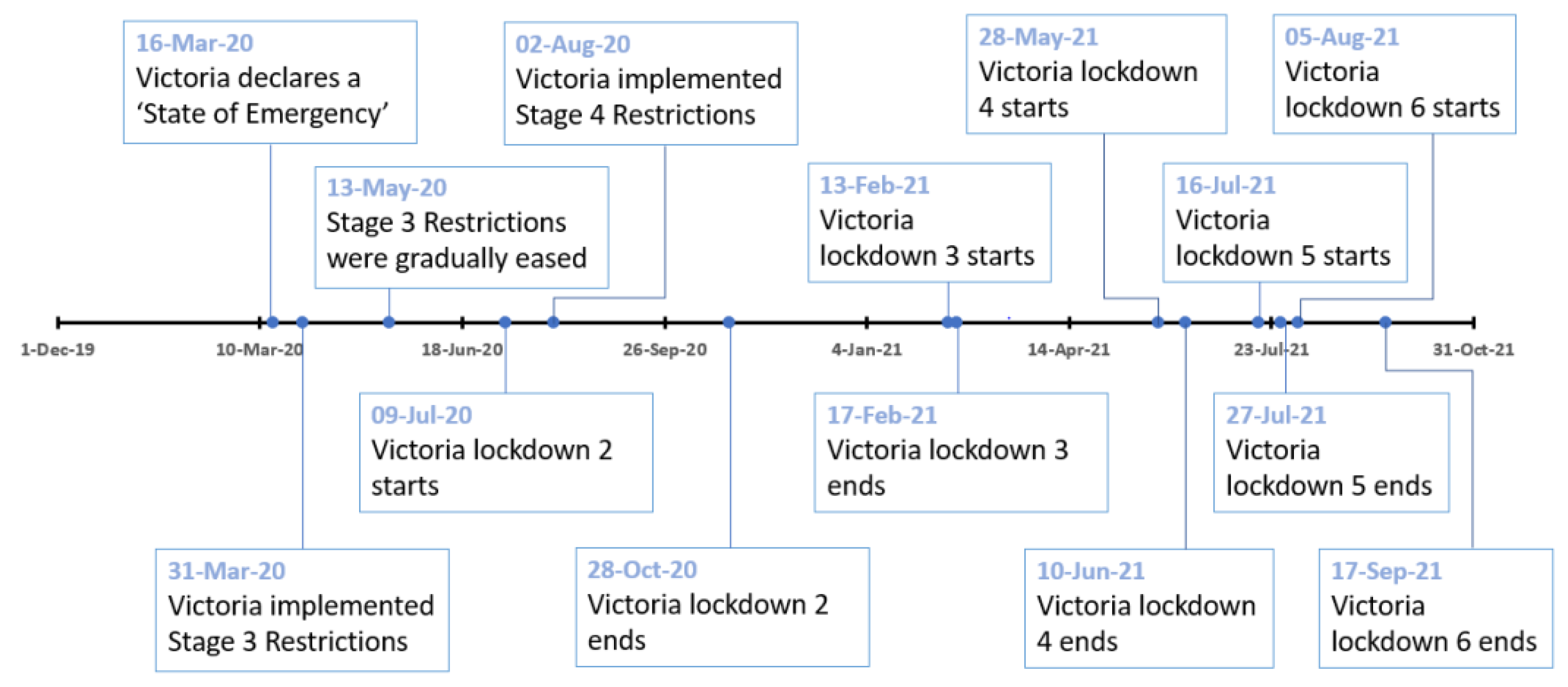
In addition to incorporating data from three commercial buildings at a 15-minute interval, we also integrated the daily COVID-19 case data from the state of Victoria to improve the accuracy of our predictions. During COVID-19, the state of Victoria experienced multiple periods of strict lockdowns and restrictions. The timeline of COVID-19 restriction is shown in Figure 2 [24], and Figure 4 shows the trend of daily COVID-19 cases from February 2020 to January 2021. On March 16, 2020, Victoria declared a “state of emergency,” implementing social distancing measures, work-from-home policies, and restrictions on non-essential activities and travel [25]. Stricter Stage 3 restrictions were introduced on March 31, 2020, which were gradually eased on May 13, 2020, and further relaxed on June 1, 2020.
However, due to a significant rise in COVID-19 cases and breaches in hotel quarantine, Stage 3 restrictions were reintroduced in Metropolitan Melbourne and Mitchell Shire. The second lockdown, known as “Vic lockdown 2,” was announced on July 7, 2020, and scheduled to last for six weeks starting from July 8, 2020 [26]. On August 2, 2020, a state of disaster was declared, and Stage 4 restrictions were implemented in Metropolitan Melbourne for six weeks [27]. This lockdown was later extended to October 28, 2020.
Following an outbreak at the Holiday Inn, Victoria entered a sudden five-day lockdown, known as “Vic lockdown 3,” from February 13, 2021, to February 17, 2021, reverting to Stage 4 restrictions [28]. Lockdown number 4 was another seven-day circuit breaker lockdown that was imposed on May 28, 2021, to combat an outbreak, which was later extended to June 10, 2021 [29]. Victoria then entered a sudden five-day lockdown from July 16, 2021, to July 20, 2021 [28] after the number of Delta cases reached 18. This lockdown was later extended until July 27, 2021 [30]. Just nine days after the easing of restrictions from the fifth lockdown, Victoria entered its sixth lockdown to combat a surge in Delta cases. The announcement was made on August 5, and the lockdown initially lasted for seven days. However, it was later extended until September 17, 2021 [31]. With improvements in the situation, the restrictions were gradually eased, allowing for a return to a semblance of normalcy. However, sporadic outbreaks led to localized lockdowns in different states and territories, with swift and targeted responses to contain the virus. The vaccine rollout gained momentum, offering hope for the future. By late 2021, Australia transitioned from a suppression strategy to living with the virus, adopting a nuanced approach to restrictions and focusing on vaccination rates, setting the stage for post-pandemic recovery.
Figure 2.
Timeline of the Australia COVID-19 pandemic.
3.2. Impact of COVID-19 on Australian Higher Education
Following the World Health Organization’s declaration of COVID-19 as a global pandemic on 11 March 2020, various countries have experienced significant economic, social, and political disruptions. The pandemic has particularly affected countries where universities played a crucial role in the export industry, such as Australia, leading to considerable disruptions and financial challenges for many universities. According to the Department of Education, Skills and Employment (DESE), the total number of international students enrolled in Australian courses in 2021 was 572,349, indicating a 17% decrease compared to the same period in 2020 [32]. The pandemic’s impact on Australian universities is evident through the loss of over 17,000 jobs reported in 2021, as per data from Universities Australia [33]. Even in 2023, the repercussions of the pandemic persist, with universities in Western Australia still suffering financial losses, evident from their 2022 financial reports, which are considerably lower than their figures from 2021 [34]. For Swinburne University of Technology, following a warning issued by the vice-chancellor back in June 2020, [35], the university scrapped more than 100 jobs to address the impacts of COVID-19 on its financial sustainability and declining international student enrollment [36]. Despite the drastic measures, Swinburne University reported a deficit of $48.55 million in its annual report for 2020 [37]. By late 2021, as restrictions were gradually eased in Victoria, Swinburne welcomes international students back to campus [38], and as stated in the 2021 annual report released in 2022, the university finished 2021 with a modest surplus of $11.8 million. This financial result was a good foundation for continued recovery after a disrupted two years, as stated by Vice-Chancellor and President, Professor Pascale Quester [39].
In addition to Energy Consumption in three commercial buildings every 15 minutes, the daily Covid-19 case from its state (i.e.,) Victoria is employed for better forecasting. Australia has faced a series of challenging lockdown measures in response to the COVID-19 pandemic. On March 16, 2020, Victoria declared a “State of Emergency,” urged the public to practice social distancing, avoid non-essential contacts, work from home, and prohibit non-essential gatherings and travel [25]. Subsequently, more rigorous measures were introduced on March 31, 2020, when Victoria implemented Stage 3 Restrictions across the state [28]. Stage 3 Restrictions were gradually eased on May 13, 2020, and further relaxed on June 1, 2020.
Due to a sharp increase in COVID-19 cases and breaches in hotel quarantine, Stage 3 Restrictions were reintroduced in Metropolitan Melbourne and Mitchell Shire. The announcement was made on July 7, 2020, and the second lockdown, known as Vic lockdown 2, was scheduled to last for six weeks starting from July 8, 2020, in order to contain the spread [26]. On August 2, 2020, Victoria declared a State of Disaster, in addition to the existing State of Emergency, and implemented Stage 4 Restrictions in Metropolitan Melbourne for six weeks [27]. However, this lockdown was extended until October 28, 2020. Following an outbreak at the Holiday Inn involving 13 cases of the UK Strain of COVID, Victoria entered a sudden five-day lockdown from February 13, 2021, to February 17, 2021, reverting to Stage 4 Restrictions [28]. On May 28, 2021, Victoria imposed another seven-day circuit breaker lockdown to combat the outbreak, reimposing Stage 4 restrictions and stay-at-home orders reminiscent of the previous lockdowns [29]. The fourth lockdown was extended by seven days and lasted until June 10, 2021. As a result of the Delta variant outbreak in Sydney and the irresponsible actions of interstate delivery drivers from Sydney, Melbourne experienced its own Delta outbreak. When the number of cases in Victoria reached 18, the state entered a sudden five-day lockdown from July 16, 2021, to July 20, 2021 [28]. This lockdown was later extended until July 27, 2021 [30]. Just nine days after the easing of restrictions from the fifth lockdown, Victoria entered its sixth lockdown to combat a surge in Delta cases. The announcement was made on August 5, and the lockdown initially lasted for seven days. However, it was later extended until September 17, 2021 [31].
As the situation improved, restrictions were gradually eased, allowing for a return to a semblance of normalcy. However, sporadic outbreaks led to localized lockdowns in various states and territories, with swift and targeted responses to contain the virus. The vaccine rollout gained momentum, providing hope for the future. By late 2021, Australia began transitioning from a suppression strategy to living with the virus, adopting a more nuanced approach to restrictions, and focusing on vaccination rates, paving the way for a post-pandemic recovery.
4. Methodology
In this section, we describe the proposed model, that is, . An overview of the proposed model is shown in Figure 3. The model aims to forecast the energy used every 15 minutes at commercial buildings during the COVID-19 period. The model has three main phases, namely, data preprocessing, model training, and evaluation. The data preprocessing phase involves the preparation of the input data by applying various preprocessing techniques, such as data differencing, time labeling, data accumulation, and normalization. This step ensures that the data is in a suitable format for further analysis. Next, the model training phase focuses on training the proposed model to capture the complex relationships and dependencies present in the data, enabling accurate predictions. Once the model is trained, the evaluation phase assesses its performance and effectiveness. Various evaluation metrics and techniques are employed to measure the model’s accuracy.
4.1. Data Preprocessing
The data pre-processing phase has two main subphases: (i) processing of the energy consumption and time (ii) and processing of COVID-19 data.
(i) Processing of energy consumption and time. This subphase has 4 steps, (i.e.,) data differencing, time labeling, row concatenation, and widow Slicing. These steps align with the techniques previously introduced by Tan et al. [40]. Data differencing involves calculating the differences between consecutive observations in a time series. The changes between data points are computed instead of using the raw values to make the data stationary. Stationary data is typically easier to model and predict accurately than dynamic data. Peak and non-peak times could reveal underlying trends in the data. Understanding the patterns during these times enables the capture of the variations and the adjustment of the forecasting model accordingly. In this research, 8:00 to 21:00 are referred to as the peak hours, and the others are referred to as the non-peak hours.
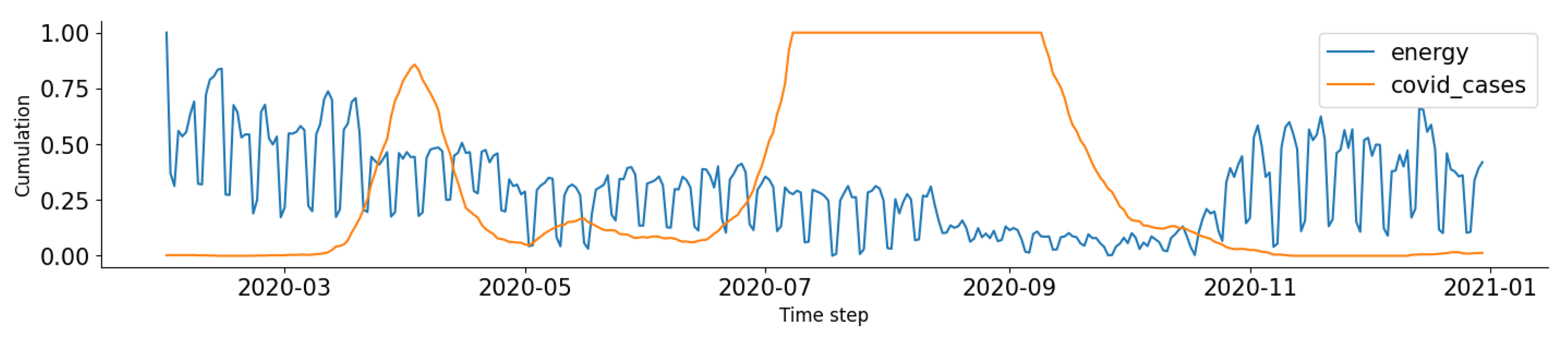
(ii) Processing of the COVID-19 data. During the COVID-19 period, the mobility of people is normally influenced by the number of COVID-19 cases. More restrictions are imposed on people’s movement as the number of COVID-19 cases increases, particularly when accessing commercial buildings. Therefore, the energy consumption in these buildings tends to decrease. Figure 4 illustrates a correlation between the cumulative number of COVID-19 cases in the past 14 days and the corresponding decrease in energy consumption at the Hawthorn Campus - ATC Building. This relationship suggests that as the COVID-19 cases accumulate, a noticeable decline in energy usage occurs within the specified timeframe. The observed trend serves as valuable insight into the impact of COVID-19 on the energy consumption patterns at the mentioned location. Consequently, incorporating this data into forecasting models would be advantageous for accurate predictions. Therefore, two main steps are involved, namely, COVID-19 case cumulation and data normalization. In COVID-19 case cumulation, the cumulative number of COVID-19 cases in the past 14 days is calculated. Then, the data is clipped to 0 to 10,000 range. Clipping helps maintain the data within a reasonable and meaningful range while addressing potential anomalies or extreme values that might skew the model’s behavior. By rescaling the values to this common range, variations in the magnitude of the COVID-19 case counts are eliminated. This normalization process enables fair comparisons between different timesteps and ensures that no single feature dominates the learning process due to its larger magnitude. The normalization formulation is presented in Equation 1.
where represents the cumulation of COVID-19 cases in the previous 14 days for each time step in the 0 to 1 range, and , and are the maximum and minimum COVID-19 cases, respectively.
Figure 4.
Analysis of the trend of daily energy consumption on the basis of the cumulative number of COVID-19 cases over the previous 14 days from February 2020 to January 2021 at the Hawthorn Campus - ATC Building. Note that the cumulation of COVID-19 cases is restricted to the range of 0 to 10,000, and both data are normalized to fit within the range of 0 to 1.
4.2. Forecasting Model
As shown in Figure 3, the proposed model contains two flows of input, namely, (i) energy consumption, and labeled time and (ii) normalized COVID-19 data.
The first input flow focuses on the creation of a specialized multivariate LSTM architecture that is tailored to effectively extract and capture valuable information in the labelled time embedded within the time-series energy consumption. Two consequence LSTM layers exist. LSTM is a type of recurrent neural network (RNN) layer that is specifically designed to capture and model the long-term dependencies and patterns in sequential data [41]. The LSTM layer consists of memory cells that can store and retrieve information over extended sequences. Each memory cell has three main components: an input gate, a forget gate, and an output gate. These gates regulate the flow of information within the LSTM layer.
Within the second input flow, the COVID-19 data is channelled into a dense layer to extract pertinent information that contributes to the overall analysis. This intermediate step helps distil meaningful insights from the COVID-19 data. The resulting output from the dense layer is then combined with the last hidden state of the second LSTM layer, serving as a knowledge injection mechanism. By fusing these two sources of information, the model gains access to both the learned representations from the LSTM layers and the specific COVID-19-related insights. Subsequently, the combination is directed into a series of dense layers and a batch normalization layer positioned in the middle to generate the final decision.
Objective functions are one of the main factors in achieving a high-performing model. Various objective functions are employed for model training. In this research, Huber loss is employed because it is commonly utilized in forecasting tasks due to its robustness against outliers [42] and can strike a balance between the mean absolute error and the mean squared error. This objective function is particularly useful in situations where extreme values may exist, such as in time series forecasting or in datasets affected by anomalous events, like the COVID-19 pandemic. The formulation of Huber loss for each prediction and the corresponding actual value are presented in Equation 2.
where determines the threshold at which the loss function transitions from the quadratic region to the linear region. In this research, the value of is set to 1 for both the proposed and the comparison models employed in this study.
The combination of the proposed data processing techniques and model architecture is designed to ensure robust performance not only during the Covid-19 pandemic but also in similar crisis situations. The models have the potential to accurately capture and forecast key patterns and trends, providing valuable insights and aiding in effective decision-making. The adaptability of the proposed model extends beyond the current pandemic, the model offers a promising solution for accurate forecasting and decision support in the face of further pandemics.
5. Experiment
5.1. Data
This study utilized a dataset comprising energy consumption measurements recorded every 15 minutes in three buildings: the Hawthorn Campus - ATC Building (referred to as ), the Hawthorn Campus - AMDC Building (referred to as ), and the Wantirna Campus - KIOSC Building (referred to as ). Additionally, the dataset includes records of COVID-19 cases in Victoria state in 2020 and 2021.
For all the models, the training set spans from January 2020 to the end of June 2021, while the test set covers the period from July 2020 to the end of December 2021. In the experimental phase, the target variable was predicted based on the 96 immediate previous data points.
5.2. Baseline Model
In this study, we compared the proposed model with four baseline models, namely, linear regression (LR), LSTM, M-LSTM, Bi-LSTM, and SVM.
Linear Regression. LR is a popular statistical model for forecasting. In the context of forecasting, LR aims to establish a linear relationship between the input features and the target variable. The model assumes that this relationship can be represented by a straight line. The goal is to find the best-fitting line that minimizes the difference between the predicted and actual values of the target variable. The model calculates the predicted value of the target variable on the basis of the linear equation, allowing the forecast of future outcomes.
Long Short-term Memory. The LSTM model for forecasting refers to an RNN architecture that consists of a single LSTM layer. This type of model is commonly used to capture temporal dependencies and patterns in sequential data. The energy consumption in the previous sequence of time steps is fed into the LSTM layer, which processes the data over multiple time steps. The LSTM layer contains memory cells that allow the model to retain and utilize the energy information from previous time steps, enabling the capture of long-term dependencies in the data.
Multivariate Multilayered LSTM. In this paper, we compare the proposed model with the M-LSTM model proposed by Tan et al. [40]. The M-LSTM model architecture comprises an input layer, followed by two LSTM layers, and a dense layer at the end. It takes two types of input: energy consumption data recorded every 15 minutes and labelled time information.
Bidirectional Long Short-term Memory. The Bi-LSTM model for forecasting is an RNN architecture that consists of a single Bi-LSTM layer. In this model, the input sequence is bidirectionally processed [43]. The Bi-LSTM layer incorporates both forward and backward LSTMs, allowing the model to simultaneously capture information from past and future time steps. This bidirectional processing enables the model to have a comprehensive understanding of the temporal patterns in the data. The Bi-LSTM model can capture complex temporal dependencies and has been widely employed in various forecasting tasks.
Support Vector Machine. SVM with the radial basis function (RBF) kernel is a popular machine learning model used for forecasting tasks [44]. SVMs are effective in capturing non-linear relationships and have been widely applied in various fields, including time series forecasting. The RBF between two data points (, and ) is presented in Equation 3, with as the parameter that controls the width of the Gaussian curve.
During the training phase, the SVM with RBF kernel adjusts its parameters by solving an optimization problem to find the hyperplane that maximizes the margin and minimizes the errors. This process involves tuning the hyperparameters, such as the kernel parameter () to achieve the best generalization performance.
5.3. Metric
To assess the performance of the model, it is evaluated by generating a set of predictions and comparing them with the corresponding known actual values , where n represents the size of the test set. Three commonly used metrics are employed to measure the overall disparity between these two sets: , , and the R-squared () score. These metrics provide insights into the accuracy and performance of the model’s predictions compared with the actual values.
5.3.1. MAPE
The calculation involves taking the absolute difference between the predicted and actual values, dividing it by the actual value, and then computing the average of these values across the entire dataset, as depicted in Equation 4. This computation yields a single numerical value that represents the average percentage difference between the predicted and actual values. The lower the value is, the better the performance of the model is, because it signifies a smaller average percentage deviation between the predictions and actual values.
5.3.2. NRMSE
The is a performance metric utilized to assess the accuracy of a prediction model. This metric quantifies the normalized average magnitude of the residuals or errors between the predicted and actual values, as indicated in Equation 5. By calculating the square root of the MSEs and normalizing them, the provides a measure of the overall deviation between the predicted and actual values, considering the scale of the data. A low value signifies the good fit of the model to the data, indicating high accuracy in the predictions.
5.3.3. Score
The score, also referred to as the coefficient of determination, is a statistical metric that quantifies the proportion of the variability in the dependent variable that can be explained by the independent variables in a regression model, as depicted in Equation 6. is the mean of the actual values and serves as an indicator of the model’s fitness and its ability to accurately predict the target variable. A high score signifies a good fit of the model, implying that a large portion of the variability in the dependent variable can be accounted for by the independent variables.
5.4. Result
5.4.1. Performance of the Proposed Model on the Training and Test Sets
Figure 5 shows the performance of the proposed model on the training and test sets from three buildings. For , the MPAE, NRMSE, and values are higher for the test set than for the training set by approximately 0.01, 0.03, and 0.03 respectively. For , the MPAE, NRMSE, and are higher for the test set than the test set by approximately 0.03, 0.03, and 0.07 respectively. For , the MPAE, and NRMSE are higher for the test set than the test set by approximately 0.02, and 0.000727344 respectively, and is slightly larger for the test set by approximately 0.02. The MPAE, NRMSE, and values demonstrate a consistent trend across all three datasets, indicating relatively minor discrepancies between the training and test sets.
Figure 6 showcases the forecast generated by the proposed model, specifically for . The outcomes obtained for the remaining datasets follow a similar pattern. The line plot visually demonstrates the model’s fitness and provides a clear representation of how well it aligns with the test set.
In summary, the findings indicate that the proposed model achieves significant optimization when trained on the train set and demonstrates a strong generalization ability when applied to the test set, particularly in the context of the unstable conditions prevailing during the COVID-19 period.
5.4.2. Comparison
Table 2 presents the comparative result of different models on the basis of the following performance metrics: MPAE, NRMSE, and . For , the proposed model demonstrates the best performance, achieving the lowest MPAE (0.061), and NRMSE (0.047) and the highest (0.931). LSTM, Bi-LSTM, and SVM also performed reasonably well, with lower MPAE and NRMSE values than LR. And LR exhibited the highest MPAE and NRMSE values, indicating a larger percentage of error. For , the proposed model maintained its superiority, obtaining lower MPAE and NRMSE values than the other models. Although LSTM, M-LSTM and Bi-LSTM performed relatively well, still exhibited the best accuracy. Finally, for , showcased the best performance with the lowest MPAE and NRMSE values. Despite the relatively higher MPAE and NRMSE values of LSTM and Bi-LSTM, they still outperformed LR and SVM. In particular, LR performed poorly with significantly higher MPAE and NRMSE values and a negative .
To enhance interpretability, instead of showing line graphs at every 15-min interval, we chose to present Figure 7, Figure 8 and Figure 9. These visual representations depict the daily line graphs of the energy consumption forecasts spanning from July 15, 2021 to October 15, 2021 for , , and . The proposed model consistently demonstrated the highest level of accuracy and alignment with the actual data in the three data sets, as illustrated in the figures. Furthermore, the proposed model exhibited greater stability in its predictions, particularly in the challenging context of the COVID-19 period.
In summary, the proposed model consistently outperformed the other models in all three data sets in terms of three metrics. MPAE, NRMSE, and . The model obtained lower MPAE and NRMSE values and higher values than the other models. The results of the proposed model indicate a strong fit and good performance in terms of better capture of the underlying information, especially considering the challenging conditions during the COVID-19 period, which was facilitated by the incorporation of COVID-19 knowledge injection.
6. Conclusion
In summary, this paper presents a novel forecasting model that aims to provide a generic framework that can be adapted to future pandemic scenarios and other comparable crisis situations. As the results obtained from the testing were promising, the proposed model is believed to be sufficient to be applied to any pandemic data. Due to the availability of testing data, the study specifically focused on predicting energy consumption in three buildings located on the Hawthorn and Wantirna campuses. The analysis covers the energy consumption data recorded every 15 minutes during the COVID-19 period from January 2021 to December 2021. Furthermore, the paper proposes a data preprocessing technique tailored to the COVID-19 data, enhancing the understanding of the relationships between the independent variables and the target variables. The results of this study emphasize the notable improvement in performance achieved by the proposed model of energy consumption forecasting with knowledge injection. These findings will play a crucial role in effectively addressing the challenges presented by future pandemics. They should be implemented in energy management systems within commercial buildings to improve building management control and enable more advanced and efficient operations. The experimental results demonstrate that the proposed model, along with the suggested data preprocessing technique, outperforms baseline models including LSTM, Bi-LSTM, LR, and SVM. This superior performance is evident in three widely-used metrics: MPAE, NRMSE, and score. This accomplishment is of significant importance for efficient energy management and conservation within commercial buildings. The practicality of this approach can be extended to other commercial buildings that exhibit similar energy consumption patterns, rendering it a feasible solution for energy management in this sector. Additional investigation could focus on evaluating the efficacy of the suggested pre-processing method and models in forecasting energy consumption across diverse building types or larger datasets. Exploring alternative techniques, like seasonal decomposition or time series analysis, to incorporate temporal information into the models may yield valuable findings. Further expansion of the research can involve incorporating a 24-hour-ahead electrical load forecast, which can be used as day-ahead electrical load information. In addition to the inclusion of additional input features, such as occupancy and equipment-level information (e.g., the thermostat setpoint, the brightness of the lighting system, and the number of devices connected to plug loads), historical load data and weather information can be included to enhance the accuracy of electrical load forecasting. These advances in energy consumption forecasting have the potential to generate substantial cost savings and environmental advantages, particularly within commercial buildings.
References
- Year-on-year change in weekly electricity demand, weather corrected, in selected countries, January- December 2020 – Charts – Data Statistics - IEA — iea.org. (https://www.iea.org/data-and-statistics/charts/year-on-year-change-in-weekly-electricity-demand-weather-corrected-in-selected-countries-january-december-2020?fbclid=IwAR0dN3dOAKFw85WuJr0bFJyTeOseC6U9kWfVSSuWZZT8I3sQUAkVdC2tQ), Accessed 03 Jul 2023.
- I. H. Panhwar, K. Ahmed, M. Seyedmahmoudian, A. Stojcevski, B. Horan, S. Mekhilef, A. Aslam, and M. Asghar. Mitigating power fluctuations for energy storage in wind energy conversion system using supercapacitors. IEEE Access. 8 pp. 189, 747–189, 760 (2020). [CrossRef]
- G. S. Thirunavukkarasu, M. Seyedmahmoudian, E. Jamei, B. Horan, S. Mekhilef, and A. Stojcevski. Role of optimization techniques in microgrid energy management systems—a review. Energy Strategy Reviews. 43 p. 100899 (2022). [CrossRef]
- Australian Bureau of Statistics 2023, Energy Account, Australia, Australian Bureau of Statistics 2023. (https://www.aer.gov.au/wholesale-markets/wholesale-statistics/annual-generation-capacity-and-peak-demand-nem), Accessed 17 May 2023.
- Santiago, I., Moreno-Munoz, A., Quintero-Jiménez, P., Garcia-Torres, F. & Gonzalez-Redondo, M. Electricity demand during pandemic times: The case of the COVID-19 in Spain. Energy Policy. 148 pp. 111964 (2021). [CrossRef]
- Alasali, F., Nusair, K., Alhmoud, L. & Zarour, E. Impact of the COVID-19 Pandemic on Electricity Demand and Load Forecasting. Sustainability. 13 (2021). [CrossRef]
- Zhong, H., Tan, Z., He, Y., Xie, L. & Kang, C. Implications of COVID-19 for the electricity industry: A comprehensive review. CSEE Journal Of Power And Energy Systems. 6, 489-495 (2020). [CrossRef]
- Sinden, G. Characteristics of the UK wind resource: Long-term patterns and relationship to electricity demand. Energy Policy. 35, 112-127 (2007).
- Rosenberg, E., Lind, A. & Espegren, K. The impact of future energy demand on renewable energy production – Case of Norway. Energy. 61 pp. 419-431 (2013). [CrossRef]
- Norouzi, N., Zarazua de Rubens, G., Choupanpiesheh, S. & Enevoldsen, P. When pandemics impact economies and climate change: Exploring the impacts of COVID-19 on oil and electricity demand in China. Energy Research & Social Science. 68 pp. 101654 (2020).
- Bedi, J. & Toshniwal, D. Deep learning framework to forecast electricity demand. Applied Energy. 238 pp. 1312-1326 (2019). [CrossRef]
- Klemeš, J., Fan, Y. & Jiang, P. The energy and environmental footprints of COVID-19 fighting measures – PPE, disinfection, supply chains. Energy. 211 pp. 118701 (2020). [CrossRef]
- Lu, H., Ma, X. & Ma, M. A hybrid multi-objective optimizer-based model for daily electricity demand prediction considering COVID-19. Energy. 219 pp. 119568 (2021). [CrossRef]
- Haque, A. & Rahman, S. Short-term electrical load forecasting through heuristic configuration of regularized deep neural network. Applied Soft Computing. 122 pp. 108877 (2022). [CrossRef]
- Gómez-Omella, M., Esnaola-Gonzalez, I., Ferreiro, S. & Sierra, B. k-Nearest patterns for electrical demand forecasting in residential and small commercial buildings. Energy And Buildings. 253 pp. 111396 (2021). [CrossRef]
- Brucke, K., Arens, S., Telle, J., Steens, T., Hanke, B., Maydell, K. & Agert, C. A non-intrusive load monitoring approach for very short-term power predictions in commercial buildings. Applied Energy. 292 pp. 116860 (2021). [CrossRef]
- Zhou, D., Ma, S., Hao, J., Han, D., Huang, D., Yan, S. & Li, T. An electricity load forecasting model for Integrated Energy System based on BiGAN and transfer learning. Energy Reports. 6 pp. 3446-3461 (2020). [CrossRef]
- Ngo, N., Truong, T., Truong, N., Pham, A., Huynh, N., Pham, T. & Pham, V. Proposing a hybrid metaheuristic optimization algorithm and machine learning model for energy use forecast in non-residential buildings. Scientific Reports. 12, 1065 (2022). [CrossRef]
- Ibrahim, B. & Rabelo, L. A deep learning approach for peak load forecasting: A case study on panama. Energies. 14, 3039 (2021). [CrossRef]
- Huang, Y., Hasan, N., Deng, C. & Bao, Y. Multivariate empirical mode decomposition based hybrid model for day-ahead peak load forecasting. Energy. 239 pp. 122245 (2022). [CrossRef]
- Yin, L. & Xie, J. Multi-temporal-spatial-scale temporal convolution network for short-term load forecasting of power systems. Applied Energy. 283 pp. 116328 (2021). [CrossRef]
- Wu, D., Hur, K. & Xiao, Z. A GAN-enhanced ensemble model for energy consumption forecasting in large commercial buildings. IEEE Access. 9 pp. 158820-158830 (2021). [CrossRef]
- Ishaq, M., Kwon, S. & Others Short-term energy forecasting framework using an ensemble deep learning approach. IEEE Access. 9 pp. 94262-94271 (2021). [CrossRef]
- Timeline of Every Victoria Lockdown (Dates & Restrictions), bigaustraliabucketlist 2021. (https://bigaustraliabucketlist.com/victoria-lockdowns-dates-restrictions/), Accessed 17 May 2023.
- State Of Emergency Declared In Victoria Over COVID-19, Premier of Victoria 2020. (https://www.premier.vic.gov.au/state-emergency-declared-victoria-over-covid-19), Accessed 17 May 2023.
- COVID-19 Update | 7 July 2020, National Retail Association 2020. (https://www.nra.net.au/covid-19-update-7-july-2020).
- Coronavirus: What changes under Melbourne’s Stage 4 restrictions, 9NEWS 2020. (https://www.9news.com.au/national/coronavirus-melbourne-stage-4-restrictions-explained-curfews-lockdown-what-is-open-closed-changes-covid19/652ee0f9-cc22-41df-b465-9a765a45c496), Accessed 17 May 2023.
- Statement From The Premier, Premier of Victoria 2021. (https://www.premier.vic.gov.au/statement-premier-92), Accessed 17 May 2023.
- COVID LOCKDOWN: Victoria announces major restrictions to combat coronavirus outbreak, 7NEWS 2021. (https://7news.com.au/lifestyle/health-wellbeing/covid-lockdown-victoria-announces-major-restrictions-to-combat-coronavirus-outbreak-c-2148043), Accessed 17 May 2023.
- Extended Lockdown And Stronger Borders To Keep Us Safe, Premier of Victoria 2021. (https://www.premier.vic.gov.au/extended-lockdown-and-stronger-borders-keep-us-safe), Accessed 17 May 2023.
- Seven Day Lockdown To Keep Victorians Safe, Premier of Victoria 2021. (https://www.premier.vic.gov.au/seven-day-lockdown-keep-victorians-safe), Accessed 17 May 2023.
- International student numbers by country, by state and territory. (https://www.education.gov.au/international-education-data-and-research/international-student-numbers-country-state-and-territory), Accessed: 2023-02-07.
- More than 17,000 jobs lost at Australian universities during Covid pandemic. (https://www.theguardian.com/australia-news/2021/feb/03/more-than-17000-jobs-lost-at-australian-universities-during-covid-pandemic), Accessed: 2023-02-07.
- WA universities lose millions as COVID’s bite continues to be felt. (https://www.watoday.com.au/national/ western-australia/wa-universities-lose-millions-as-covid-s-bite-continues-to-be-felt-20230329-p5cwe5. html), Accessed: 2023-02-07.
- Swinburne staff warned of job cuts as universities’ COVID-19 woes grow. (https://www.theage.com.au/ national/victoria/swinburne-staff-warned-of-job-cuts-as-universities-covid-19-woes-grow-20200603- p54z6s.html), Accessed: 2023-02-07.
- Swinburne University staff condemn leadership over ’excessive’ cuts to courses, jobs. (https://www.theage.com.au/national/victoria/swinburne-university-staff-condemn-leadership-over-excessive-cuts-to-courses-jobs-20201112-p56dyy.html), Accessed: 2023-02-07.
- RMIT, Swinburne, La Trobe post hefty deficits but not all unis in the red. (https://www.theage.com.au/national/victoria/rmit-swinburne-la-trobe-post-hefty-deficits-but-not-all-unis-in-the-red-20210504-p57ova.html), Accessed: 2023-02-07.
- Swinburne welcomes international students back to campus. (https://www.swinburne.edu.au/news/2021/11/swinburne-welcomes-international-students-back-to-campus/), Accessed: 2023-02-07.
- Swinburne’s strategic focus delivers financial turnaround – 2021 Annual Report released. (https://www.swinburne.edu.au/news/2022/05/swinburnes-strategic-focus-delivers-financial-turnaround-2021-annual-report-released/), Accessed: 2023-02-07.
- Dinh, T., Thirunavukkarasu, G., Seyedmahmoudian, M., Mekhilef, S. & Stojcevski, A. Predicting Commercial Building Energy Consumption Using a Multivariate Multilayered Long-Short Term Memory Time-Series Model. Applied Sciences. (2023).
- Hochreiter, S. & Schmidhuber, J. Long short-term memory. Neural Computation. 9, 1735-1780 (1997).
- Huang, S. Robust learning of Huber loss under weak conditional moment. Neurocomputing. 507 pp. 191-198 (2022).
- Schuster, M. & Paliwal, K. Bidirectional recurrent neural networks. Signal Processing, IEEE Transactions On. 45 pp. 2673 - 2681 (1997,12) https://www.mdpi.com/2071-1050/13/3/1435.
- Liu, Z., Wu, D., Liu, Y., Han, Z., Lun, L., Gao, J., Jin, G. & Cao, G. Accuracy analyses and model comparison of machine learning adopted in building energy consumption prediction. Energy Exploration & Exploitation. 37 (2019,1).
Figure 1.
Statistics of final energy consumption by end-users in Australia from 2016 to 2021 [4].
Figure 1.
Statistics of final energy consumption by end-users in Australia from 2016 to 2021 [4].
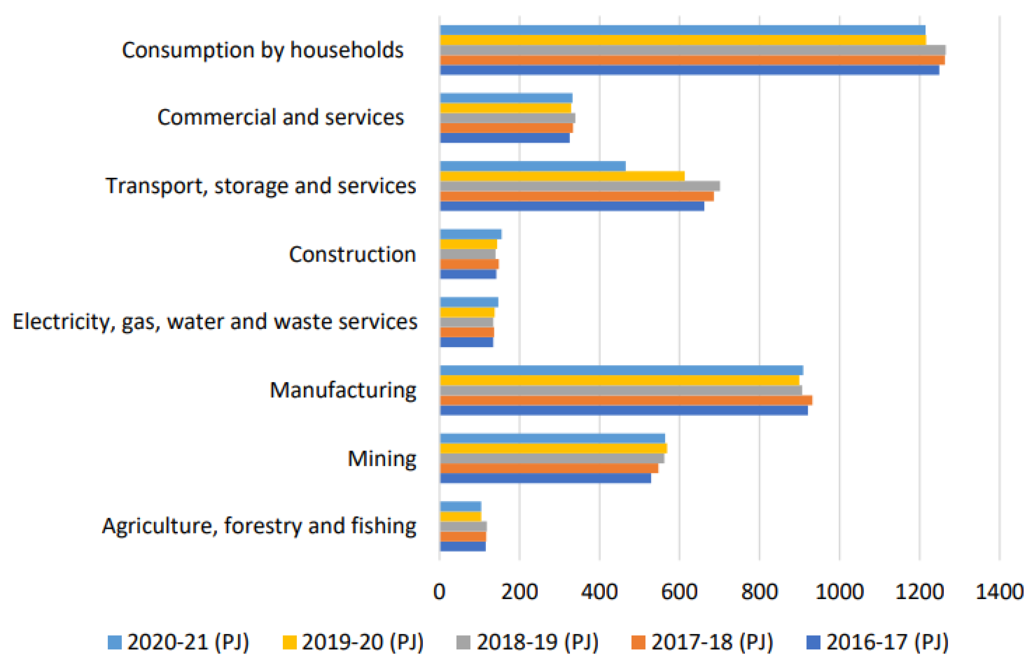
Figure 3.
Overview of the proposed model.
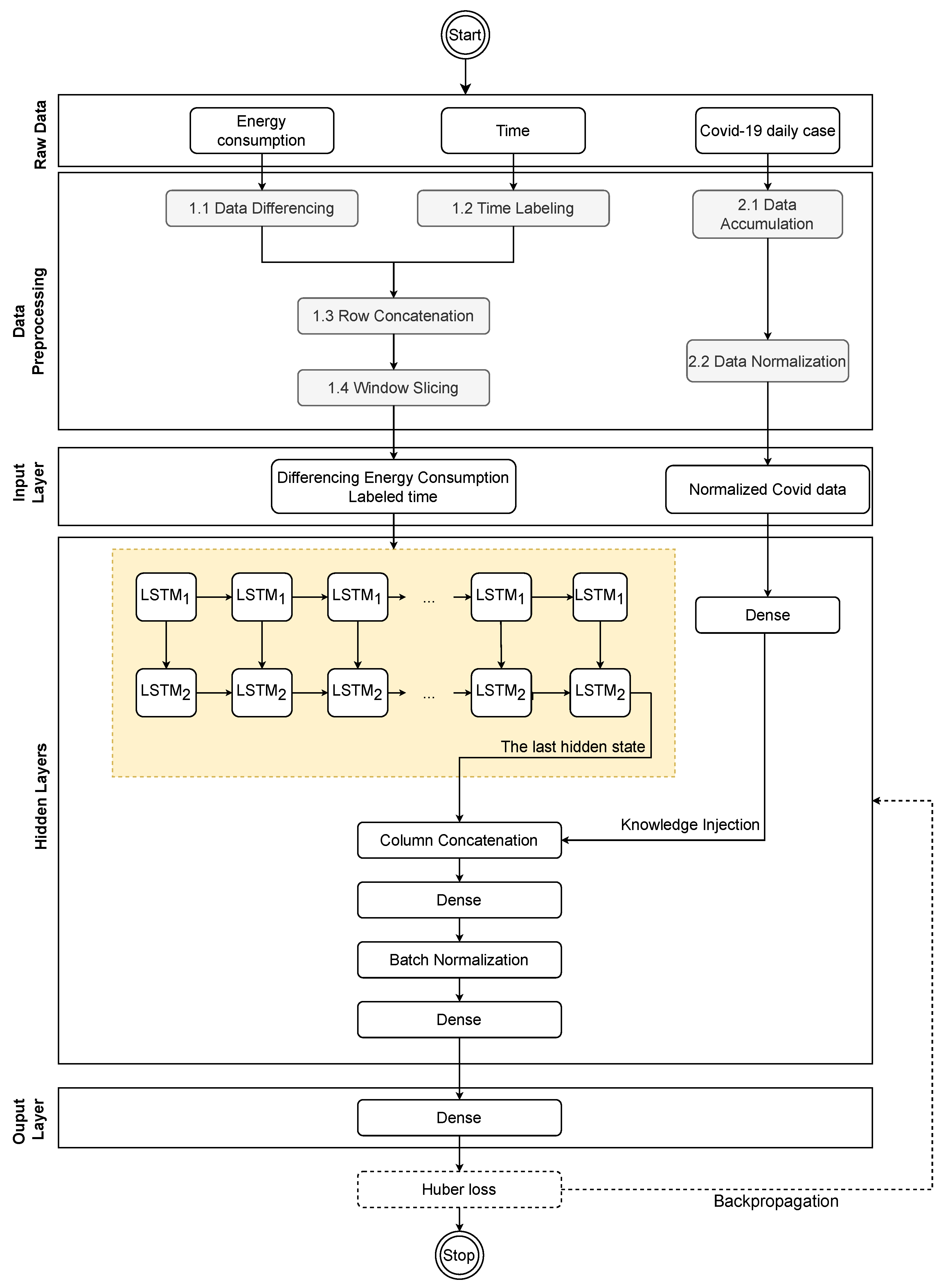
Figure 5.
Performance of the proposed model on training and test sets in terms of three metrics: MPAE, NRMSE, and (or R2 as shown in image), in three datasets: (a) , (b) , (c) .
Figure 5.
Performance of the proposed model on training and test sets in terms of three metrics: MPAE, NRMSE, and (or R2 as shown in image), in three datasets: (a) , (b) , (c) .
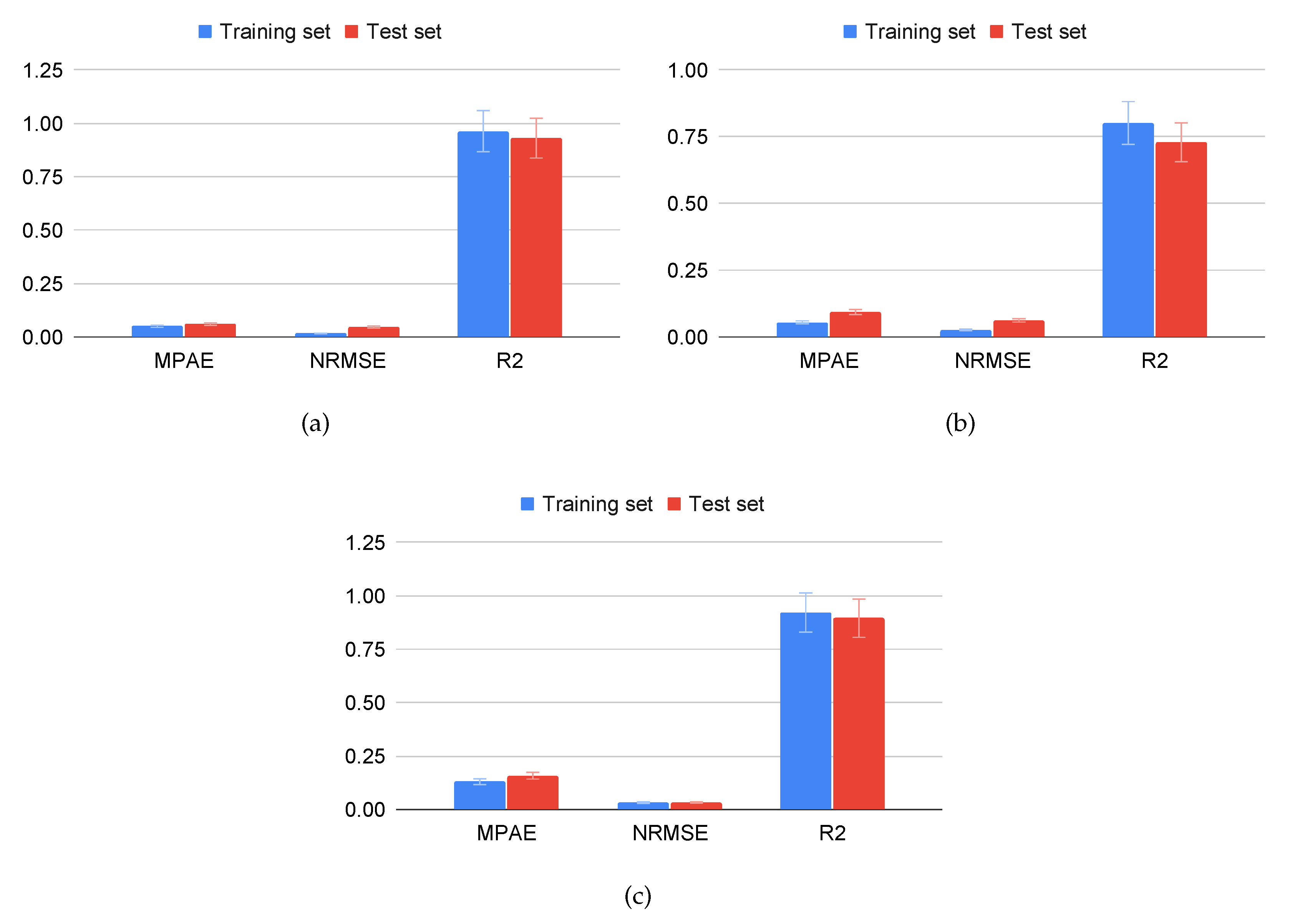
Figure 6.
Prediction of the proposed model on from July 15, 2021, to January 1, 2022, every 15 minutes with a step size of 96.
Figure 6.
Prediction of the proposed model on from July 15, 2021, to January 1, 2022, every 15 minutes with a step size of 96.
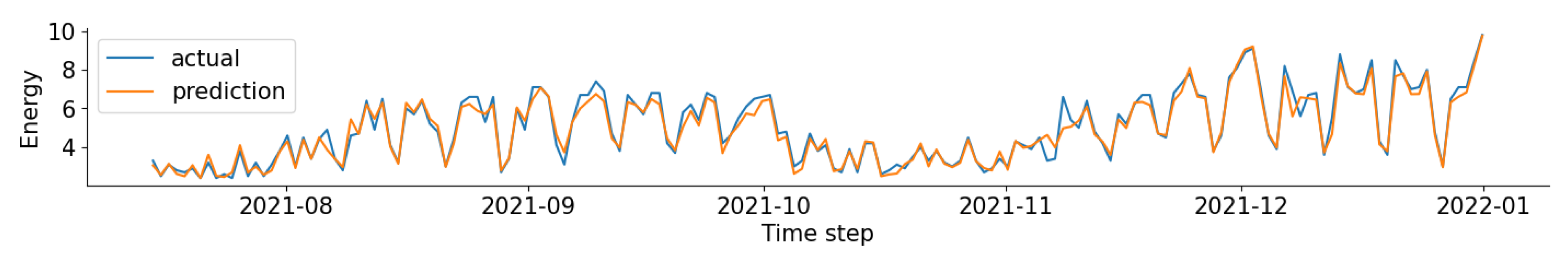
Figure 7.
Prediction for energy consumption every day of forecasting models on
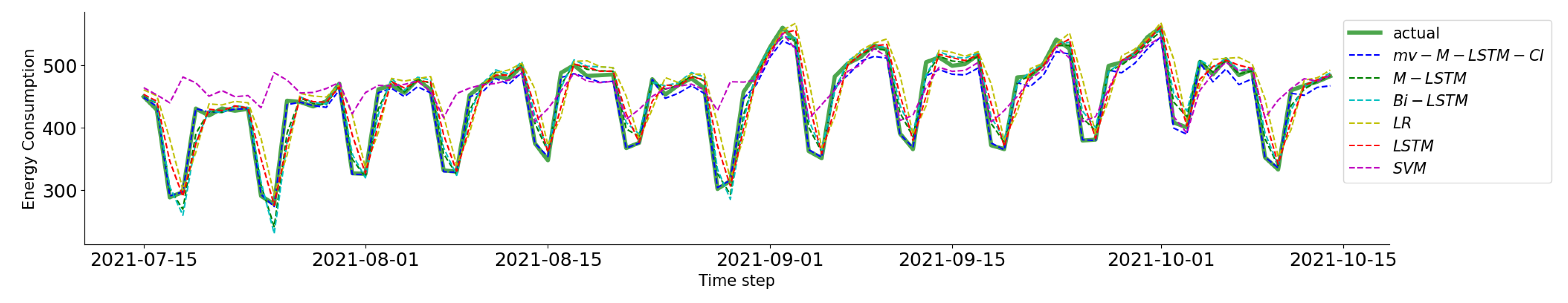
Figure 8.
Prediction for energy consumption every day of forecasting models on
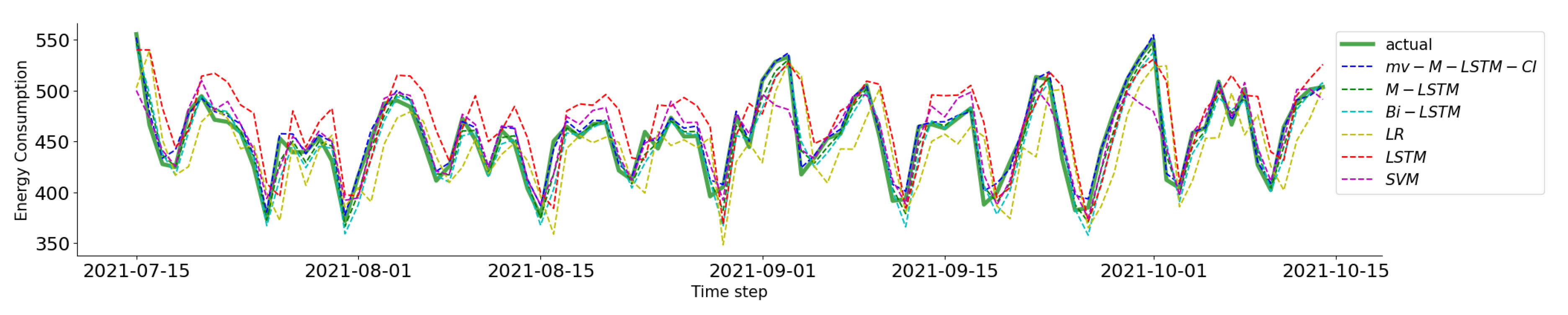
Figure 9.
Prediction for energy consumption every day of forecasting models on
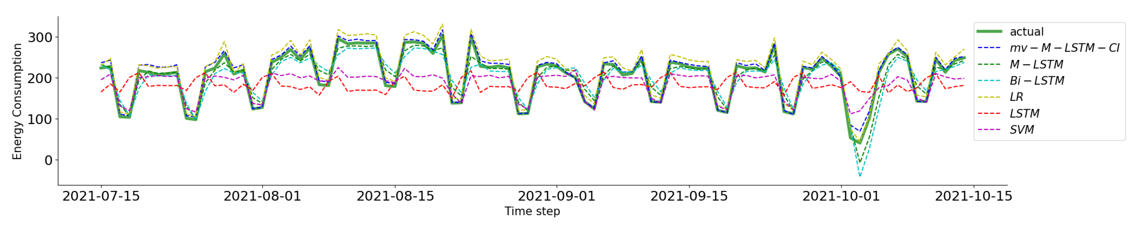
Table 2.
Comparison of forecasting models in terms of three metrics on three datasets. The best values are marked in bold.
Table 2.
Comparison of forecasting models in terms of three metrics on three datasets. The best values are marked in bold.
| Dataset | Model | Metric | ||
|---|---|---|---|---|
| MPAE | NRMSE | |||
| 0.061 | 0.047 | 0.931 | ||
| LSTM | 0.366 | 0.100 | 0.690 | |
| M-LSTM | 0.103 | 0.094 | 0.784 | |
| Bi-LSTM | 0.365 | 0.088 | 0.760 | |
| LR | 0.396 | 0.143 | 0.365 | |
| SVM | 0.179 | 0.108 | 0.638 | |
| 0.093 | 0.062 | 0.729 | ||
| LSTM | 0.204 | 0.098 | 0.323 | |
| M-LSTM | 0.098 | 0.123 | 0.391 | |
| Bi-LSTM | 0.211 | 0.077 | 0.588 | |
| LR | 0.270 | 0.196 | -0.699 | |
| SVM | 0.131 | 0.101 | 0.286 | |
| 0.158 | 0.033 | 0.895 | ||
| LSTM | 0.802 | 0.085 | 0.298 | |
| M-LSTM | 0.711 | 0.105 | 0.676 | |
| Bi-LSTM | 0.946 | 0.064 | 0.603 | |
| LR | 0.926 | 0.110 | -0.169 | |
| SVM | 0.389 | 0.068 | 0.550 | |
Disclaimer/Publisher’s Note: The statements, opinions and data contained in all publications are solely those of the individual author(s) and contributor(s) and not of MDPI and/or the editor(s). MDPI and/or the editor(s) disclaim responsibility for any injury to people or property resulting from any ideas, methods, instructions or products referred to in the content. |
© 2023 by the authors. Licensee MDPI, Basel, Switzerland. This article is an open access article distributed under the terms and conditions of the Creative Commons Attribution (CC BY) license (http://creativecommons.org/licenses/by/4.0/).
Copyright: This open access article is published under a Creative Commons CC BY 4.0 license, which permit the free download, distribution, and reuse, provided that the author and preprint are cited in any reuse.


