
Submitted:
22 July 2023
Posted:
24 July 2023
Read the latest preprint version here
Abstract
Solar geoengineering (SG) solutions have many advantages compared to the difficulty of carbon removal (CR): SG produces fast results, is shown here to have much higher efficiency than CR, is not related to fossil fuel legislation, and is something we all can participate in brightening the Earth with cool roofs, and roads. SG requirements detailed previously to mitigate global warming (GW) have been concerning primarily because of overwhelming goals and climate circulation issues. In this paper, higher feasibility is provided for solar geoengineering applications by focusing on physics-based estimates to stop annual increases in GW. Annual solar geoengineering (ASG) area modification requirements found here are generally 50 to possibly higher than 150 times less compared to the challenge of full SG GW mitigation. Results indicate that AI paint drone technology is likely needed for Earth brightening to meet annual mitigation goals. As well, results indicate much higher feasibility for L1 space shading compared to prior literature estimates for full GW mitigation. However, stratosphere injections appear challenging in the annual approach. A serious issue with implementing ASG is the problem of worldwide negative SG which currently dominates yearly practices with the application of dark asphalt roads and roofs. This issue is discussed.
Keywords:
Solar geoengineering
; Modeling
; Space Mirrors
; Earth Mirrors
; Desert Modification
; Space Clusters
; Stratosphere Injection
1. Introduction
This paper provides fundamental physics-based annual solar geoengineering (ASG) equations to aid in estimated requirements for yearly area solar radiation modification (SRM). Therefore, this paper provides initial assessments without using computer-aided full climate solutions. Solar geoengineering physics should add a deeper understanding of annual requirements. Estimates are simplified by focusing on temperature which is the key thermodynamic driver for the climate system and ASG.
The IPCC worries about an increase of a 1.5oC rise over the pre-industrial period. This is estimated to possibly occur around 2039-2043 at the current rate of yearly temperature increases. This can be estimated from Figure 1 which shows the short-term GW trends occurring around 2052. However, the graph displays changes since 1975. The IPCC warning is referenced to the pre-industrial period. Translating Figure 1 to the pre-industrial period requires adding about 0.17oC. Then this would occur around 2043 from the graph.
ASG will require timely yearly construction rate reflective modified areas both on Earth and possibly in space to reduce some of the Sun’s energy to mitigate yearly global warming increases. Thus, a key purpose of ASG is to maintain the status quo allowing time for future mitigation improvements and because goals are limited to mitigating yearly warming increases, many controversial SG issues are minimized.
From the graph’s equation, the current rate of global warming is an increase in temperature of 0.019oC/year. To maintain the status quo for zero global warming growth, we can divide up the ASG construction task into two parts for simplicity. Half relegated to the stratosphere (Sec. 3.4) or space shading methods. Half relegated to land-based solutions such as that proposed by project MEER [1] but on a larger scale (see Sec 3.4). Therefore, a reasonable goal is to mitigate a 0.019oC/year global warming increase which should minimize circulation concerns [2,3,4,5] and many other controversial issues. This goal turns out to be about 50 to possibly higher than 150 times less mitigation in Earth brightening area modification requirements compared to prior full mitigation estimates [6].
Most of the current SRM literature is focused on stratosphere aerosol injections (SAI). As this is covered by computer-aided models and there are a lot of concerns in this area, this paper focuses more on Earth-brightening and L1 space Sun dimming solutions. However, we do overview some of the physics that may be helpful for SAI. There are many reasons that SAI may not be appropriate for ASG. The primary one is yearly maintenance needs [2,3,4,5]. This is less of a problem in SRM methods like Earth-brightening. For example, negative SRM appears well maintained in the area of asphalt roads and roofs This negative example, illustrates the low maintenance requirements that could occur with Earth-brightening modifications. Negative solar geoengineering is a worldwide problem and impedes opportunities for positive SG advances. This needs to be addressed and is discussed in Sec. 4.4.
2. Method and Data
2.1. Zero global warming growth
In this paper, the approach is to provide basic physics-based estimates to achieve just enough solar geoengineering to reverse the potential yearly increase in global warming. In this paper, this is referred to as annual solar geoengineering. For example, global warming from 1975 to 2022 was 0.9oC [7]. If a status quo annual solar geoengineering approach was applied, the ideal result would be a zero temperature increase. The warming level would stay at 0.9oC. According to Figure 1, the current temperature reversal requirement for ZGWG is
TR=-0.0188oC/year
2.2. Theory
In this section, the basic physics-based ASG goals are presented. The numbers used in this section and Sec. 3 can be updated for more complex computer-aided models depending on the reader’s interest and the changing climate. As well, we mostly use averages in approximating estimates. The estimated general requirements to offset a temperature increase in energy units is
TR=-0.0188oC/year=-0.102Wm-2/year
This conversion to energy units can be obtained from the Stephan-Boltzmann relation where
Here T1 is taken as the average surface temperature of the Earth of about 14.5oC and T2=14.5 oC+0.0188oC=14.519oC.
The SG strategy developed by the author [6] indicates to reverse the global warming that occurred from 1950 to 2019 having a temperature rise of 0.95oC, would require a reversal of. This is just the global warming rise from 1950 to
2019 of 0.95oC in energy units where . Here 287.65K=14.5oC is roughly the average temperature of the Earth. Then we can write for full global warming mitigation (from 1950 to 2019) from the author’s prior work [6], the reversal equates to
In this equation, the reverse forcing due to an albedo
change of the target is denoted by. We note that increasing the reflectivity of a hotspot surface reduces its associated greenhouse gas effect This is estimated in Eq. 4 with the 1+f term where f is approximately 0.62 [8]. This is due to the average re-radiation estimate of 62% [8]. In this equation, we assume that feedback, which is dominated by water vapor, will also reverse. That is, SG reverse forcing causes a cooling effect and cooler air holds less water vapor. In Eq. 4, the average feedback value is estimated in 2019 as [8,9]. We note that many other authors have anticipated a similar feedback-doubling effect [10,11]. However, this value can be written with temperature dependence, and this is discussed in Sec. 2.3.
Then inserting into Eq. 4, we can write
This is the estimated goal for a total reversal of global warming from 1950 to 2021. Other updated estimates may be used depending on the reader’s interest. Since in this paper, we are interested in zero global warming annual growth, the ASG requirement for a reversal is approximated as (from Eq. 3-5)
This is the estimated main reverse forcing results used in this paper.
2.2.1. Greenhouse gas equivalent reduction from SRM
It is helpful to note the SG advantage in Eq. 5. To mitigate the 5.1Wm-2 in Eq. 4, requires an estimated SG change of -1.47Wm-2 compared to trying to do it with GHG removal which would require the full 2.38Wm-2. This yields a work savings of 0.91Wm-2 (=2.38Wm-2-1.47Wm-2). This is a 38% (=0.91Wm-2 /2.38Wm-2) SG advantage [8] yielding much higher efficiency compared to CR. That is in SG, we need to take into account a 1+f re-radiation extra reduction in Eq. 5, (i.e., increasing the reflectivity of a hotspot surface additionally reduces its associated greenhouse gas effect [8]).
Therefore, by cooling a hotspot, we effectively reduce its GHG effect. Essentially, if we did full GW mitigation of the increases from 1950 to 2019 using SRM, we would reduce effectively 0.91Wm-2 of the associated GHG effect. Many authors do not consider this SG ‘effective GHG reduction’. Yet, on average, an additional 62% of SRM goes into its associated “GHG equivalent reduction’.
This GHG-albedo effect may also help to decrease the high levels of possible CO2 and often water vapor feedback re-radiation that can occur in UHIs in the presence of high heat flux [12,13].
Unfortunately, alternately worldwide negative solar geoengineering equivalently increases the GHG effect by this 1+f factor (Sec. 4.4), and its additional associated water vapor feedback increases. When these average effects are considered in addition to the background climate, urbanization heat fluxes from impermeable surfaces are problematic on both the local and global levels [13,14] as discussed in Sec. 4.4.
2.2.2. Area estimates for annual solar geoengineering
To estimate the Eq. 6 area modification requirements for a -0.0293Wm-2 reversal, the approach is to use the author’s derived solar geoengineering estimate [6] that is given by
This physics-based SG equation indicates that in Earth brightening, as anticipated, the reversal is proportional to the target area AT, the amount of irradiance Xc falling on the target with global averages of 47% [15], and the average solar energy over 24 hours,. In addition, the albedo change is, where the target’s albedo changes from to its SG increase.
Note that a space irradiance factor XS has been introduced, and is generally taken as unity. However, for space mirror application, the optimal L1 point rotates around the Sun with the same angular speed as the Earth, thus allowing constant shading. Then the irradiance shading occurs 24 hours a day and the Earth’s curvature is not a factor. This increases So/4 to So. To account for the increase in space irradiance, we can let XS=4 in Eq. 7.
This equation also provides provisions for targets in urban heat island (UHI) areas which can have microclimate de-amplification effects denoted by HT [13,16]. For example, in UHIs, the solar canyon effect amplifies warming when buildings reflect light onto pavements amplifying heat at the surface. Other amplification issues can include re-radiation due to the increase in local CO2 GHGs, local water vapor feedback, temperature inversions, loss of wind and evapotranspiration cooling, increases in solar heating of impermeable surfaces from building sides, pavements heat fluxes, and so forth [13]. Some of these effects will reverse and de-amplify, increasing cooling, and can be accounted for in Eq. 7 with the HT variable. City heat flux amplification is often observed by the UHI’s dome and footprint. The footprint and dome growth are indications of amplified heat flux that is observed to spread beyond the boundaries of the city itself both horizontally and vertically [13,16].
2.3. The Potential Advantage in Earth Brightening of Hotspots
In terms of an albedo change, it is clear from Eq. 4, the larger the albedo change, the smaller the required target area that is needed to meet a specific SG goal. However, the impact of different albedo changes, according to Equations 4 and 5, creates the same average water vapor feedback effect. Therefore, we would like to assess the effect of cooling a high-temperature hotpot surface by considering its feedback temperature dependence rather than using an average factor. We later define a hotspot area below.
To look at hotspot issues, consider the Clausius-Clapeyron relation. To assess this potential effect, Eq. 4 can be written with temperature dependence
The rule of thumb is a decrease in water vapor goes as the temperature ratio. However, the most accurate method is to use the Clausius-Clapeyron humidity relationship between two temperature changes as
Here T1 and T2 are in degrees K, 2.465E6 J-kg−1 is the latent heat of vaporization and 462 J-kg−1 K−1 is the specific gas constant for water vapor, and we can denote the Clausius-Clapeyron humidity relationship by CC.
For example, if we take the average temperature of the Earth as 14.5oC, the estimated AF factor at 27oC is
This is close to the average . It is estimated that water vapor feedback is dominated
by tropical areas [10,11] where an average temperature
of 27oC would be reasonable. This provides a helpful point estimate for
the average value .
Consider an effort to do Earth brightening focusing solely on hotspot areas. As an example, consider a hotspot asphalt surface area averaging 61oC that is changed to a cool road close to the region’s ambient which in this example we take as 33oC. Then the Clausius-Clapeyron relation indicates the potential for a local region cooling to reduce its water vapor effect and how it could change its feedback factor. Then the potential feedback factor could effectively increase to
Compared to, the local value is doubled to. Then according to Equations 4 and 5, Eq. 6 local goal
would be cut in half where
This feedback is related to thermal equilibrium and how it can factor into reducing water vapor content in the atmosphere and its potential local re-radiation effect. Therefore, these are potential estimates and likely maximum assessments. A full computer climate model may provide more insight. This is simply an example to help illustrate the importance of hotspot cooling and its potential water vapor feedback effect. Note in comparison to Eq. 5, ASG in this case is a factor of 100 times reduced. Section 3.4 summarizes this maximum hotspot cooling potential results. Sec. 3.1 illustrates the potential full advantage of selecting hotspot targets for cooling and the importance of being able to cool T2 where T2 >> T1. We might then define a hotspot as having the potential in which AF(T) is reasonably greater than the estimated average .
Note that a factor of two higher (Eq. 11) is not unreasonable for an urban heat island water vapor feedback compared to the standard atmosphere. Zhao et al. [17] compared similarly constructed cities with twenty-four located in the humid southeastern United States to 15 cities in dry climates. They found an average ΔT increase of 3.3 K observed in daytime hours in humid climates with little differences in nighttime hours. Feinberg [12] modeled UHI water vapor feedback based on Zhao et al.’s [17] data set. The mathematical treatment found a UHI local feedback value of 3.4 Wm−2 K−1 [12] for cities in humid environments at 15 °C. This is about a factor of 2.1 higher compared to some authors’ estimates for average feedback in the standard atmosphere [11].
Again on the flip side, we note the potential water vapor feedback increases are likely associated with worldwide negative solar geoengineering (Sec. 4.4).
3. Results
3.1. Cool pavement model estimate
As an example, consider the required area for worldwide cool pavements. We can consider an average asphalt pavement albedo of about, and using cool road methods, estimate an increase
for the pavement albedo of . Then considering an average irradiance of , with , , and , and using a 50% ASG reversal goal, the requirement
is
Solving we obtain the SG target area percentage for half of ZGWG yielding an area modification of
The pavement modification area that needs to be cooled for a change equates to
This yields an equivalent radius of 138 miles. This result is summarized in Section 3.4. This is simply an example to provide estimated area modification requirements. Other values may be used depending on the reader’s interest.
For pavements that are cooled with (see Sec. 2.3), the requirement for the area modification
is much less according to Sec. 2.3. In this case it is likely that . Letting for this example, the area modification is reduced
to
This yields a reduced equivalent radius of 76 miles. This result is also summarized in Sec. 3.4. Note that to achieve these results; the goal for 50% mitigation is reduced by more than half.
If we could do full global warming SG mitigation for per the equivalent cool pavements in Eq. 15 but with ,, , the area required would be about 6 million square
miles. In comparison, this ASG requirement where , , and hotspot mitigation with, the resulting area reduction is 36,000mi2. The ASG area factor is reduced by about 160 compared to full SG mitigation.
3.2. L1 Space shading estimates
We can translate an AT area modification requirement to a solar reflective space disc mirror-type shading application. In this case, we note that most authors consider the Sun-Earth L1 position as optimum. For the irradiance in space mirror shading estimation, we can take XC=100% and XS=4 (as discussed above). Sun-shading can effectively translate to changing a target on Earth’s reflectivity to ~100% from the average Earth’s albedo of 30%, so that =0.7. Using these parameters and our 50% ASG goal, Eq.
7 is
Solving we obtain the SG percentage for half of ZGWG of
This yields a disc of about 7843 km2 (radius 50 km). Results are summarized in Sec. 3.4.
Note when we talk about space mirrors with a value for AT/AE, this value becomes the required percent of incident solar radiation that is estimated to be reflected away from the Earth to achieve a mitigation goal in Eq. 17.
3.3. Annual Stratospheric Injection Estimates
Results appear quite challenging to meet ASG area modification requirements (summarized in Sec. 3.4) for both Earth brightening or space mirror size estimates. Unfortunately, there is no easy solution. Although this paper does not focus on SAI as it is often assessed with computer climate models, it is helpful to overview the ASG estimated differences compared to full GW mitigation. Much has been written about an alternate less expensive Sun-dimming temporarily reflecting particle method such as SO2 injected into the stratosphere [18,19,20,21,22,23]. Here SO2 injected into the stratosphere at the top of the atmosphere (TOA) reduces the Sun’s energy reaching the Earth through solar reflection. As an estimate for annual SAI, we can use the equation given by Niemeier and Timmreck [24] where the reduction in radiation at the top of the atmosphere is
The actual injection rate (in units of MT(S)/year - megatonnes of SO2
per year) for full GW reduction according to Eq. 6 requires a goal of 1.47Wm-2.
To provide the first-year annual requirements rather than full mitigation, the injection
rate using Eq. 19 is 32x less as shown in Table 1.
Here full climate mitigation requires an injection of 6.9MT(S)Yr-1 for
a goal of 1.47Wm-2, whereas, for the first year, the ASG goal is reduced
to an injection of 0.216Mt(S)Yr-1 for a 0.01465 Wm-2 50% reduction
goal. Unfortunately, depending on the SO2 dissipation per year, this
would need to be possibly doubled in the second year, tripled in the third year,
and so forth for ZGWG.

Table 1.
SO2 Injection requirements for SRM.
| Stratosphere Injection | Full Reversal |
Annual 50% Reversal |
|---|---|---|
| DRTOA (Wm-2) | 1.47 | 0.01465 |
| (Mt(S)Yr-1) | 6.9 | 0.216 |
| Savings | 0.4 | 32x |
The stratosphere area modification required has not been fully established. Initial assessments appear problematic as outlined in the next section due mainly to the reflection efficiency. Estimates are often equated to one Pinatubo eruption which may be unreliable.
3.3.1. CaCO3 Stratospheric Injections – Alternate approach
In this section, a CaCO3 injection rate example is provided for ASG. Here, we can use the approach of Eq. 7 rather than Eq. 19 to illustrate stratosphere area requirements that may provide some alternate insights. Consider the Earth’s average albedo of about , then for this CaCO3 example, assume an
increased reflectivity by a factor of 2 with a CaCO3 injection bringing
an area’s atmospheric albedo to . Then, considering full irradiance,, with , and using a 50% reversal annual climate mitigation
goal for half of zero global warming growth, in Eq. 7 yields
Solving we obtain the SG stratospheric target area modification initial estimated
We will likely have a fractional overlap of particles decreasing the efficiency issues which is denoted by eff. For example, for an 80% efficiency in Eq. 21, the results is . This stratosphere area modification equates to
Estimates for the specific surface area (m2/g) of CaCO3 vary widely depending on the type of CaCO3 from 5-24 m2/g [25] to 30-60 m2/g [26]. If we conservatively use 10 m2/g, we can calculate the injection rate using Eq. 22 as
For a 70% efficiency
This is one partial solution as the dissipation rate in this approach needs to be estimated to maintain coverage over time. The area saturated is given by Eq. 21 with eff=0.7 and is. Because of this large area and its replenishing needs, in the annual approach, particle injection is difficult due to the cumulative yearly requirements. Such estimates are likely better assessed with a computer model.
3.4. Overview of estimates
Table 2 provides an overview of the needed estimates based on the suggested inputs to mitigate the annual global warming growth trend of 0.019oC/year for ASG. The results in Table 2 are divided, with Earth brightening area modification of surface land and half to space-type application. The objective for each is to reduce the incoming solar energy by -0.01465Wm-2 per year for 50% annual GW mitigation. Therefore, any two combinations would ideally meet the ASG requirements. Note that in Table 2, the HT value, as an example, is taken as 3 for UHI areas and conservatively 2 for Earth mirrors used on urban rooftops as often implemented by project MEER [1]. This HT average estimate can vary depending on the UHI microclimate [13]. In the case of something like sea-type floating mirrors, HT=1, also shown in Table 2.
Note the ASG requirement (Eq. 6) compared to full mitigation (Eq. 5) is ~50 times (=1.47Wm-2/0.029Wm-2) reduced in energy flux requirements and area modification (per Eq. 7). For example, desert treatment is reduced from the author’s initial estimate of 1.0% [6] to 0.010% for 50% annual mitigation in Table 2. Therefore the areas in annual mitigation are in general a factor of 50 times smaller which also minimizes any potential circulation concerns [2,3,4,5]. Table 2 suggests several options including multiple combinations that can be considered in annual mitigation. For hotspot cooling shown in Table 3, this has the potential to reduce area requirements by a factor of over 150 (per Eq. 16).
4. Discussion
4.1. Solar Radiation Management
4.1.1. Solar geoengineering allocation by country area
If we take Eq. 14 for cool roads and double it for the task of a full year of ASG it yields per year. To aid solar radiation management, we can allocate our goal amongst countries by their area. For example, consider the requirements for the United States (with an area of 3.8E6 mi2) and England (with an area of 5E4 mi2). Then the area requirements with surface albedo change in Sec. 3.1 are:
- U.S. mitigation =0.00061 x 3.8E6mi2=2,318mi2/Yr or 6.4mi2/day with a radius of 27.2mi/Yr or 0.074mi/day
- England mitigation =0.00061 x 5E4mi2=30.5mi2/Yr or 0.084mi2/day with a radius of 3.1mi/Yr or 0.0085mi/day
Such goals are obtainable with drone paint spray technology (see Sec. 4.2).
Costs associated with solar geoengineering in space can similarly be divided possibly by a country’s population for a mitigation tax. This can aid in the cost of solar radiation space management.
4.1.2. L1 Space particle clusters
Another similar idea that may merit investigation is to use space particle clusters instead of space mirrors, at or near the L1 Sun-Earth region. This idea has been suggested in the past [27]. A cluster of particles such as calcium carbonate or SO2 in space at L1 may have a long suspension time reducing the injection rate. Diffusion would likely be slow due to low outer space temperatures (~2.7K) and studies could be done to estimate issues.
We can estimate the requirement for the solar reduction for an annual SG value using a method in the author’s initial study [6]. For example, considering the Earth’s solar absorbed radiation estimate as a required absorption reduction estimate can be found for Eq. 6 from
Solving yields So=1360.833Wm-2. Then one finds 0.167Wm-2 (=1361 Wm-2 -1360.833Wm-2) is the reduction required for the incoming solar radiation.
If we measure the transmission of the incoming solar radiation above and below the particle treatment, the transmissibility (TR) from sun-dimming should be [6]
Measuring the transmissibility is likely a helpful method to assess the injection amount. Note, we can also use similar measurement methods for SAI.
4.2. Earth brightening advances
Earth brightening SG’s state-of-the-art potential is a lot higher today. Drone technology has had major advances in painting buildings [28] and agriculture spray methods [29]. For example, consider the US and England’s goals for Earth brightening in Sec. 3.4 in terms of area per day
- U.S. Mitigation Goal Earth Brightening is 6.4 mi2/day
- England Mitigation Goal Earth Brightening is 0.084 mi2/day
A typical two gallons per acre agriculture drone can spray about 1 mi2/day [30] which includes refills. Then if we assume paint drones can be designed with similar capabilities, this requires the
- U.S. Mitigation Goal of about 6 drones per day for a full year
- England Mitigation Goal of about 1 drone per day for 31 days per year
Although paint drones are not equivalent and rated similar to agriculture drones, technology improvements likely should be able to provide this type of capability for paint drones. Given AI technological advances, improvement in Earth-brightening drones, while difficult, is likely more feasible than one might think.
New ultra-thin bright white paint surface treatments (98.1% reflective and half as thick) have been developed to help cool the Earth [31,32]. Possibly other technologies could be developed specifically for the Earth-brightening of buildings, streets, desert areas, mountain tops, and UHI areas. Possibly an agency like SpaceX or NASA could vastly improve AI drone use for SG implementation. AI technology could allow for 24hrs a day drone SG work with automatic target brightening, refilling, and target recognition. Furthermore, studies could help assess the best strategies to try and improve coverage areas including mountain ranges since mountains cover about 24% of the Earth. Brightening mountain areas could also increase condensation and snowfall as was done on the Peruvian Andes mountain tops [33] which can increase snowfall and spring runoff to reservoirs in drought-prone areas.
Annual mitigation using Earth mirrors, as suggested by project MEER [1], has several advantages. Mirrors can be placed in areas of high irradiance, yielding a likely large albedo change, and when used in city areas on roofs, HT>1. These reduce the Earth’s annual SG area requirements per Eq. 7. Alternately, it may be of interest to use something like floating sea mirrors which would yield a high albedo change as exemplified in Table 2.
One might question the practice of painting the Earth a light color. Yet, we continue to accept negative solar geoengineering (Sec. 4.4). Unfortunately, we may already be at the point where we are faced with these types of difficult decisions.
4.3. Natural Hotspots
Natural hotspots like deserts and mountain areas are likely good SG targets to consider cooling to help reduce global warming. They may cover a significant area and are relatively free from urbanized regions. Similar to pavements and UHIs, natural hotspot cooling would likely help reduce atmospheric water vapor feedback. Certainly, natural hotspots would be highly controversial geoengineering targets. Nevertheless, their amplification of heat and its effect on the Earth’s temperature will likely be related to their area and temperature differences compared to the global ambient. Some examples of such hotspots include:
- Flaming Mountains, China
- Bangkok Areas in Thailand (with planet’s hottest city)
- Death Valley California
- Deserts
- Badlands of Australia
4.4. Worldwide negative solar geoengineering
ZGWG is challenging enough. However, the problem of yearly increases in black asphalt roads, rooftops, and even dark-colored cars worldwide makes the task harder. Although many issues like black electric vehicles and gas cars do not contribute significantly to global warming, it encourages bad behavior in solar color choices. This illustrates the lack of SG awareness which is highly problematic for an increasing population [9]. As a suggestion, restricting cars to light colors would go a long way in greatly increasing such awareness.
In terms of global warming, these issues are a form of ‘negative solar geoengineering’. Currently, it is estimated that roads occupy about 14% of all manmade impermeable surface areas [34] of which impermeable surfaces occupy an estimated 0.26% of the Earth [35]. Then the estimated area of the Earth occupied by roads is small, about 0.0364%. This is a bit higher compared to Eq. 14 estimated requirement for area modification. By comparison to the estimated total impermeable surfaces, it is a factor of 8.5 times higher than the Eq. 14 requirement (0.26%/0.0305%). This illustrates the difficult task of annual surface area modification requirements and the issues involved in negative solar geoengineering. Feinberg (2023) estimated that 1.1% of global warming is likely due to asphalt roads using only the average feedback factor which if brightened similar to concrete with an albedo increase of 5, could have reduced global warming by 5.5%. An MIT pavement study [36] concluded that in all U.S. urban areas, an increased temperature of 1.3°C occurs in summer months and heatwaves are 41% more intense with 50% more heatwave days due to asphalt pavements. Expansion of cities is increasing rapidly where 55% of the world’s population lives and this is expected to grow to about 70% by 2050 [37].
Feinberg [6] estimated that heat from asphalt roads and roofs can produce 7.5 times more energy in heat pollution per acre than a solar power plant where studies have found they average about 0.33GWh per acre per year [38]. Furthermore, a gallon of gas equates to 33.6 kWh [39]. Then this heat pollution equates to 74,200 gallons of gasoline energy per year per acre.
This illustrates the enormous energy in an acre of asphalt heat pollution and how black roads and roofs make significant incremental warming contributions.
Negative solar geoengineering also has the potential to increase local and global water vapor feedback as it creates increases in warm air which can hold more water vapor. Hotspots can increase water vapor feedback dramatically as illustrated in the assessment in Sec. 2.3 and 3.1. As discussed previously, Zhao et al. [17] observed that UHI temperatures increase in the daytime (ΔT) by 3.3 K more in humid compared to dry climates. A primary issue in humid UHI areas is the use of black asphalt which, given the worldwide urban heatwave problems, this author feels should be banned in most cases. The warming consequences of black asphalt are not fully understood, but it is bad for the local environment and is well-documented for many problems, especially in concentrated urban areas where heatwaves cause related health issues [36,40].
5. Conclusion
In this paper, estimates are provided for annual solar geoengineering requirements. The results illustrate many challenges. However, results show higher feasibility for annual solar geoengineering modification to help mitigate global warming. This is due to reductions in goals that lead to a factor of 50 to possibly over 150 times less area modification requirements compared to full SG mitigation. This minimizes circulation concerns and many other controversial issues.
Many recommendations are made in this paper. These include the use of and calculations for ASG, the use of drone technology for SG modification, the suggested method of using space clusters that may be highly useful, and UHI use of the HT value in Table 2. Results in general point to challenging but feasible solutions. Suggestions are provided for solar radiation management using area allocations by country for Earth brightening to improve feasibility (Sec 4.1).
It is pointed out that for SG to be effective; it is helpful to address many global warming issues including the ongoing negative solar geoengineering especially the practice of black asphalt use. We should not condone the bad behavior of dark color choices whether it be in automotive or the construction practices of roads, houses, and buildings. It also impedes the efforts of positive solar geoengineering. Such issues should be addressed in worldwide climate meetings. There is little time left to meet the IPCC suggested 1.5oC goal as shown in Figure 1. The longer we delay in implementing a SG program, the more unacceptable our status quo will be due to increases in global warming reducing our options. This paper provides improved solar geoengineering feasibility with annual mitigation goals that can greatly supplement carbon removal and reduction efforts.
Funding
This work was unfunded
Author contribution and consent to publish
The author, Alec Feinberg, performed the research and written content in this manuscript and has full consent to publish this material.
Data Availability
Conflict of Interest Statement
The author, Alec Feinberg, states that he has no conflicts of interest with this research work.
Competing Interests
The author, Alec Feinberg, states that he has no competing interest in this research work.
List of abbreviations and nomenclature
| Solar geoengineering | SG | Reverse forcing change in Watts/m2 | DPRev |
| Zero global warming growth | ZGWG | Reverse forcing albedo change from a target area T in Watts/m2 | |
| top of the atmosphere | TOA | Reverse forcing albedo change from a target area T in Watts/m2 | |
| Solar radiation management | SRM | Re-radiation factor (62%) | f |
| Greenhouse gas | GHG | Secondary feedback amplification, taken as 2.15 | AF |
| Long Wavelength | LW | Solar irradiance averaging 47% | Xc |
| Space irradiance: Space=4, else=1 | XS | ||
| Transmissibility | TR | Annual reversal in Watts/m2 | DPASG |
| Target area | Target albedo, SG target’s albedo modification | , | |
| Earth area | |||
| Temperature reversal | TR | microclimate amplification factor | HT |
| Average solar radiation 340Wm-2 | Radiation change, at the TOA | ||
| Annual solar geoengineering | ASG | SO2 Injection rate, Particle Overlap | , O |
| Clausius-Clapeyron relation | CC | Stratosphere Aerosol Injections | SAI |
References
- MEER Project (2023) Mirrors for Earth’s Energy Rebalancing, meer.org.
- Barrett, S., Lenton, T. M., Millner, A., Tavoni, A., Carpenter, S. R., Anderies, J. M., Chapin III, F. S., Crépin, A. S., Daily, G., Ehrlich, P., Folke, C., Galaz, V., Hughes, T. P., Kautsky, N., Lambin, E. F., Naylor, R., Nyborg, K., Polasky, S., Scheffer, M., ... de Zeeuw, A. J. (2014). Climate engineering reconsidered. Nature Climate Change, 4(July 2014), 527-529.
- Jiang J, Cao L, MacMartin D, Simpson I, Kravitz B, Cheng W, Visioni D, Tilmes S, Richter J, Mills M, (2019) Stratospheric Sulfate Aerosol Geoengineering Could Alter the High-Latitude Seasonal Cycle. [CrossRef]
- Malik, P. Nowack, J. Haigh, L. Cao, L. Atique, Y. Plancherel (2020), Tropical Pacific climate variability under solar geoengineering: impacts on ENSO extremes, Atmospheric Chemistry and Physics. [CrossRef]
- National Academies of Sciences, Engineering, and Medicine (2021) Reflecting sunlight: recommendations for solar geoengineering research and research governance. Consensus Study Report. NASEM. Accessed 10 July 2023. [CrossRef]
- Feinberg A (2022) Solar Geoengineering Modeling and Applications for Mitigating Global Warming: Assessing Key Parameters and the Urban Heat Island Influence, Frontiers in Climate. [CrossRef]
- NASA Vital Signs (2023) Global Temperature | Vital Signs – Climate Change: Vital Signs of the Planet (nasa.gov), accessed online on April 10, 2023.
- Feinberg A (2021) A Re-Radiation Model for the Earth’s Energy Budget and the Albedo Advantage in Global Warming Mitigation, Dynamics of Atmospheres and Oceans. [CrossRef]
- Feinberg A (2023a) Climate change trends due to population growth and control: Feedback and CO2 doubling temperature opposing rates, ResearchGate (in peer review at Dynamics of Atmospheres and Oceans)).
- Dessler, A.; Zhang, Z.; Yang, P. Water-vapor climate feedback inferred from climate fluctuations, 2003–2008. Geophys. Res. Lett. 2008, 35, 20.
- Liu, R.; Su, H.; Liou, K.; Jiang, J.; Gu, Y.; Liu, S.; Shiu, C. An Assessment of Tropospheric Water Vapor Feedback Using Radiative Kernels. JGR Atmos. 2018, 123, 1499–1509.
- Feinberg, A (2022a) Urban Heat Island High Water-Vapor Feedback Estimates and Heatwave Issues: A Temperature Difference Approach to Feedback Assessments Sci 4, no. 4: 44. (Feature Papers—Multidisciplinary Sciences 2022). [CrossRef]
- Feinberg A (2023) Urbanization Heat Flux Modeling Confirms it is a Likely Cause of Significant Global Warming: Urbanization Mitigation Requirements, recently accepted in Land (in production).
- Zhang, P., Ren, G., Qin, Y., Zhai, Y., Zhai, T., Tysa, S. K., et al. (2021). Urbanization effects on estimates of global trends in mean and extreme air temperature. J. Clim. 34, 1923–1945. [CrossRef]
- Hartmann DL, Klein AMG, Tank M, Rusticucci LV, Alexander S, Brönnimann Y, Charabi FJ, Dentener EJ, Dlugokencky D, Easterling DR, Kaplan A, Soden BJ, Thorne PW, Wild M, and Zhai PM (2013) Observations: Atmosphere and Surface. In: Climate Change 2013: The Physical Science Basis. Contribution of Working Group I to the Fifth Assessment Report of the Intergovernmental Panel on Climate Change [Stocker, T.F., D. Qin, G.-K. Plattner, M. Tignor, S.K. Allen, J. Boschung, A. Nauels, Y. Xia, V. Bex and P.M. Midgley (eds.)]. Cambridge University Press, Cambridge, United Kingdom and New York, NY, USA.
- Feinberg, A. (2020) Urban heat island amplification estimates on global warming using an albedo model. SN Appl. Sci. 2, 2178. [CrossRef]
- Zhao, L.; Lee, X.; Smith, R.; Oleson, K. (2014) Strong, contributions of local background climate to urban heat islands. Nature 2014, 511, 216–219.
- Keutsch F. (2020) The stratospheric controlled perturbation experiment (SCoPEx), Harvard University, https://scopexac.com/wp-content/uploads/2021/03/1.-Scientific-and-Technical-Review-Foundational-Document.pdf.
- Keith D, Weisenstein D, Dykema J, Keutsch F (2016). Stratospheric Solar Geoengineering without Ozone Loss. Proceedings of the National Academy of Sciences. http://www.pnas.org/content/113/52/14910.full.
- Tollefson, J. (2018), First sun-dimming experiment will test a way to cool the Earth, Nature. https://www.nature.com/articles/d41586-018-07533-4.
- Ferraro A, Charlton-Perez A, Highwood E (2015) Stratospheric dynamics and midlatitude jets under geoengineering with space mirrors and sulfate and titania aerosols. Journal of Geophysical Research: Atmospheres, 120(2), 414–429. [CrossRef]
- Dykema J, Keith D, Anderson J, Weisenstein D (2014) Stratospheric controlled perturbation experiment: a small-scale experiment to improve understanding of the risks of solar geoengineering Phil. Trans. R. Soc. A. http://doi.org/10.1098/rsta.2014.0059.
- Crutzen P (2006). Albedo Enhancement by Stratospheric Sulfur Injections: A Contribution to Resolve a Policy Dilemma? Climatic Change, 77(3), 211. [CrossRef]
- Niemeier, U. & Timmreck, C. (2015) What is the limit of climate engineering by stratospheric injection of SO2? Atmos. Chem. Phys., 15, 9129–9141 30.
- ScienceDirect, Calcium Carbonate: https://www.sciencedirect.com/topics/chemistry/calcium-carbonate, accessed 4-23-2023.
- AmericanElements, Calcium Carbonate Nanoparticles: https://www.americanelements.com/calcium-carbonate-nanoparticles-471-34-1#:~:text=About%20Calcium%20Carbonate%20Nanoparticles,60%20m2%2Fg%20range., accessed 4-23-2023.
- Mautner M. N., (1991) A space-based solar screen against climatic warming, J. of the British Interplanetary Society, Vol. 44, pp.135-138,.
- Maghazel O, Netland T (2019) Drones in manufacturing: exploring opportunities for research and practice, J. of Manufacturing Technology Management ISSN: 1741-038X https://www.emerald.com/insight/content/doi/10.1108/JMTM-03-2019-0099/full/html.
- Klauser F, Pauschinger D (2021) Entrepreneurs of the air: Sprayer drones as mediators of volumetric agriculture, J. of Rural Studies. [CrossRef]
- Agri Spray Drones, How many acres per hour or day can a spray drone spray? https://agrispraydrones.com/how-many-acres-per-hour-or-day-can-a-spray-drone-spray/, accessed 6-9-2023.
- Li X, Peoples J, Yao P, Ruan X, (2021) Ultrawhite BaSO4 Paints and Films for Remarkable Daytime Subambient Radiative Cooling, ACS Applied Materials & Interfaces. [CrossRef]
- Felicelli A, Katsamba I, Barrios F, Zhang Y, Guo Z, Peoples J, Chiu G, Ruan X, (2022), Thin layer lightweight and ultrawhite hexagonal boron nitride nanoporous paints for daytime radiative cooling, Physical Science, V3, I10, 101058. [CrossRef]
- Grossman, D. (2012) With Sawdust and Paint, Locals Fight to Save Peru’s Glaciers https://theworld.org/stories/2012-09-25/sawdust-and-paint-locals-fight-save-perus-glaciers.
- Huang X, Yang J, Wang W, Liu Z (2022) Mapping 10 m global impervious surface area (GISA-10m) using multi-source geospatial data, Earth Syst. Sci. [CrossRef]
- Sun Z, Du W, Jiang H, Weng Q, Guo H, Han Y, Xing Q, Ma Y, (2022) Global 10-m impervious surface area mapping: A big earth data based extraction and updating approach, Int. J. of Applied Earth Observation and Geoinformation. [CrossRef]
- MIT Study on Roads: AzariJafari, H.; Kirchain, R.; Gregory, J. Mitigating Climate Change with Reflective Pavements. CSHub Top. Summ. 2020, Available online: https://cshub.mit.edu/sites/default/files/images/Albedo%201113_0.pdf (accessed on 25 November 2022).
- Worldbank, Urban development (2020) available online at: https://www.worldbank.org/en/topic/urbandevelopment/overview#1, (accessed December 4, 2021).
- Ong S, Campbell C, Denholm P, Magolis R, Heath G (2013) Land-use requirements for solar power plants in the United States, NREL, Technical Report NREL/TP-6A20-56290. https://www.nrel.gov/docs/fy13osti/56290.pdf.
- Wikipedia (2021) Gasoline gallon equivalent. https://en.wikipedia.org/wiki/Gasoline_gallon_equivalent, (accessed December 4, 2021).
- EPA. Study Cambridge Systematics. Cool Pavement Report, Heat Island Reduction Initiative. 2005. Available online: https://citeseerx.ist.psu.edu/viewdoc/download?doi=10.1.1.648.3147&rep=rep1&type=pd (accessed on 12 March 2023).
Figure 1.
Global warming linear short-term trend (smoothed) assessment [7].
Figure 1.
Global warming linear short-term trend (smoothed) assessment [7].
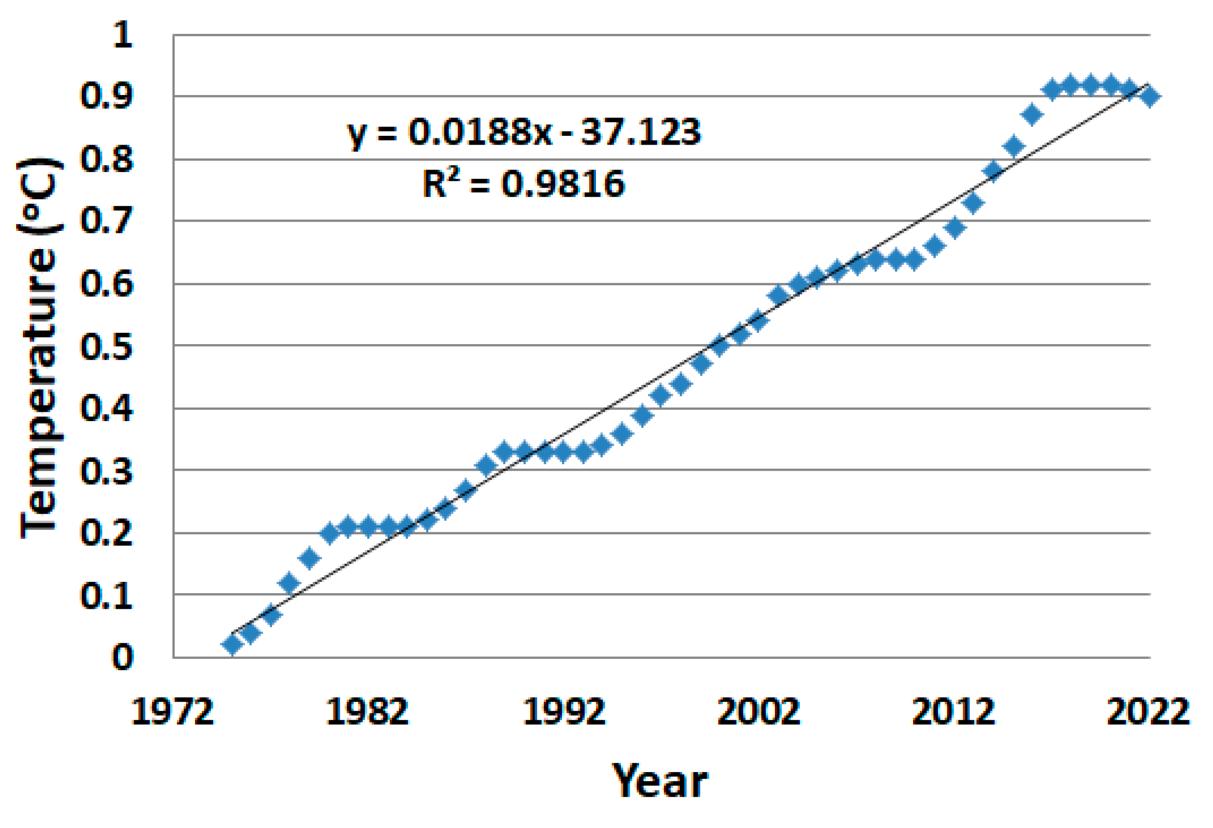
Table 2.
ASG requirements for land and space.
| Earth Brightening | Space | ||||||
| Parameters | Pavements | Desert Treatment | UHIs |
Earth (Sea) Mirrors |
L1 Space Shading Parameters | Stratosphere Injections | |
| DPASG(Wm-2) | -0.01465 | -0.01465 | -0.0147 | -0.01465 | DPASG(Wm-2) | -0.01465 | -0.01465 |
| XC, XS | 0.47, 1 | 0.92, 1 | 0.47, 1 | 0.7, 1 | XC, XS | 1, 4 | 1, 1 |
| 0.3 | 0.44 | 0.1 | 0.75 | 0.7 | 0.3 | ||
| HT | 1 | 1 | 3 | 2 (1) | HT | 1 | 1 |
| 2.15 | 2.15 | 2.15 | 2.15 | 2.15 | 2.15 | ||
| Earth Brightening Results | L1 Space Disc Results | CaCO3 Injec. | |||||
| AT/AE | 0.0305% | 0.0106% | 0.031% | 0.0041% (0.0082%) |
AT/AE Earth Shade | 0.00154% | 0.0144%/eff |
| AT (Mi2) | 60,035 | 20,940 | 60,035 | 8061 (16,124) | Shade AT (Mi2, km2) | 3023, 7843 | ~27,924,~74,322 |
| Radius (Mi) | 138 | 81.6 | 138 | 51 (71.6) | Shade Radius (Mi, km) | 31, 50 | ~94.3, ~153.8 |
| AT (km2) | 1.56E+05 | 5.42E+04 | 1.6E+05 | 2.1E+04 (4.2E+04) | Disc Area (Mi2, km2)* | 3023, 7843 | - |
| Radius (km) | 223 | 131 | 223 | 81.6 (115) | Disc Radius (Mi, km)* | 31, 50 | - |
*Depends on Sun blocking efficiency of the disc and actual distance relative to L1.
Table 3.
ASG potential hotspot possible requirements.
| T2, T1 XC |
61oC, 33oC 0.5, 0.47 |
| AF | 4.3 |
| DPASG(Wm-2) | -0.01465 |
| AT/AE | 0.0092% |
| AT (Mi2) | 18,011 |
| Radius (Mi) | 76 |
| AT (km2) | 0.47E+05 |
| Radius (km) | 122 |
Disclaimer/Publisher’s Note: The statements, opinions and data contained in all publications are solely those of the individual author(s) and contributor(s) and not of MDPI and/or the editor(s). MDPI and/or the editor(s) disclaim responsibility for any injury to people or property resulting from any ideas, methods, instructions or products referred to in the content. |
© 2023 by the authors. Licensee MDPI, Basel, Switzerland. This article is an open access article distributed under the terms and conditions of the Creative Commons Attribution (CC BY) license (http://creativecommons.org/licenses/by/4.0/).
Copyright: This open access article is published under a Creative Commons CC BY 4.0 license, which permit the free download, distribution, and reuse, provided that the author and preprint are cited in any reuse.


