Submitted:
23 July 2023
Posted:
25 July 2023
You are already at the latest version
Abstract
Keywords:
I. Introduction
II. Literature Review
III. Methodology
- AWID3 includes recently identified attacks against the 802.11 protocol, including well-known instances like Krack and kr00k. This inclusion enables researchers to investigate and create practical defenses against these particular dangers within the framework of the dataset.
- A network’s packet-level details are contained in the pcap format used to supply the data in AWID3. Researchers now have access to extensive data that can be utilized to assess network features and meet specific research objectives. The dataset also includes the Pairwise Master Key (PMK) and TLS keys.
- The enterprise versions of the 802.11 standards are the main emphasis of AWID3. Stronger security features, like support for alternative network architectures and the use of Protected Management Frames (PMF), which were introduced with the 802.11w revision, are often present in these versions. By focusing on enterprise versions, the dataset is more applicable to actual security issues.
- The link layer of the 802.11 protocol is initially targeted via attacks on the AWID3 dataset. These assaults, nevertheless, quickly spread to higher layers, affecting protocols that run at different levels of the network stack. Researchers can examine the interrelated nature of network vulnerabilities due to this comprehensive perspective of attack propagation.
- Every scenario in the dataset is covered in great detail by AWID3. Researchers may undertake detailed analysis and evaluation with the help of this documentation, which also helps them grasp the nuances of assault scenarios.
A. Structure of AWID3 Dataset
- -
- Deauthentication Attack.
- -
- Disassociation Attack.
- -
- Re-association Attack.
- -
- Rogue AP Attack.
- -
- Krack Attack.
- -
- Kr00k Attack.
- -
- SSH Brute Force Attack.
- -
- Botnet Attack.
- -
- Malware.
- -
- SSDP Amplification.
- -
- SQL Injection Attack.
- -
- Evil Twin.
- -
- Website spoofing.
- 1)
-
Krack Attack: The Krack attack has been noted as a potential security risk to the current encryption techniques used to preserve and protect Wi-Fi networks for the past 15 years. Publicly available information on the Krack attack includes information about the attack itself. There is no guarantee that every device will have a patch and be protected from these attacks coming from any networked point [37,38]. The four-way handshake procedure, which is a crucial part of the IEEE802.11 protocol, has a serious weakness that allows any attacker to decode a user’s communication without eavesdropping on the handshake or knowing the encryption key, according to In [39] study. This flaw results from the Pairwise Transient Key (PTK) installation process’ use of a particular message counter. It is vital to look at how keystreams are used in the encryption process in order to comprehend the decryption process. The plaintext and keystream are merged using the XOR (exclusive OR) technique to create the encrypted message that is sent from the client to the Access Point (AP). The PTK, which is derived using the AES (Advanced Encryption Standard), is scrambled with a number of other factors to create the keystream. The vulnerability, though, only exists in the XOR operation’s last phase. The logic flow of this step is connected to a fundamental mathematical feature that is exploited by the KRACK vulnerability. Equation (1) shows how the plaintext (P) and keystream (KS), as shown in the paper, are combined to create the ciphertext (E). The KRACK hack uses this defect in the XOR method to decrypt the encrypted communications, putting the security of wireless networks using the IEEE 802.11 standard at risk.
- 2)
- Kr00k Attack: Some WiFi traffic that has been encrypted with WPA2 can be decrypted by a vulnerability called Kr00k. Security company ESET discovered the vulnerability in 2019. According to ESET, this loophole affects more than a billion devices. Devices with Wi-Fi chips that have not yet received a patch from Broadcom or Cypress are vulnerable to Kr00k. The majority of modern Wi-Fi-enabled devices, including smartphones, tablets, laptops, and Internet of Things (IoT) devices, use these Wi-Fi chips [41]. Table 1 highlighted the main difference between Krack and Kr00k attacks.
B. Preprocessing steps
- 1)
-
Decision tree: the process for building a decision tree and the most commonly used criteria for splitting the data [42]:
- -
- Calculate an impurity measure for the entire dataset (e.g., Gini impurity or entropy).
- -
- For each feature, calculate the impurity measure of splitting the data based on the values of that feature.
- -
- Choose the feature that produces the lowest impurity measure after splitting the data.
- -
- Split the data based on the chosen feature and repeat the process for each resulting subset of data until a stopping criterion is met (e.g., a maximum depth is reached or the number of samples in a leaf node is below a certain threshold).
- 2)
- Ensemble classifiers: combine multiple individual classifiers into a single ensemble classifier to improve the overall predictive performance. There are different types of ensemble classifiers, such as bagging, boosting, and stacking, and the equations used for each type can vary.
- 3)
- SVM: Support Vector Machine (SVM) is a popular machine learning algorithm for classification, regression, and outlier detection. The main idea behind SVM is to find a hyperplane that separates the data into different classes with the largest margin possible. The equations used in SVM [43]:


- 4)
- Kernal: A kernel function is a function that maps the input data into a higher-dimensional space, where it is easier to find a separating hyperplane. The equation of linear Kernal [44]:

- 5)
- KNN: K-Nearest Neighbors (KNN) is a simple yet effective machine learning algorithm used for classification and regression tasks. The basic idea behind KNN is to find the K nearest training samples to a given test sample based on a distance metric, and then use the labels of the K nearest neighbors to predict the label of the test sample. The equation of KNN can be represented as follow [42]:

- 6)
-
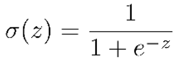
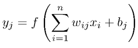
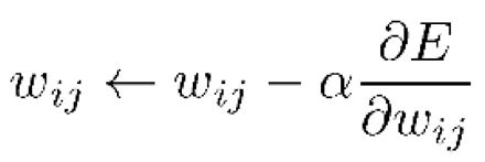
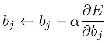
Neural Network: Neural Networks are a powerful class of machine learning algorithms that are inspired by the structure and function of the human brain. A neural network consists of multiple layers of interconnected processing units called neurons, and the input data is processed through the network in a forward pass, with the output of each layer serving as the input to the next layer. Some equations used in neural networks [45]:
- -
- Activation function://
- -
- Forward pass:
- -
- Backpropagation:
 and
and  are the partial derivatives of the error
concerning the weights and biases, respectively.
are the partial derivatives of the error
concerning the weights and biases, respectively.- 1)
-
Detecting Krack attack: According to the importance of preprocessing step as we mentioned before, the preprocessing procedure for the Krack dataset sample was as follows:
- 1-
- Deleting the constant and empty features.
- 2-
- Ignoring features that have more than 60% missing values.
- 3-
- Replace missing values with NaN.

- 2)
-
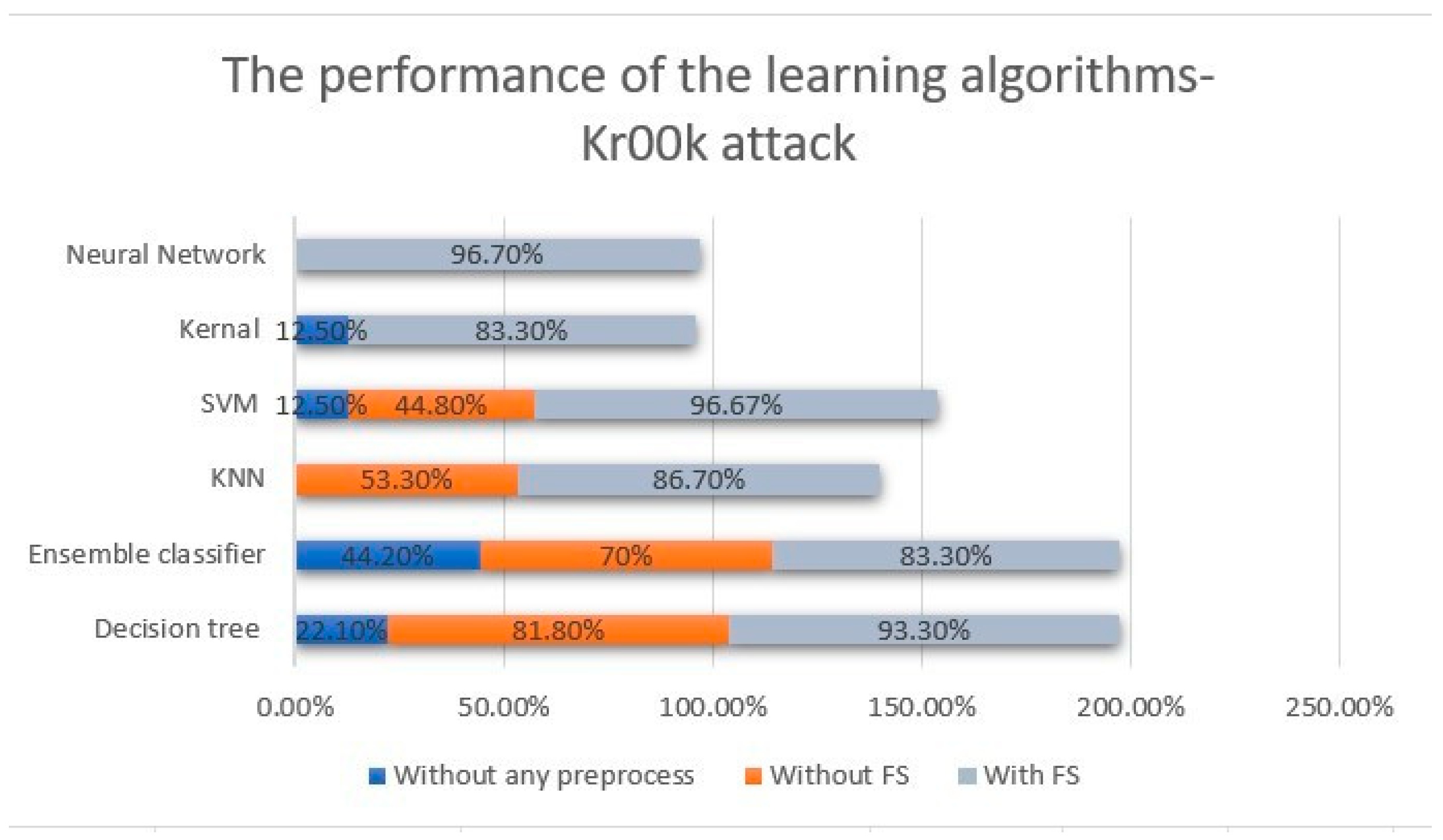
Detecting Kr00k attack: This sample consists of 235,064 instances; (106971 kr00k traffic and 128093 normal ones), the preprocessing procedure for the Krack dataset sample was as follows:
- 1-
- Deleting the constant and empty features.
- 2-
- Ignoring features with more than 60% missing values, the remaining features are 63.
- 3-
- Replace missing values with NaN.
IV. Results and Discussion
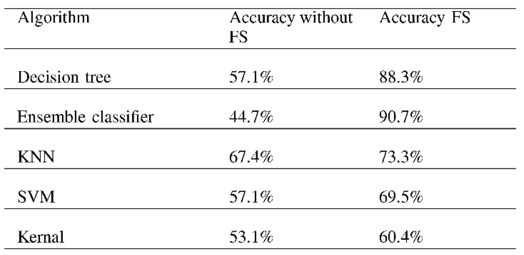 |
- -
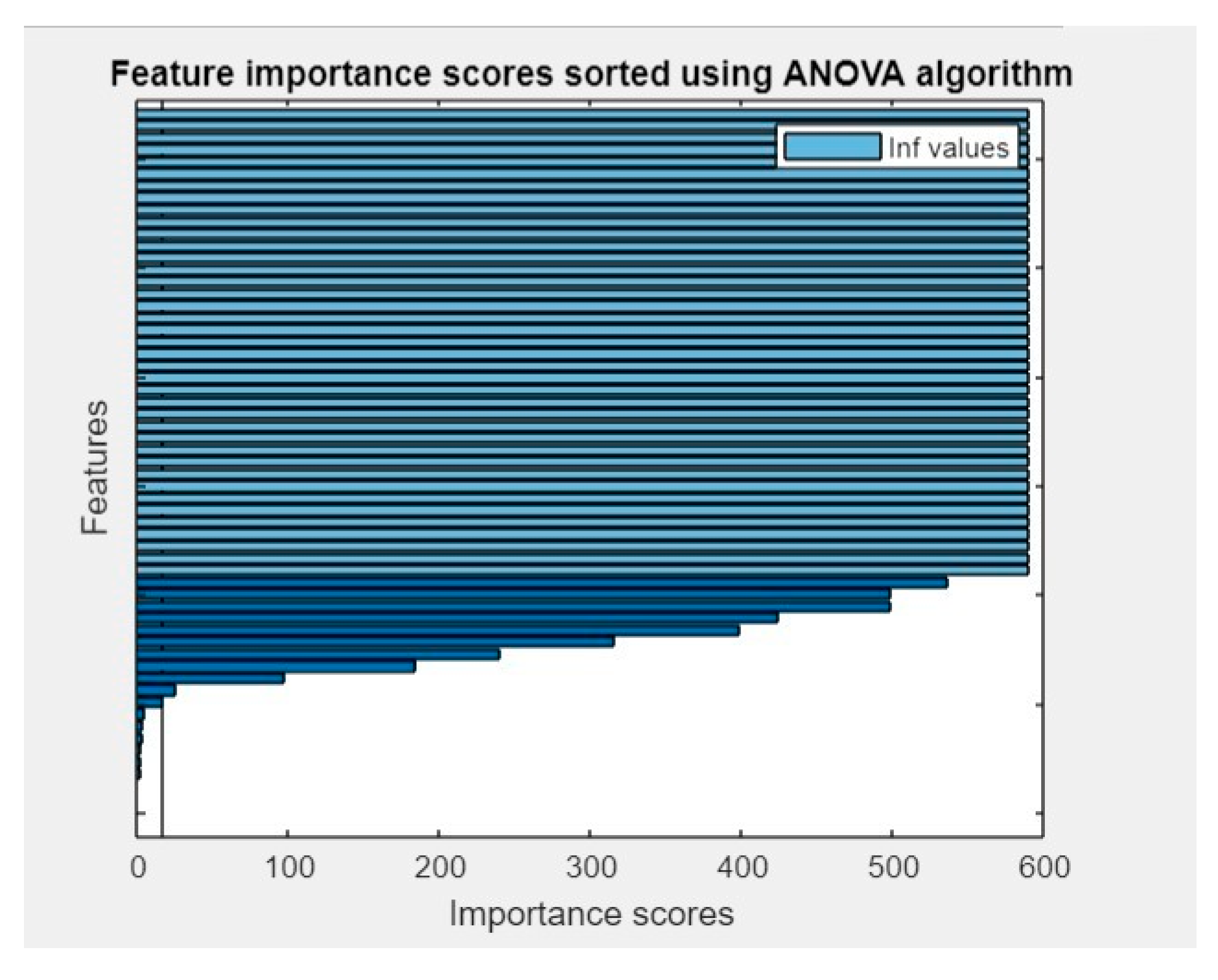
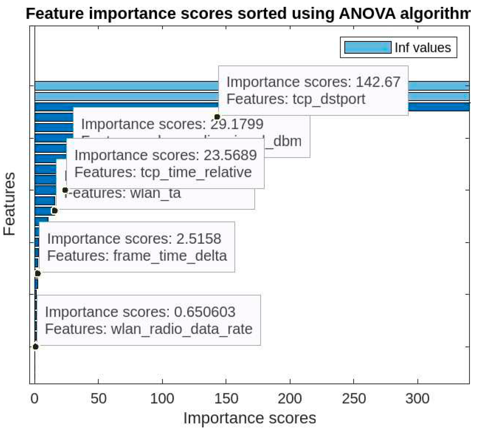
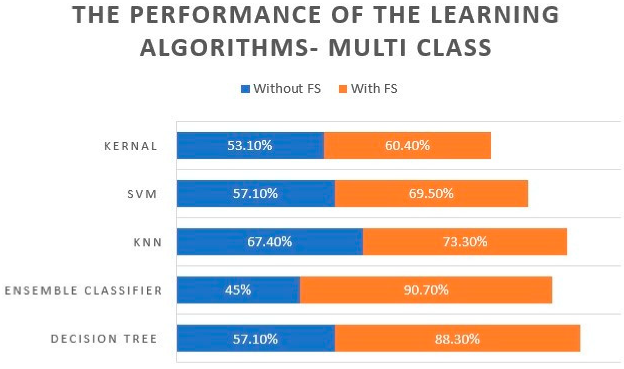
- High dimensionality refers to a high number of features in the dataset. So it’s important to transform the data from a high- dimensional space into a low-dimensional space so that the low-dimensional representation retains some meaningful properties of the original data, ideally close to its intrinsic dimension [50]. we solved this problem using the ANOVA FS techniques, where the performance of the algorithms shows clear improvement in accuracy results when we reduce the high dimensionality for the dataset.
- -
- Overfitting of the dataset: it occurs when a statistical model fits exactly against its training data [51]. Actually, when performing the ML model to the data without solving the overfitting problem, the accuracy results will be almost 100% or 99.99% which is not reliable performance. We solved this problem in the pre-processing step by getting rid of the features that coping the label, in addition to the importance of FS in solving this problem.
- -
- imbalanced data: Unbalanced refers to a classification data set with skewed class proportions. We solved this problem by taking almost the same number of instances for attack and benign in the three experiments.
Comparing our findings with previous studies
V. Conclusion
References
- Alraih, S.; Shayea, I.; Behjati, M.; Nordin, R.; Abdullah, N.F.; Abu-Samah, A.; Nandi, D. Revolution or Evolution? Technical Requirements and Considerations towards 6G Mobile Communications. Sensors 2022, 22, 762. [Google Scholar] [CrossRef]
- Chettri, L.; Bera, R. A Comprehensive Survey on Internet of Things (IoT) Toward 5G Wireless Systems. IEEE Internet Things J. 2019, 7, 16–32. [Google Scholar] [CrossRef]
- Ahn, V.T.H.; Ma, M. A Secure Authentication Protocol with Performance Enhancements for 4G LTE/LTE-A Wireless Networks. In Proceedings of the 2021 3rd International Electronics Communication Conference (IECC), Ho Chi Minh City, Vietnam, 8–10 July 2021; pp. 28–36. [Google Scholar]
- Prabha, P.A.; Arjun, N.; Gogul, J.; Prasanth, S.D. Two-Way Economical Smart Device Control and Power Consumption Prediction System. In Proceedings of the International Conference on Recent Trends in Computing, Ghaziabad, India, 4–5 June 2021; Springer: Singapore, 2022; pp. 415–429. [Google Scholar]
- Liyanage, M.; Braeken, A.; Jurcut, A.D.; Ylianttila, M.; Gurtov, A. Secure communication channel architecture for Software Defined Mobile Networks. Comput. Netw. 2017, 114, 32–50. [Google Scholar] [CrossRef]
- Gurtov, A.; Liyanage, M.; Ylianttila, M. Software Defined Mobile Networks (SDMN): Beyond LTE Network Architecture; John Wiley & Sons: Hoboken, NJ, USA, 2015. [Google Scholar]
- Park, J.H.; Rathore, S.; Singh, S.K.; Salim, M.M.; Azzaoui, A.; Kim, T.W.; Pan, Y.; Park, J.H. A comprehensive survey on core technologies and services for 5g security: Taxonomies, issues, and solutions. Hum.-Centric Comput. Inf. Sci. 2021, 11, 3. [Google Scholar]
- Gupta, S.; Parne, B.L.; Chaudhari, N.S. Security vulnerabilities in handover authentication mechanism of 5g network. In Proceedings of the 2018 First International Conference on Secure Cyber Computing and Communication (ICSCCC), Jalandhar, India, 15–17 December 2018; IEEE: Piscataway, NJ, USA, 2018; pp. 369–374. [Google Scholar]
- Borgaonkar, R.; Tøndel, I.A.; Degefa, M.Z.; Jaatun, M.G. Improving smart grid security through 5G enabled IoT and edge computing. Concurr. Comput. Pract. Exp. 2021, 33, e6466. [Google Scholar] [CrossRef]
- Gonzalez, A.J.; Grønsund, P.; Dimitriadis, A.; Reshytnik, D. Information security in a 5g facility: An implementation experience. In Proceedings of the 2021 Joint European Conference on Networks and Communications & 6G Summit (EuCNC/6G Summit), Porto, Portugal, 8–11 June 2021; IEEE: Piscataway, NJ, USA, 2021; pp. 425–430. [Google Scholar]
- Kim, H. 5G core network security issues and attack classification from network protocol perspective. J. Internet Serv. Inf. Secur. 2020, 10, 1–15. [Google Scholar]
- Mohan, J.P.; Sugunaraj, N.; Ranganathan, P. Cyber security threats for 5g networks. In Proceedings of the 2022 IEEE International Conference on Electro Information Technology (eIT), Mankato, MN, USA, 19–22 May 2022; IEEE: Piscataway, NJ, USA, 2022; pp. 446–454. [Google Scholar]
- Tsiknas, K.; Taketzis, D.; Demertzis, K.; Skianis, C. Cyber Threats to Industrial IoT: A Survey on Attacks and Countermeasures. IoT 2021, 2, 163–186. [Google Scholar] [CrossRef]
- Muthuramalingam, S.; Thangavel, M.; Sridhar, S. A review on digital sphere threats and vulnerabilities. In Combating Security Breaches and Criminal Activity in the Digital Sphere; IGI Global: Hershey, PA, USA, 2016; pp. 1–21. [Google Scholar]
- Klaine, P.V.; Imran, M.A.; Onireti, O.; Souza, R.D. A Survey of Machine Learning Techniques Applied to Self-Organizing Cellular Networks. IEEE Commun. Surv. Tutor. 2017, 19, 2392–2431. [Google Scholar] [CrossRef]
- Klautau, A.; Batista, P.; Gonza, N.; Wang, Y.; Heath, R.W. 5G mimo data for machine learning: Application to beam-selection using deep learning. In Proceedings of the 2018 Information Theory and Applications Workshop (ITA), San Diego, CA, USA, 11–16 February 2018; IEEE: Piscataway, NJ, USA, 2018; pp. 1–9. [Google Scholar]
- Kafle, V.P.; Fukushima, Y.; Martinez-Julia, P.; Miyazawa, T. Consideration on Automation of 5G Network Slicing with Machine Learning. In Proceedings of the 2018 ITU Kaleidoscope: Machine Learning for a 5G Future, Santa Fe, Argentina, 26–28 November 2018. [Google Scholar]
- Sofi, I.B.; Gupta, A. A survey on energy efficient 5G green network with a planned multi-tier architecture. J. Netw. Comput. Appl. 2018, 118, 1–28. [Google Scholar] [CrossRef]
- Ioannou, I.; Christophorou, C.; Vassiliou, V.; Pitsillides, A. A distributed AI/ML framework for D2D Transmission Mode Selection in 5G and beyond. Comput. Netw. 2022, 210, 108964. [Google Scholar] [CrossRef]
- Nassef, O.; Sun, W.; Purmehdi, H.; Tatipamula, M.; Mahmoodi, T. A survey: Distributed Machine Learning for 5G and beyond. Comput. Netw. 2022, 207, 108820. [Google Scholar] [CrossRef]
- Babu, K.V.; Das, S.; Sree, G.N.J.; Patel, S.K.; Saradhi, M.P.; Tagore, M. Design and development of miniaturized MIMO antenna using parasitic elements and Machine learning (Ml) technique for lower sub 6 GHz 5G applications. AEU-Int. J. Electron. Commun. 2022, 153, 154281. [Google Scholar] [CrossRef]
- Yang, L.; Li, J.; Yin, L.; Sun, Z.; Zhao, Y.; Li, Z. Real-Time Intrusion Detection in Wireless Network: A Deep Learning-Based Intelligent Mechanism. IEEE Access 2020, 8, 170128–170139. [Google Scholar] [CrossRef]
- Berisha, V.; Krantsevich, C.; Hahn, P.R.; Hahn, S.; Dasarathy, G.; Turaga, P.; Liss, J. Digital medicine and the curse of dimensionality. NPJ Digit. Med. 2021, 4, 153. [Google Scholar] [CrossRef]
- Lee, S.J.; Yoo, P.D.; Asyhari, A.T.; Jhi, Y.; Chermak, L.; Yeun, C.Y.; Taha, K. IMPACT: Impersonation attack detection via edge computing using deep autoencoder and feature abstraction. IEEE Access 2020, 8, 65520–65529. [Google Scholar] [CrossRef]
- Kolias, C.; Kambourakis, G.; Stavrou, A.; Gritzalis, S. Intrusion Detection in 802.11 Networks: Empirical Evaluation of Threats and a Public Dataset. IEEE Commun. Surv. Tutor. 2015, 18, 184–208. [Google Scholar] [CrossRef]
- Chatzoglou, E.; Kambourakis, G.; Kolias, C. Empirical evaluation of attacks against IEEE 802.11 enterprise networks: The awid3 dataset. IEEE Access 2021, 9, 34188–34205. [Google Scholar] [CrossRef]
- Kolias, C.; Kolias, V.; Kambourakis, G. TermID: A distributed swarm intelligence-based approach for wireless intrusion detection. Int. J. Inf. Secur. 2017, 16, 401–416. [Google Scholar] [CrossRef]
- Aminanto, M.E.; Choi, R.; Tanuwidjaja, H.C.; Yoo, P.D.; Kim, K. Deep Abstraction and Weighted Feature Selection for Wi-Fi Impersonation Detection. IEEE Trans. Inf. Forensics Secur. 2017, 13, 621–636. [Google Scholar] [CrossRef]
- Diro, A.; Chilamkurti, N. Leveraging LSTM Networks for Attack Detection in Fog-to-Things Communications. IEEE Commun. Mag. 2018, 56, 124–130. [Google Scholar] [CrossRef]
- Sethuraman, S.C.; Dhamodaran, S.; Vijayakumar, V. Intrusion detection system for detecting wireless attacks in IEEE 802.11 networks. IET Netw. 2019, 8, 219–232. [Google Scholar] [CrossRef]
- Kasongo, S.M.; Sun, Y. A deep learning method with wrapper based feature extraction for wireless intrusion detection system. Comput. Secur. 2020, 92, 101752. [Google Scholar] [CrossRef]
- Zhou, Y.; Cheng, G.; Jiang, S.; Dai, M. Building an efficient intrusion detection system based on feature selection and ensemble classifier. Comput. Netw. 2020, 174, 107247. [Google Scholar] [CrossRef]
- Hacılar, H.; Aydın, Z.; Güngör, V.Ç. Intrusion Detection with Bayesian Optimization on Imbalance Wired Wireless and Software-Defined Networking Traffics. Available online: https://www.researchgate.net/publication/357833330_Intrusion_Detection_with_Bayesian_Optimization_on_Imbalance_Wired_Wireless_and_Software-Defined_Networking_Traffics (accessed on 1 July 2023).
- Wilson, R.; Linekar, R. Towards effective wireless intrusion detection using awid dataset. 2021. [Google Scholar]
- Bhandari, S.; Kukreja, A.K.; Lazar, A.; Sim, A.; Wu, K. Feature selection improves tree-based classification for wireless intrusion detection. In Proceedings of the 3rd International Workshop on Systems and Network Telemetry and Analytics, Stockholm, Sweden, 23 June 2020; pp. 19–26. [Google Scholar]
- Rahman, M.A.; Asyhari, A.T.; Leong, L.; Satrya, G.; Tao, M.H.; Zolkipli, M. Scalable machine learning-based intrusion detection system for iot-enabled smart cities. Sustain. Cities Soc. 2020, 61, 102324. [Google Scholar] [CrossRef]
- Agrawal, A.; Chatterjee, U.; Maiti, R.R. Ktracker: Passively tracking krack using ml model. In Proceedings of the Twelveth ACM Conference on Data and Application Security and Privacy, Baltimore, MD, USA, 24–27 April 2022; pp. 364–366. [Google Scholar]
- Fontes, R.D.R.; Rothenberg, C.E. On the Krack Attack: Reproducing Vulnerability and a Software-Defined Mitigation Approach, (2018). Available online: https://api.semanticscholar.org/CorpusID:51995777 (accessed on 1 July 2023).
- Vanhoef, M.; Piessens, F. Key reinstallation attacks: Forcing nonce reuse in wpa2. In Proceedings of the 2017 ACM SIGSAC Conference on Computer and Communications Security, Dallas, TX, USA, 30 October–3 November 2017; pp. 1313–1328. [Google Scholar]
- Kohlios, C.P.; Hayajneh, T. A Comprehensive Attack Flow Model and Security Analysis for Wi-Fi and WPA3. Electronics 2018, 7, 284. [Google Scholar] [CrossRef]
- Čermák, M.; Svorenčík, S.; Lipovský, R. Kr00k-cve-2019-15126–Serious Vulnerability Deep Inside Your Wi-Fi Encryption; ESET Research White Paper, Bratislava, Slovak Republic; 2020. Available online: https://web-assets.esetstatic.com/wls/2020/02/ESET_Kr00k.pdf (accessed on 1 July 2023).
- Hastie, T.; Tibshirani, R.; Friedman, J.H.; Friedman, J.H. The Elements of Statistical Learning: Data Mining, Inference, and Prediction; Springer: Berlin/Heidelberg, Germany, 2009; Volume 2. [Google Scholar]
- Cortesc, V. Support vector networks. Mach. Learn. 1995, 20, 273–297. [Google Scholar] [CrossRef]
- Shawe-Taylor, J.; Cristianini, N. Kernel Methods for Pattern Analysis; Cambridge University Press: Cambridge, UK, 2004. [Google Scholar]
- Goodfellow, I.; Bengio, Y.; Courville, A. Deep Learning; MIT Press: Cambridge, MA, USA, 2016. [Google Scholar]
- Alam, S.; Yao, N. The impact of preprocessing steps on the accuracy of machine learning algorithms in sentiment analysis. Comput. Math. Organ. Theory 2019, 25, 319–335. [Google Scholar] [CrossRef]
- Go, A.; Bhayani, R.; Huang, L. Twitter Sentiment Classification Using Distant Supervision; CS224N Project Report; Stanford University: Stanford, CA, USA, 2009. [Google Scholar]
- Kubik, C.; Knauer, S.M.; Groche, P. Smart sheet metal forming: Importance of data acquisition, preprocessing and transformation on the performance of a multiclass support vector machine for predicting wear states during blanking. J. Intell. Manuf. 2022, 33, 259–282. [Google Scholar] [CrossRef]
- Nasiri, H.; Alavi, S.A. A Novel Framework Based on Deep Learning and ANOVA Feature Selection Method for Diagnosis of COVID-19 Cases from Chest X-Ray Images. Comput. Intell. Neurosci. 2022, 2022, 4694567. [Google Scholar] [CrossRef]
- Zebari, R.; Abdulazeez, A.; Zeebaree, D.; Zebari, D.; Saeed, J. A Comprehensive Review of Dimensionality Reduction Techniques for Feature Selection and Feature Extraction. J. Appl. Sci. Technol. Trends 2020, 1, 56–70. [Google Scholar] [CrossRef]
- Belkin, M.; Hsu, D.; Ma, S.; Mandal, S. Reconciling modern machine-learning practice and the classical bias–variance trade-off. Proc. Natl. Acad. Sci. USA 2019, 116, 15849–15854. [Google Scholar] [CrossRef] [PubMed]
- Alperin, K.; Joback, E.; Shing, L.; Elkin, G. A framework for unsupervised classificiation and data mining of tweets about cyber vulnerabilities. arXiv 2021, arXiv:2104.11695. [Google Scholar]
- Chatzoglou, E.; Kambourakis, G.; Smiliotopoulos, C.; Kolias, C. Best of both worlds: Detecting application layer attacks through 802.11 and non-802.11 features. Sensors 2022, 22, 5633. [Google Scholar] [CrossRef] [PubMed]
- Muhati, E.; Rawat, D.B. Asynchronous Advantage Actor-Critic (A3C) Learning for Cognitive Network Security. In Proceedings of the 2021 Third IEEE International Conference on Trust, Privacy and Security in Intelligent Systems and Applications (TPS-ISA), Virtual, 13–15 December 2021; pp. 106–113. [Google Scholar]
- Zheng, C.; Zang, M.; Hong, X.; Bensoussane, R.; Vargaftik, S.; Ben-Itzhak, Y.; Zilberman, N. Automating in-network machine learning. arXiv 2022, arXiv:2205.08824. [Google Scholar]

 |
| Samples | Attack | Normal |
| First Sample | 106971 kr00k traffic | 128093 |
| Second Sample | 33180 Krack traffic | 34000 |
| Algorithm | Accuracy / kr00k attack |
Accuracy / Krack attack |
| Decision tree | 22.10% | 50% |
| Ensemble classifier | 44.20% | 50% |
| SVM | 12.50% | failed |
| Kernal | 12.50% | failed |
| Algorithm | Accuracy | True Positive Rate |
False Nega- tive Rate |
| Decision tree | 95.1% | 90% | 10% |
| Ensemble classi- | 50.6% | 50.6% | 49.4% |
| fier | |||
|
KNN |
73.8% |
48.3% |
51.7% |
| SVM | 50.6% | 50.6% | 49.4% |
| Algorithm | Accuracy | True Positive Rate | False Negative Rate | AUC |
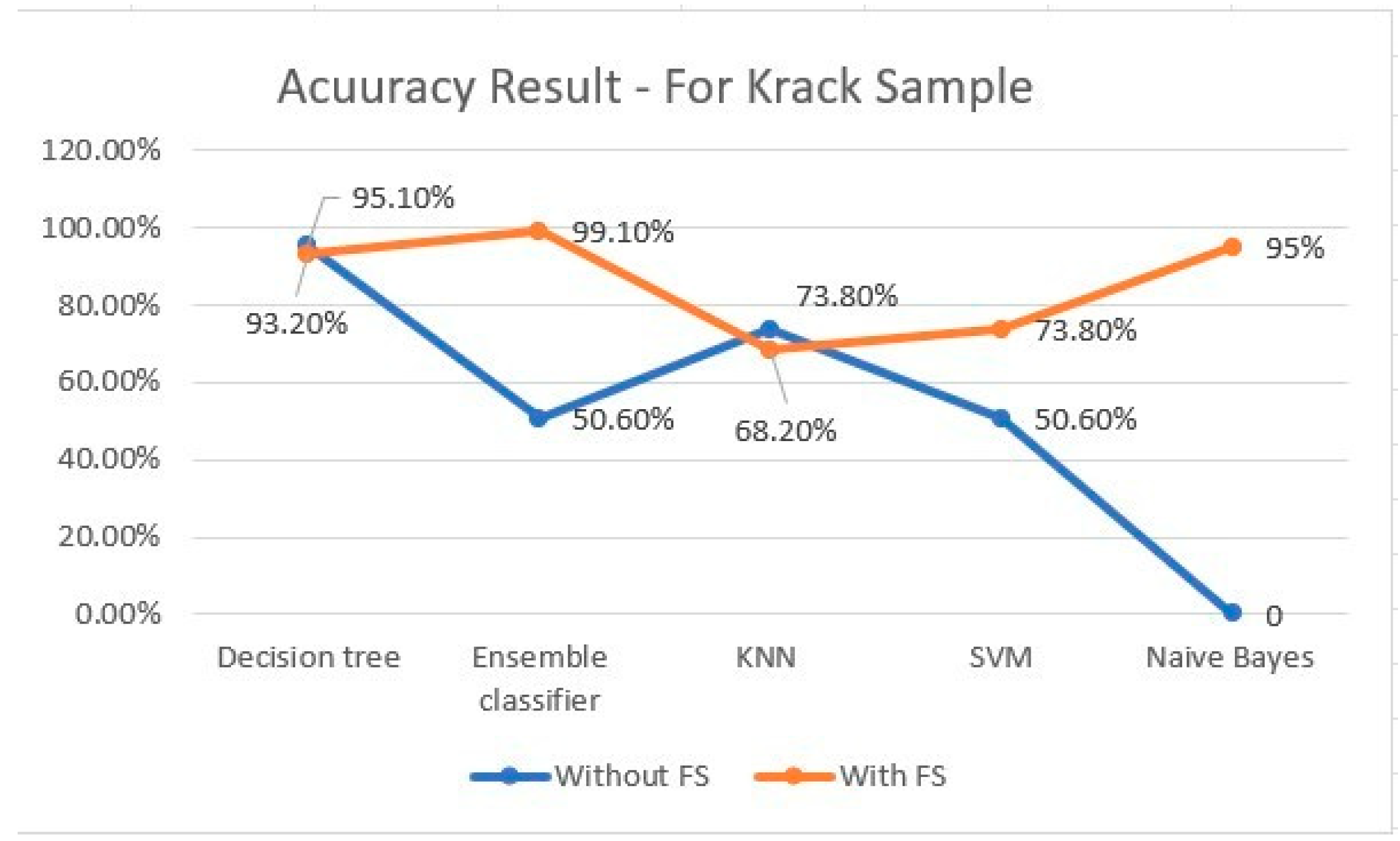
| Decision tree | 93.2% | 86.6% | 13.4% | 0.964 |
| Naive Bayes | 95% | 97.7% | 2.3% | 0.9891 |
| Ensemble classi- | 99.1% | 98.2% | 1.8% | 0.9998 |
| fier | ||||
|
KNN |
68.2% |
35.8% |
64.2% |
0.9995 |
| SVM | 73.8% | 46.9% | 53.1% | 1 |
| Algorithm | Accuracy | True Positive Rate |
False Nega- tive Rate |
| Decision tree | 81.8% | 60% | 40% |
| Ensemble classi- | 70% | 45.3% | 54.7% |
| fier | |||
|
KNN |
53.3% |
53.3% |
46.7% |
| SVM | 44.8% | 40.7% | 59.3% |
| Algorithm | Accuracy |
| Decision tree | 93.3% |
| Ensemble classifier | 83.3% |
| KNN | 86.7% |
| SVM | 96.67% |
| Neural Network | 96.7% |
| Kernal | 83.3% |
| Refrence | Year | Description | Accuracy |
| [37] | 2022 | They monitored numerous wireless channels to detect Krack attack | 93.0% |
| [52] | 2021 | Proposed a framework for Cyber Vulnerabilities, including Kr00k | 88.52% |
| [53] | 2022 | Proposed a model to detect the application layer attacks | 96.7% |
| [54] | 2021 | proposed an automated network scanning and data-mining technique for Network IDS | 98.68% |
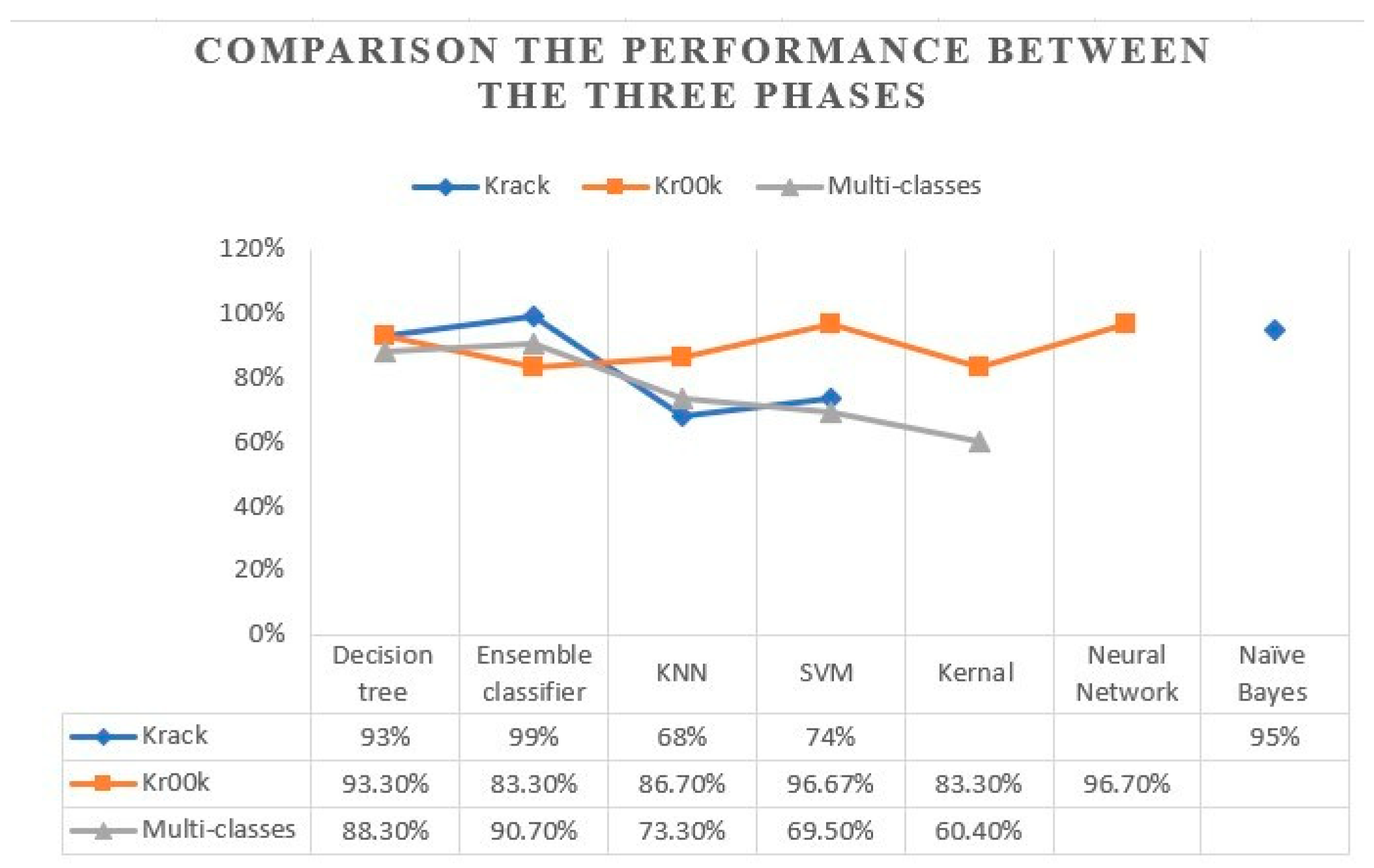
| Our work | We focused on the IEEE 802.11 vulnerabilities, by proposing a model to detect Krack and kr00k attacks using ML tech- niques. | Phase 1: 99% Phase 2: 96.7% phase 3: 90.7% |
Disclaimer/Publisher’s Note: The statements, opinions and data contained in all publications are solely those of the individual author(s) and contributor(s) and not of MDPI and/or the editor(s). MDPI and/or the editor(s) disclaim responsibility for any injury to people or property resulting from any ideas, methods, instructions or products referred to in the content. |
© 2023 by the authors. Licensee MDPI, Basel, Switzerland. This article is an open access article distributed under the terms and conditions of the Creative Commons Attribution (CC BY) license (https://creativecommons.org/licenses/by/4.0/).


