Scaled-Invariant Extended Quasi-Lindley Model: Properties, Estimation and Application

Preprint

Article

Scaled-Invariant Extended Quasi-Lindley Model: Properties, Estimation and Application

Altmetrics

Downloads

115

Views

Comments

A peer-reviewed article of this preprint also exists.

Mohamed Kayid,Abdulrahman Abouammoh,

Ghadah Alomani^*

Mohamed Kayid,Abdulrahman Abouammoh,

Ghadah Alomani^*

This version is not peer-reviewed

Submitted:

22 July 2023

Posted:

25 July 2023

You are already at the latest version

Alerts

Abstract

In many research fields, statistical probability models are often used to analyze real-world data. However, data from many fields, such as the environment, economics, and health care, do not necessarily fit traditional models. New empirical models need to be developed to improve their fit. In this paper, we explore a further extension of the quasi-Lindley model. Maximum likelihood, least square error, Anderson-Darling algorithm, and expectation-maximization algorithm are four techniques for estimating the parameters under study. All techniques provide accurate and reliable estimates of the parameters. However, the mean square error of the expectation maximization approach was lower. The usefulness of the proposed model was demonstrated by analyzing a dynamical systems data set, and the analysis shows that it outperforms the other models in all statistical models considered.

Keywords:

Subject: Computer Science and Mathematics - Probability and Statistics

1. Introduction

A Lindley model that is simple and remarkably flexible in application was proposed by [1]. It is characterized by the probability density function (pdf)

f (x) = \frac{ξ^{2}}{ξ + 1} (1 + x) e^{- ξ x}, ξ > 0, x \geq 0,

(1)

which is a mixture of two gamma models

G (1, ξ)

and

G (2, ξ)

with weights,

ξ / ξ + 1

and

1 / ξ + 1,

respectively. Numerous studies have been conducted on the Lindley model. For example, many properties, extensions, and applications of the model have been studied in [2,3,4,5,6,7,8,9,10,11,12,13,14,15,16,17,18,19,20,21]. A scale-invariant version of the Lindley model, namely the quasi Lindley (QL), with the pdf

f (x) = \frac{ξ}{α + 1} (α + ξ x) e^{- ξ x}, α > 0, ξ > 0, x \geq 0,

(2)

which is a mixture of two gamma models

G (1, ξ)

and

G (2, ξ)

with weights

α / α + 1

and

1 / α + 1

respectively proposed by [22].

A family of models characterized by

f (x)

is said to be scale-invariant if the transformation from

x

k x

lies within the family

k

pdf times a Jacobi associated with that transformation. Thus, if you change the scale of measurement or the unit of

x

, the fit remains invariant. For instance, a lifetime can be measured in days, hours, or minutes, and the unit of measurement does not affect inferences about lifetimes. Since scale invariance is an essential property of lifetime models, this model has attracted considerable interest. A comparison of the maximum likelihood estimator (MLE) and the expectation-maximization (EM) algorithm for estimating the parameters of the QL model studied by [23] and a new scale-invariant extension of the Lindley model proposed by [24].

Many data sets are composed of multiple populations or sources, and the subpopulation associated with each data is usually unknown or recorded. For example, the lifetime of a device or system may be available, but the manufacturer or an event associated with a living being without its geographic location may not be. Such data sets are mixtures because information about some covariates, such as the manufacturer or geographic location, that significantly affect the observations is unknown. For detailed information on mixture models, see [26,27]. The Lindley model and its extensions are examples of mixture models of the gamma distribution that can be useful for describing many real-world applications.

This study proposes a new extension of the scaled invariant QL model, a mixture of three gamma models, and is investigated. Some statistical and reliability properties, such as failure rate (FR), mean residual life (MRL), and p-quantile residual life (p-QRL) functions, are discussed. Four methods for estimating the model parameters are then discussed. It is examined that all methods provide consistent and efficient estimates of the parameters. However, the algorithm for maximizing expected values yields a lower mean square error.

The rest of the article is organized as follows. The scaled-invariant extended quasi-Lindley (EQL) model is explained in Section 2 along with some of its basic properties. Section 3 estimates the parameters of the model using the maximum likelihood (ML) method, the least squares error (LSE) method, the weighted LSE method, and the algorithm EM. A simulation study is then conducted in Section 4 to investigate and compare the behavior of the estimators. The proposed model is fitted to a dataset of intervals between successive air conditioning failures in a Boeing 720 aircraft to show how useful it could be in practice.

2. Scaled-invariant extended QL model

A random variable

X

follows from

E Q L (α, ξ)

if its PDF equals

f (x) = \frac{ξ}{1 + α + α^{2}} (1 + α ξ x + \frac{1}{2} α^{2} ξ^{2} x^{2}) e^{- ξ x}, α \geq 0, ξ > 0, x \geq 0 .

(3)

It shows a mixture of

G (1, ξ)

G (2, ξ)

and

G (3, ξ)

with weights

1 / 1 + α + α^{2}

α / (1 + α + α^{2})

and

α^{2} / (1 + α + α^{2})

respectively. When

α = 0

, it reduces to the exponential model. The reliability function is an important yet very simple measure in reliability theory and survival analysis. For the EQL model it is

R (x) = \frac{1}{(1 + α + α^{2})} (1 + α + α^{2} + α ξ x + α^{2} ξ x + \frac{1}{2} α^{2} ξ^{2} x^{2}) e^{- ξ x} .

(4)

The distribution function is simply related to the reliability function by

F (x) = 1 - R (x)

and the quantile function which is in fact the inverse of the distribution function equals

q (p) = F^{- 1} (p) = \min \{x : F (x) = p\}, 0 < p < 1 .

The quantile function could be used for simulation random samples, estimating the parameters, and computing skewness of the model.

In addition, for the EQL the k-th moment is finite and equal to

E (X^{k}) = \frac{1}{1 + α + α^{2}} \frac{1}{ξ^{k}} [Γ (k + 1) + α Γ (k + 2) + \frac{α^{2}}{2} Γ (k + 3)] .

(5)

2.1. Statistics and Reliability Properties

The FR function at a time

x

expresses the instantaneous risk of fail at

x

given survival up to

x

. For EQL model we have

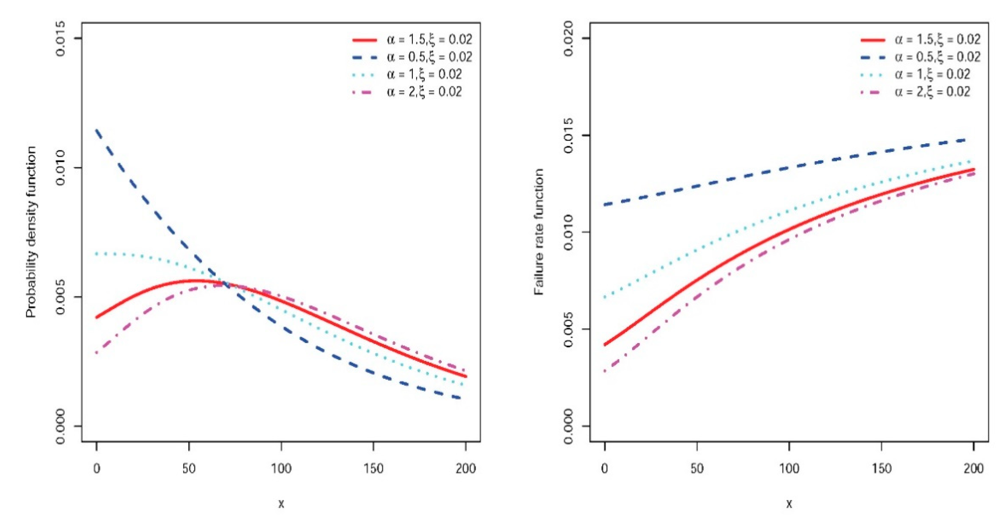
λ (x) = \frac{1 + α ξ x + \frac{1}{2} α^{2} ξ^{2} x^{2}}{1 + α + α^{2} + α ξ x + α^{2} ξ x + \frac{1}{2} α^{2} ξ^{2} x^{2}} ξ .

(6)

Using simple algebra, we can see that the FR function increases from

λ (0) = ξ / 1 + α + α^{2}

{l i m}_{x \to \infty} λ (x) = ξ

Figure 1 shows the shape of the pdf and the FR function for some parameter values. Two other useful and well-known measures in the reliability theory and survival analysis are MRL and

p

-QRL functions. At time

x

, they describe the mean and

p

-quantile of the remaining life for survival to

x

. For EQL, the MRL is obtained by

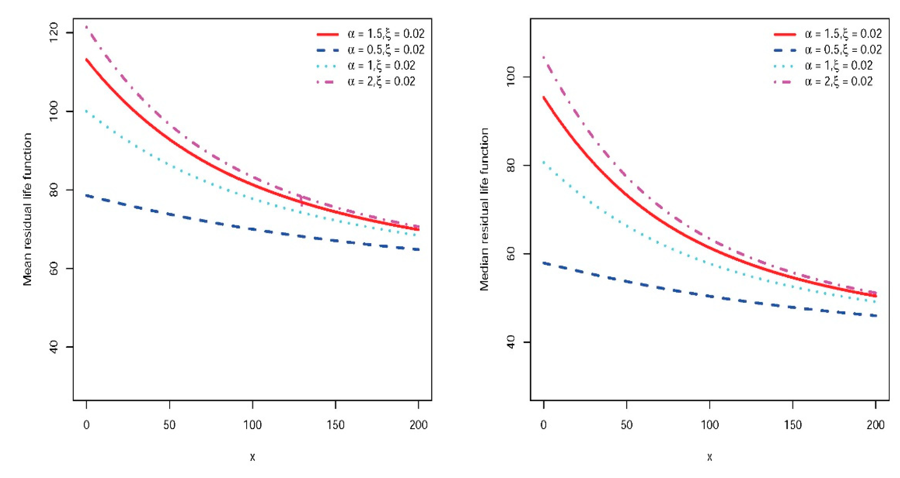
m (x) = \frac{1 + 2 α + 3 α^{2} + (α ξ + 2 α^{2} ξ) x + \frac{1}{2} α^{2} ξ^{2} x^{2}}{1 + α + α^{2} + (α ξ + α^{2} ξ) x + \frac{1}{2} α^{2} ξ^{2} x^{2}} \frac{1}{ξ} .

(7)

Since the FR function is increasing, it follows that the MRL function decreases from

m (0) = \frac{1 + 2 α + 3 α^{2}}{1 + α + α^{2}} \frac{1}{ξ}

\frac{1}{ξ}

at infinity.

The

p

-QRL reads

q_{p} (x) = R^{- 1} ((1 - p) R (x)) - x,

(8)

which can be calculated numerically. Like the MRL, this measure is a decreasing function of

x

. When

p = 0.5

, it is called the median residual life, which is a good alternative to the MRL. In Figure 2, the MRL and the median residual lifetime are plotted for some parameter values and show their similar behavior.

An important concept in reliability theory and survival analysis is orderings between lifetimes. For two lifetimes

X_{1}

and

X_{2}

following reliability functions

R_{1}

and

R_{2}

respectively, we say that,

X_{2}

is greater than

X_{1}

X_{2} \geq X_{1}

, in stochastic if

R_{2} (x) \geq R_{1} (x)

for every

x

. Equivalently we may write

R_{2} \geq R_{1}

in stochastic. There are other useful orderings, e.g., by means of the FR function,

X_{2} \geq X_{1}

, in FR if

h_{1} (x) \geq h_{2} (x)

for every

x

. Moreover,

X_{2} \geq X_{1}

, in MRL and

p

-QRL if

m_{2} (x) \geq m_{1} (x)

and

q_{p, 2} (x) \geq q_{p, 1} (x)

respectively for every

x

. The following result shows that EQL is internally ordered in terms of

α

Proposition 1.

Let

X_{i}

i = 1,2

follows from

E Q L (α, ξ)

and

α_{2} \geq α_{1}

, then

X_{2} \geq X_{1}

in stochastic, FR, MRL and

p

-QRL.

Proof.

To show the FR ordering, the derivative of the FR function in terms of

α

is proportional to

\frac{d λ}{d α} \propto - ({\frac{1}{2} α^{2} ξ^{2} x^{2} + α}^{2} ξ x + 2 α ξ x + 2 α + 1) < 0 .

So, the FR ordering follows. The stochastic, MRL and

p

-QRL orderings follows from FR ordering. See Lai and Xie [28] for relationship between orderings.

◻

3. Estimation

This section discusses some methods for estimating the parameters of the EQL model. In particular, the parameters are estimated using ML, LSE, weighted LSE methods, and an advanced EM algorithm.

3.1. ML method

Let

x_{1}, x_{2}, . . ., x_{n}

represent independent and identically distributed (iid) instances from

E Q L (α, ξ)

. Then, the log-likelihood function is

l (α, ξ; x) = n l n ξ - n l n (1 + α + α^{2}) + \sum_{i = 1}^{n} ‍ l n (1 + α ξ x_{i} + \frac{1}{2} α^{2} ξ^{2} x_{i}^{2}) - ξ \sum_{i = 1}^{n} ‍ x_{i} .

(9)

The ML estimator of

(α, ξ)

denoted by

(\hat{α}, \hat{ξ})

maximizes the log-likelihood function and can be computed directly by numerical methods or by solving the following likelihood equations.

\frac{\partial}{\partial α} l (α, ξ; x) = - n \frac{1 + 2 α}{1 + α + α^{2}} + \sum_{i = 1}^{n} ‍ \frac{ξ x_{i} + α ξ^{2} x_{i}^{2}}{1 + α ξ x_{i} + \frac{1}{2} α^{2} x ξ^{2} x_{i}^{2}} = 0,

and

\frac{\partial}{\partial ξ} l (α, ξ; x) = \frac{n}{ξ} + \sum_{i = 1}^{n} ‍ \frac{α x_{i} + α^{2} ξ x_{i}^{2}}{1 + α ξ x_{i} + \frac{1}{2} α^{2} ξ^{2} x_{i}^{2}} - \sum_{i = 1}^{n} ‍ x_{i} = 0 .

The observed Fisher information matrix can be calculated by replacing

\hat{α}

and

\hat{ξ}

for

α

and

ξ

in the following Fisher information matrix.

O = [\begin{array}{l} - \frac{\partial^{2}}{\partial α^{2}} & - \frac{\partial^{2}}{\partial α \partial ξ} \\ - \frac{\partial^{2}}{\partial ξ \partial α} & - \frac{\partial^{2}}{\partial ξ^{2}} \end{array}] l (α, ξ; x) .

(10)

Then the asymptotic distribution of

(\hat{α}, \hat{ξ})

is approximately the bivariate normal distribution with mean

(α, ξ)

and variance-covariance matrix

O^{- 1}

3.2. LSE method

In this approach, we search for parameter values which minimize the sum of squared distances between the empirical distribution and the estimated distribution functions. More precisely, we minimize the following expression in terms of the parameters.

S^{2} = \sum_{i = 1}^{n} ‍ (F (x_{i}) - \hat{F} (x_{i}))^{2} .

By substituting the distribution function, we have

S^{2} = \sum_{i = 1}^{n} ‍ {(\frac{1}{(1 + α + α^{2})} (1 + α + α^{2} + α ξ x_{i} + α^{2} ξ x_{i} + \frac{1}{2} α^{2} ξ^{2} x_{i}^{2}) e^{- ξ x_{i}} - \frac{i}{n})}^{2} .

Then, the estimates could be computed as in the following.

(\hat{α}, \hat{ξ}) = a r g \underset{(α, β, λ)}{m i n} \sum_{i = 1}^{n} ‍ {(\frac{1}{(1 + α + α^{2})} (1 + α + α^{2} + α ξ x_{i} + α^{2} ξ x_{i} + \frac{1}{2} α^{2} ξ^{2} x_{i}^{2}) e^{- ξ x_{i}} - \frac{i}{n})}^{2} .

3.3. Weighted LSE method

A well-known weight which could improve the LSE estimate is

\frac{1}{F (x_{i}) (1 - F (x_{i}))}

. With this idea, the weighted LSE estimate are computed by minimizing the following expression in terms of the parameters.

S^{2} = \sum_{i = 1}^{n} ‍ \frac{1}{F (x_{i}) (1 - F (x_{i}))} (F (x_{i}) - \hat{F} (x_{i}))^{2} .

This method is well-known as the Anderson Darling (AD) method.

3.2. EM algorithm

Suppose that

X_{i}

i = 1,2, . . ., n

is an iid sample from

E Q L (α, ξ)

. For a short exposition, take

θ = (α, ξ)

. Since EQL is a mixture of three gamma models

G (j, ξ)

j = 1,2, 3

, we consider a latent random variable

V_{i}

such that

V_{i} = j

, when

X_{i}

comes from

G (j, ξ)

. Thus,

(X_{i} | V_{i} = j, θ) \sim G (j, ξ)

and

P (V_{i} = j | θ) = \frac{α^{j - 1}}{1 + α + α^{2}}

j = 1,2, 3

. However, the latent variable

V_{i}

will not be observed, but applying it helps to improve the estimation of the parameters in an iterative process. With the evidences

X_{i}

and

V_{i}

i = 1,2, . . ., n

, the likelihood function can be written as follows.

L (θ; x, v) = \prod_{i = 1}^{n} ‍ \prod_{j = 1}^{3} ‍ {(g (x_{i} | θ) P (V_{i} = j | θ))}^{I (v_{i} = j)},

(11)

where

I (v_{i} = j)

equals

1

when

v_{i} = j

and

0

otherwise, and

g_{j} (x_{i} | θ)

represents the PDF of gamma

G (j, ξ)

. Then, the log-likelihood function is

l (θ; x, v) = \sum_{i = 1}^{n} ‍ \sum_{j = 1}^{3} ‍ I (V_{i} = j) l n (\frac{ξ^{j} x_{i}^{j - 1}}{Γ (j)} e^{- ξ x_{i}} \frac{α^{j - 1}}{1 + α + α^{2}}) .

(12)

Since this function depends on the unobserved random variable

V_{i}

, we cannot estimate the parameters by maximizing them directly. One approach is to implement an iterative process with expectation (E) and maximization (M) steps. In the E step, the expected log-likelihood function is constructed with respect to the conditional latent variable. In the M step, the expected log-likelihood function is maximized to estimate the parameters.

E step:

Assume that the estimate of the parameters at iteration

t

θ_{t} = (α_{t}, ξ_{t})

is known. Then, by the well-known Bayes formula, the conditional probabilities of

V_{i}

\begin{array}{l} p_{i j, t} & = P (V_{i} = j| X_{i} = x_{i}, θ_{t}) = \frac{f (X_{i} = x_{i}| V_{i} = j, θ_{t}) P (V_{i} = j | θ_{t})}{f (X_{i} = x_{i} | θ_{t})} \\ = \frac{\frac{ξ_{t}^{j}}{Γ (j)} x_{i}^{j - 1} e^{- ξ_{t} x_{i}} α_{t}^{j - 1}}{\sum_{j = 1}^{3} ‍ \frac{ξ_{t}^{j}}{Γ (j)} x_{i}^{j - 1} e^{- ξ_{t} x_{i}} α_{t}^{j - 1}}, i = 1,2, . . ., n, j = 1,2, 3 . \end{array}

(13)

So,

p_{i 1, t} = \frac{1}{1 + α_{t} ξ x_{i} + \frac{1}{2} α_{t}^{2} + ξ_{t}^{2} x_{i}^{2}},

(14)

p_{i 2, t} = \frac{α_{t} ξ_{t} x_{i}}{1 + α_{t} ξ_{t} x_{i} + \frac{1}{2} α_{t}^{2} + ξ_{t}^{2} x_{i}^{2}},

(15)

and

p_{i 3, t} = 1 - p_{i 1, t} + p_{i 2, t} .

Now, applying these probabilities, we can write the expected log-likelihood function at iteration

t

Q (θ | θ_{t}) = E_{V | X, θ_{t}} (l (θ; x, V)) = \sum_{i = 1}^{n} ‍ E_{V_{i} | X_{i}, θ_{t}} \sum_{j = 1}^{3} ‍ I (V_{i} = j) l n (\frac{ξ^{j} x_{i}^{j - 1}}{Γ (j)} e^{- ξ x_{i}} \frac{α^{j - 1}}{1 + α + α^{2}})

= \sum_{i = 1}^{n} ‍ P (V_{i} = 1 | X_{i} = x_{i}, θ_{t}) l n (\frac{ξ}{1 + α + α^{2}} e^{- ξ x_{i}})

\begin{array}{l} + \sum_{i = 1}^{n} ‍ P (V_{i} = 2 | X_{i} = x_{i}, θ_{t}) l n (\frac{α ξ^{2} x_{i}}{1 + α + α^{2}} e^{- ξ x_{i}}) \\ + \sum_{i = 1}^{n} ‍ P (V_{i} = 3 | X_{i} = x_{i}, θ_{t}) l n (\frac{1}{2} \frac{α^{2} ξ^{3} x_{i}^{2}}{1 + α + α^{2}} e^{- ξ x_{i}}) \\ = \sum_{i = 1}^{n} ‍ (1 + p_{i 2, t} + 2 p_{i 3, t}) l n ξ - ξ \sum_{i = 1}^{n} ‍ x_{i} \\ + \sum_{i = 1}^{n} ‍ (p_{i 2, t} + 2 p_{i 3, t}) l n (α x_{i}) - n l n (1 + α + α^{2}) \\ + \sum_{i = 1}^{n} ‍ p_{i 3, t} l n \frac{1}{2} . \end{array}

(16)

Clearly,

Q (θ | θ_{t})

consists of three expressions

Q_{1} (ξ) = \sum_{i = 1}^{n} ‍ (1 + p_{i 2, t} + 2 p_{i 3, t}) l n ξ - ξ \sum_{i = 1}^{n} ‍ x_{i},

Q_{2} (α) = \sum_{i = 1}^{n} ‍ (p_{i 2, t} + 2 p_{i 3, t}) l n (α x_{i}) - n l n (1 + α + α^{2}),

(17)

depending solely on

ξ

and

α

respectively and

Q_{3} = l n \frac{1}{2} \sum_{i = 1}^{n} ‍ p_{i 3, t}

which does not depend on

ξ

α

M step:

To estimate the parameters at

t + 1

iteration, we should maximize

Q (θ | θ_{t})

in terms of

θ = (α, ξ)

. Thus, for estimating

ξ

at iteration

t + 1

, we could simply solve the likelihood equation

\frac{\partial Q_{1} (ξ)}{\partial ξ} = 0

which gives

{\hat{ξ}}_{t + 1}

as in the following.

{\hat{ξ}}_{t + 1} = \frac{\sum_{i = 1}^{n} ‍ 1 + p_{i 2, t} + p_{i 3, t}}{\sum_{i = 1}^{n} ‍ x_{i}} .

Similarly, by solving the likelihood equation

\frac{\partial Q_{2} (α)}{\partial α} = 0

, we could check that

{\hat{α}}_{t + 1}

is the positive solution of the following quadratic equation in terms of

α

α^{2} (c - 2 n) + α (c - n) + c = 0,

where

c = \sum_{i = 1}^{n} ‍ p_{i 2, t} + 2 p_{i 3, t}

. The sequence

θ_{t}

converges to

θ

and we could stop the iterations when

Q (θ | θ_{t})

does not improve significantly, i.e. for a predefined small value

ϵ > 0

Q (θ | θ_{t + 1}) < Q (θ | θ_{t}) + ϵ

, see Wu [29] for more information about convergence of the EM algorithm.

4. Simulations

The behavior of the estimators is examined and compared in a simulation study. We were able to generate a random sample of

E Q L (α, ξ)

by the following steps:

First, drive one random instance from multinomial model with parameters $(p_{1}, p_{2}, p_{3}, n)$ where $p_{1} = 1 / 1 + α + α^{2}$ , $p_{2} = α / 1 + α + α^{2}$ and $p_{3} = 1 - p_{1} - p_{2}$ . Assume the derived instance be $(k_{1}, k_{2}, k_{3})$ .
Generate and mix three identical and independent (iid) random samples from $G (1, ξ)$ , $G (2, ξ)$ and $G (3, ξ)$ with sizes $k_{1}$ , $k_{2}$ and $k_{3}$ respectively.

In each simulation run,

r = 1000

samples are generated with a size of

n = 80

150

. Then, the parameters are estimated for each instance using the ML, LSE, AD methods or EM algorithm. For the calculation of the optimum values of the parameters, the integrated function "optim" of R is used. The initial values needed for computing all estimators are randomly generated from a uniform distribution, e.g., the initial values for

α

are randomly and uniformly derived from the interval (

0.9 α

1.1 α

). Table 1 shows the bias (B) and mean square error (MSE) for estimators and for some parameter values calculated by the following relations:

B_{α} = \frac{1}{r} \sum_{i = 1}^{n} ‍ ({\hat{α}}_{i} - α),

and

M S E_{α} = \frac{1}{r} \sum_{i = 1}^{n} ‍ ({\hat{α}}_{i} - α)^{2},

and similarly, for

ξ

. Small values of MSE reported in Table 1 show that all estimators are consistent and sufficiently efficient but EM algorithm outperforms others for all selected parameters.

5. Application

Table 2 shows 29-time intervals between successive air conditioning failures in a Boeing 720 aircraft. For more details about the experiment and the data, see Proschan [30].

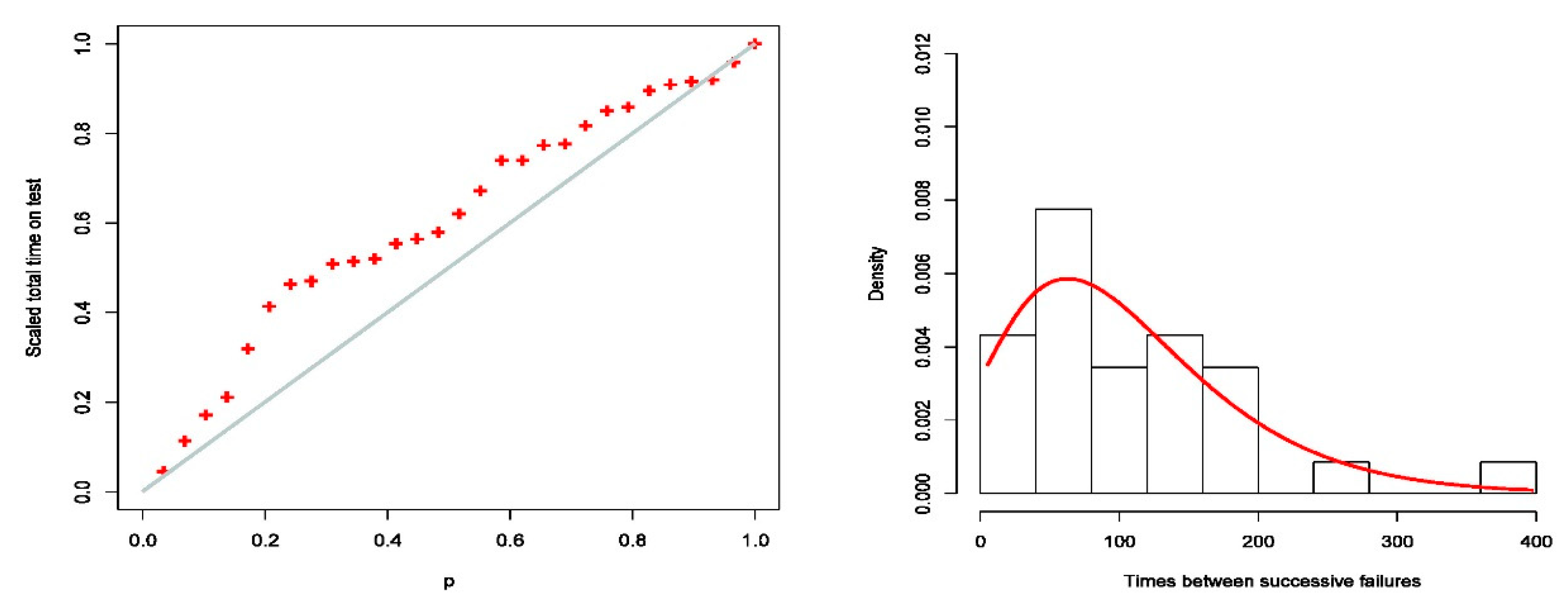
Total time on test time (TTT) is plotted in Figure 3 with an increasing FR function (left). The histogram of the data and the calculated PDF of the EQL are shown on the right.

The dataset was fitted to the EQL and some alternative models as a comparative analysis. The parameters of the EQL are estimated using the MLE and EM methods. The estimates from EM and ML are approximately the same. The alternative models include the gamma, exponentiated gamma (EG), Lehmann gamma (LG), Marshal-Olkin gamma (MOG), and QL. For each model, the Akaike information criterion (AIC), Cramer-von Mises (CVM) statistics, Anderson-Darling (AD) statistics, and Kolmogorov-Smirnov (KS) statistics are calculated and summarized in Table 3.

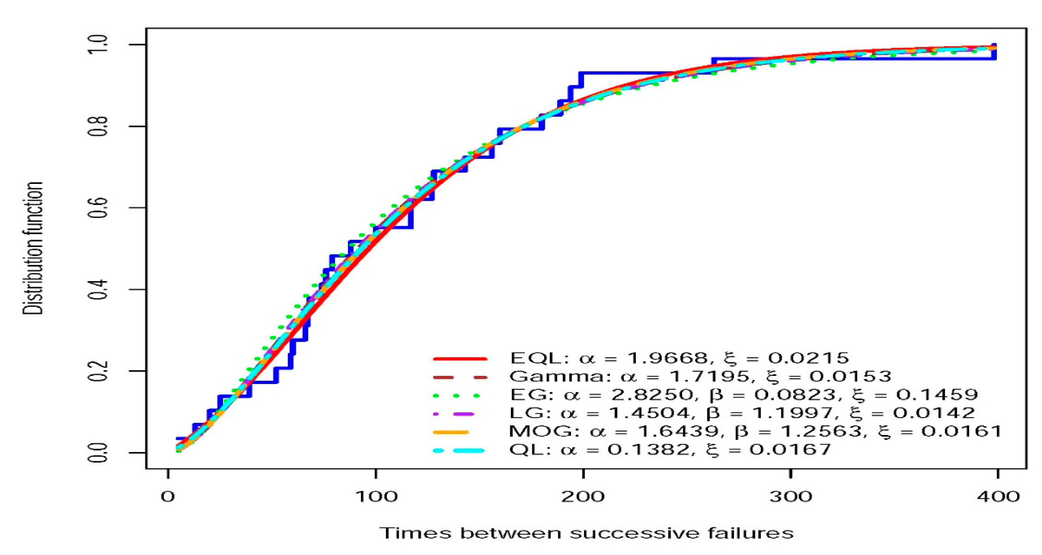
The analysis shows that the EQL performs better than the other models in all the statistics considered. In Figure 4, the empirical and fitted distribution function for EQL and some alternatives are plotted and provides a graphical investigation.

6. Conclusions

For data modeling and analysis, the right statistical model must be used to draw more accurate conclusions. The EQL model, which combines three gamma distributions, is an extension of QL, which can be used in various scientific disciplines. The model can be useful in practice, as shown by the analysis of a data set consisting of the intervals between successive air conditioning failures of a Boeing 720 aircraft. The ML approach and the EM algorithm provide accurate and consistent parameter estimates based on simulation results. However, the EM algorithm provides a more accurate approximation than the MLE.

Acknowledgments

This work is supported by Princess Nourah bint Abdulrahman University Researchers Supporting Project number (PNURSP2023R226), Princess Nourah bint Abdulrahman University, Riyadh, Saudi Arabia.

Conflicts of Interest

The authors declare no conflict of interest.

References

Lindley, D.V. Fiducial distributions and Bayes’ theorem. J. R. Stat. Soc. Ser. (Methodol.) 1958, 20, 102–107. [Google Scholar] [CrossRef]
Ghitany, M.E.; Atieh, B.; Nadarajah, S. Lindley distribution and its application. Math. Comput. Simul. 2008, 78, 493–506. [Google Scholar] [CrossRef]
Shanker, R.; Ghebretsadik, A.H. A New Quasi Lindley Distribution. Int. J. Stat. Syst. 2013, 8, 143–156. [Google Scholar]
Zakerzadeh, H.; Dolati, A. Generalized Lindley distribution. J. Math. Ext. 2009, 3, 13–25. [Google Scholar]
Shanker, R.; Shukla, K.K.; Shanker, R.; Leonida, T.A. A Three-Parameter Lindley Distribution. Am. J. Math. Stat. 2017, 7, 15–26. [Google Scholar]
Merovci, F.; Sharma, V.K. The Beta-Lindley Distribution: Properties and Applications. J. Appl. Math. 2014, 2014, 198951. [Google Scholar] [CrossRef]
Ibrahim, E.; Merovci, F.; Elgarhy, M. A new generalized Lindley distribution. Math. Theory Model. 2013, 3, 30–47. [Google Scholar]
Sankaran, M. The discrete poisson-Lindley distribution. Biometrics 1970, 26, 145–149. [Google Scholar] [CrossRef]
Ghitany, M.E.; Al-Mutairi, D.K.; Balakrishnan, N.; Al-Enezi, L.J. Power Lindley distribution and associated inference. Comput. Stat. Data Anal. 2013, 64, 20–33. [Google Scholar] [CrossRef]
Al-Mutairi, D.K.; Ghitany, M.E.; Kundu, D. Inferences on stress-strength reliability from Lindley distribution. Commun. Stat.-Theory Methods 2013, 42, 1443–1463. [Google Scholar] [CrossRef]
Zamani, H.; Ismail, N. Negative Binomial-Lindley Distribution and Its Application. J. Math. Stat. 2010, 6, 4–9. [Google Scholar] [CrossRef]
Al-babtain, A.A.; Eid, H.A.; A-Hadi, N.A.; Merovci, F. The five parameter Lindley distribution. Pak. J. Stat. 2014, 31, 363–384. [Google Scholar]
Ghitany, M.E.; Al-Mutairi, D.K.; Aboukhamseen, S.M. Estimation of the reliability of a stress-strength system from power Lindley distributions. Commun. Stat.-Simul. Comput. 2015, 44, 118–136. [Google Scholar] [CrossRef]
Abouammoh, A.M.; Alshangiti Arwa, M.; Ragab, I.E. A new generalized Lindley distribution. J. Stat. Comput. Simul. 2015, 85, 3662–3678. [Google Scholar] [CrossRef]
Ibrahim, M.; Singh Yadav, A.; Yousof, H.M.; Goual, H.; Hamedani, G.G. A new extension of Lindley distribution: modified validation test, characterizations and different methods of estimation. Commun. Stat. Appl. Methods. 2019, 26, 473–495. [Google Scholar] [CrossRef]
Marthin, P.; Rao, G.S. Generalized Weibull-Lindley (GWL) distribution in modeling lifetime Data. J. Math 2020, 2020, 1–15. [Google Scholar] [CrossRef]
Al-Babtain, A.A.; Ahmed, A.H.N.; Afify, A.Z. A new discrete analog of the continuous Lindley distribution, with reliability applications. Entropy 2020, 22, 1–15. [Google Scholar] [CrossRef] [PubMed]
Joshi, R.K.; Kumar, V. Lindley Gompertz distribution with properties and applications. Int. J. Appl. Math. Stat. 2020, 5, 28–37. [Google Scholar] [CrossRef]
Afify, A.Z.; Nassar, M.; Cordeiro, G.M.; Kumar, D. The Weibull Marshall and Olkin Lindley distribution: properties and estimation. J. Taibah Univ. Sci. 2020, 14, 192–204. [Google Scholar] [CrossRef]
Chesneau, C.; Tomy, L.; Gillariose, J.; Jamal, F. The Inverted Modified Lindley Distribution. J Stat. Theory Pract. 2020, 14. [Google Scholar] [CrossRef]
Algarni, A. On a new generalized lindley distribution: Properties, estimation and applications. PLoS ONE 2021, 16, 1–18. [Google Scholar] [CrossRef]
Shanker, R.; Mishra, A. A quasi Lindley distribution. Afr. J. Math. Comput. Sci. Res. 2013, 6, 64–71. [Google Scholar]
Kayid, M.; Nassr, S. Al-Maflehi, EM Algorithm for Estimating the Parameters of Quasi-Lindley Model with Application. Journal of Mathematics 2022, 2022, 1–9. [Google Scholar]
Kayid, M.; Alskhabrah, R.; Alshangiti, A.M. A New Scale-Invariant Lindley Extension Distribution and Its Applications. Mathematical Problems in Engineering 2021, 3747753. [Google Scholar] [CrossRef]
Alrasheedi, A. , Abouammoh, A. and Kayid, M. A new flexible extension of the Lindley distribution with applications. Journal of King Saud University – Science 2022, 34, 1–9. [Google Scholar] [CrossRef]
Titterington, D.M.; Smith, A.F.M.; Makov, U.E. Statistical analysis of finite mixture distributions; John Wiley and Sons: Chichester, U.K., 1985. [Google Scholar]
Ord, J.K. Families of frequency distributions; Charles Griffin: London, U.K., 1972. [Google Scholar]
Lai, C.D.; Xie, M. Stochastic Aging and Dependence for Reliability; Springer, 2006; ISBN 978-0-387-29742-2. [Google Scholar]
Wu, C.F.J. On the convergence properties of the EM algorithm. Ann. Stat. 1983, 11, 95–103. [Google Scholar] [CrossRef]
Proschan, F. Theoretical Explanation of Observed Decreasing Failure Rate. Technometrics 1963, 5, 375–383. [Google Scholar] [CrossRef]

Figure 1. The PDF (left) and FR (right) of EQL for some parameter values.

Figure 2. The MRL (left) and median residual life (right) of EQL for some parameter values.

Figure 3. The TTT plot (left) and histogram along with estimated PDF (right) of times between failures of air conditioning system.

Figure 4. The empirical and estimated CDF for QL and some alternative models of times between failures of air conditioning system.

Table 1. Simulation results for ML, LSE, AD and EM algorithm. The first and second lines of every cell corresponds to

α

and

ξ

respectively.

Table 1. Simulation results for ML, LSE, AD and EM algorithm. The first and second lines of every cell corresponds to

α

and

ξ

respectively.

		$n$
Method		80		150
	$α, ξ$	B	MSE	B	MSE
MLE	0.1, 0.1	0.2093 0.0221	0.1413 0.0015	0.1486 0.0166	0.0853 0.0010
	0.3, 0.5	0.1009 0.0415	0.1222 0.0209	0.0466 0.0168	0.0771 0.0133
	0.8, 1	0.0598 0.0029	0.1716 0.0326	0.0273 -0.0043	0.0948 0.0201
EM	0.1, 0.1	0.0833 0.0097	0.0377 0.0004	0.0463 0.0054	0.0126 0.0002
	0.3, 0.5	0.1346 0.0530	0.1095 0.0181	0.0807 0.0329	0.0554 0.0100
	0.8,1	0.1023 0.0223	0.1856 0.0299	0.0281 0.0015	0.0728 0.0156
LSE	0.1, 0.1	0.2350 0.0306	0.1970 0.0026	0.1734 0.0230	0.1185 0.0016
	0.3, 0.5	0.0906 0.0523	0.1726 0.0315	0.0466 0.0287	0.1083 0.0206
	0.8,1	0.0609 0.0075	0.2960 0.0500	0.0143 -0.0038	0.1085 0.0270
Weighted LSE (AD)	0.1, 0.1	0.0283 0.0097	0.0592 0.0009	0.0249 0.0084	0.0392 0.0006
	0.3, 0.5	-0.1116 -0.0233	0.1157 0.0211	-0.1373 -0.0367	0.0778 0.0121
	0.8,1	-0.3220 -0.1497	0.2795 0.0700	-0.2426 -0.1230	0.1963 0.0466

Table 2. Time interval between successive failures of air conditioner system of Boeing 720 aircraft.

10	60	186	61	49	14	24	56	20
84	44	59	29	118	25	156	310	76
44	23	62	130	208	70	101	208

Table 3. Fitting the successive times between failures.

Model	$\hat{α}$	$\hat{β}$	$\hat{ξ}$	AIC	CVM	AD	KS
					p-value	p-value	p-value
EQL	1.9668	—	0.0215	331.22	0.0278 0.9843	0.1833 0.9944	0.0801 0.9923
Gamma	1.7195	—	0.0153	331.55	0.0363 0.9539	0.2399 0.9754	0.1028 0.9190
EG	2.8250	0.0823	0.1459	334.57	0.0647 0.7882	0.3836 0.8638	0.1308 0.7037
LG	1.4504	1.1997	0.0142	333.59	0.0373 0.9682	0.2454 0.9727	0.1041 0.9120
MOG	1.6439	1.2563	0.0161	333.37	0.0322 0.9705	0.2169 0.9851	0.0965 0.9498
QL	0.1382	—	0.0167	331.35	0.0320 0.9712	0.2057 0.9888	0.0965 0.9499

Disclaimer/Publisher’s Note: The statements, opinions and data contained in all publications are solely those of the individual author(s) and contributor(s) and not of MDPI and/or the editor(s). MDPI and/or the editor(s) disclaim responsibility for any injury to people or property resulting from any ideas, methods, instructions or products referred to in the content.

© 2023 by the authors. Licensee MDPI, Basel, Switzerland. This article is an open access article distributed under the terms and conditions of the Creative Commons Attribution (CC BY) license (http://creativecommons.org/licenses/by/4.0/).

Copyright: This open access article is published under a Creative Commons CC BY 4.0 license, which permit the free download, distribution, and reuse, provided that the author and preprint are cited in any reuse.

MDPI Initiatives

Important Links

Choose an area of interest and we will send you notifications of new preprints at your preferred frequency.

Disclaimer

10	60	186	61	49	14	24	56	20
84	44	59	29	118	25	156	310	76
44	23	62	130	208	70	101	208

10	60	186	61	49	14	24	56	20
84	44	59	29	118	25	156	310	76
44	23	62	130	208	70	101	208

Scaled-Invariant Extended Quasi-Lindley Model: Properties, Estimation and Application

Abstract

1. Introduction

2. Scaled-invariant extended QL model

2.1. Statistics and Reliability Properties

3. Estimation

3.1. ML method

3.2. LSE method

3.3. Weighted LSE method

3.2. EM algorithm

4. Simulations

5. Application

6. Conclusions

Acknowledgments

Conflicts of Interest

References

MDPI Initiatives

Important Links

Subscribe

10	60	186	61	49	14	24	56	20
84	44	59	29	118	25	156	310	76
44	23	62	130	208	70	101	208