Preprint
Article

A Novel Hybrid Optimization Approach for Fault Detection in PV Arrays and Inverters Using AI and Statistical Learning Techniques: A Focus on Sustainable Environment

Altmetrics

Downloads

167

Views

44

Comments

0

A peer-reviewed article of this preprint also exists.

Submitted:

24 July 2023

Posted:

25 July 2023

You are already at the latest version

Alerts
Abstract
Fault detection in PV arrays and inverters is critical for ensuring maximum efficiency and performance. Artificial intelligence (AI) learning can be used to quickly identify issues, resulting in a sustainable environment with reduced downtime and maintenance costs. As the use of solar energy systems continues to grow, the need for reliable and efficient fault detection and diagnosis techniques becomes more critical. This paper presents a novel approach for fault detection in photovoltaic (PV) arrays and inverters, combining AI techniques. It integrates Elman Neural Network (ENN), Boosted Tree Algorithms (BTA), Multi-layer Perceptron (MLP), and Gaussian Processes Regression (GPR) for enhanced accuracy and reliability in fault diagnosis. It leverages their strengths for accuracy and reliability of fault diagnosis. Feature engineering-based sensitivity analysis was utilized for feature extraction, the fault detection and diagnosis were assessed using several statistical criteria including PBAIS, MAE, NSE, RMSE, and MAPE. Two intelligent learning scenarios are carried out, the first scenario is done for PV array fault detection with DC power (DCP) as output. The second scenario is done for inverter fault detection with AC power (ACP) as the output. The proposed technique is capable of detecting faults in PV arrays and inverters, providing a reliable solution for enhancing the performance and reliability of solar energy systems. Real-world solar energy dataset is used to evaluate the proposed technique, with results compared to existing detection techniques and obtained results show that it outperforms existing fault detection techniques, achieving higher accuracy and better performance. The GPR-M4 optimization justified reliably among all the models with MAPE=0.0393, and MAE=0.002 for inverter fault detection and MAPE=0.091, and MAE=0.000 for PV array fault detection.
Keywords: 
Subject: Engineering  -   Electrical and Electronic Engineering

1. Introduction

Advancement in renewable energy technology has been on a rapid ascending trend in recent years. This has encouraged wide acceptance of the technology and thus, the subsequent boom in the installation of renewable energy-based power plants around the world especially in China, India, Europe and America. Solar photovoltaic (PV) is one of the leading renewable energy technologies on exponential rise. Due in part to the growing concern over oil depletion, environmental issues, fuel price dependence, and operational complexity associated with the production of fossil fuels, an increasing number of residential, commercial, and industrial consumers have adopted and are adopting solar PV as their source of power generation [1]. The National Renewable Energy Lab (NREL) reported that the PV capacity installed globally in 2021 was 172GWdc bringing the global cumulative capacity to 939GWdc [2]. NREL further stated that China, India and Germany significantly increased their PV installations by 106%, 51% and 22% respectively, in the first 9 months of 2022 [3]. This remarkable rise in the significance of solar PV in the global energy sector is also reflected in [2], where it is reported an increased annual global PV installations especially in the aforementioned countries was projected by analysts.
However there are is a downside to the technology. Solar PV systems require ongoing maintenance in order to function efficiently over time because they have been known to lose efficiency and productivity if not properly and appropriately managed and maintained [1]. That is to say, in order for solar PV systems to operate properly over time, they need to undergo routine maintenance, which calls for the adoption of mechanisms to efficiently monitor and control these systems. Several operation and maintenance conventional methods which have helped to sustain efficient operation of PV systems have been introduced over the years. These methods however have not been able to totally prevent system failure and operation downtime which begs the need for more intelligent methods of fault detection and the subsequent adoption of AI-based methods. These techniques make use of machine learning to develop models that can quickly find various issues, track the overall health of PV systems, and assist maintenance engineers in hastening system recovery [4].
There are so many available literatures that have carried out experiments and researches on the use of AI in fault detection and diagnosis for PV systems. In [5], a straightforward and efficient monitoring technique for PV systems is given. It is based on parametric models and the double exponential smoothing scheme. In order to find minor deviations, the simplicity and adaptability of empirical models are combined with the sensitivity of a double exponential smoothing method. By analyzing the resulting residuals, the double exponential smoothing approach detects flaws, and its sensitivity is increased by creating a nonparametric detection threshold using kernel density estimation. Partial shading, inverter disconnections, PV string faults, soiling on PV arrays, and short circuits in PV modules are just a few of the defects that can be found utilizing the suggested method. The research's findings, demonstrated that the suggested method can be used to monitor PV system operating parameters in real-time but may not be suitable for spotting abnormalities at various scales because it was designed for one scale, namely the time scale. By implementing grid partition (GP) and subtractive clustering (SC) algorithms utilizing research data, the approach suggested in [6] trains the adaptive neuro-fuzzy inference system (ANFIS) model for a reliable PV defect detection and classification system. Afterwards, in order to identify PV system problems, the trained models ANFIS GP and ANFIS SC were used. The resulting data were compared using statistical analysis. It was discovered that in terms of precisely identifying fault states, the ANFIS SC technique outperformed the ANFIS GP technique. The proposed method may not be appropriate for the identification of faults in various PV systems where the environmental factors are beyond the specified model range, according to the authors, who also emphasized that the method solely considers electrical defects. Using thermographic pictures, a fault detection technique is provided in [7] that categorizes various PV module anomalies. A multi-scale convolutional neural network (CNN) with three branches is used in the technique, which is based on the transfer learning approach. The transferred network's pre-trained information is used in the convolutional branches, which also have multi-scale kernels with levels of visual perception, to enhance the network's capacity for representation. By combining an oversampling strategy with an offline augmentation method, the study was able to improve network performance while overcoming the unbalanced class distribution of the raw data.
The suggested method was used in the experiment to identify a variety of fault kinds, and the study came to the conclusion that it performs better than other deep learning methods and studies now available and provides higher classification accuracy and robustness in PV panel defects. Thermographic images are used in yet another technique described in [8] to identify flaws in PV systems. Here, deep convolutional neural networks (DCNNs) and infrared thermographic images are used together to detect and diagnose faults. The method involves first creating a binary classifier to identify faults in PV modules, then creating a multiclass classifier to determine what kind of flaws are there. The study takes into account four typical PV module faults: short-circuiting, partial shading effects, dust deposition on PV module surfaces, and bypass diode failure. The proposed DCNN-based classifiers have been first optimized, then embedded into a low-cost microprocessor (Rasberry Pi 4), and the models are compared with three main TF-Lite optimization strategies, including simple conversion, dynamic range quantization, and float 16 quantization. The study came to the conclusion that the proposed technique can operate in real-time and can diagnose and detect anomalies with a level of accuracy that is acceptable based on the experimental findings that were obtained. Additionally, the technique is set up to send email and SMS using a GSM module to operators informing them of the status of the PV array. The authors of Study [9], which also presents a thermographic image-based method, noted that it is crucial to quickly and affordably maintain the proper functioning of PV systems without interrupting regular operations by identifying PV module overheating through thermographic non-destructive testing. The paper then suggested a technique for convolutional neural networks that was created using open-source libraries to automatically classify thermographic images. To lower image noise, a number of preprocessing techniques were tested, including grey-scaling, thresholding discrete wavelet transform, normalizing and homogenizing pixels, normalizing and homogenizing pixels, Sobel Feldman and box blur filtering, and thresholding discrete wavelet transform. Without following any set protocols, these techniques enable the classification of thermographic images of varying quality that are taken using various pieces of equipment. The performance of neural networks was evaluated using the suggested method through a number of experiments using various parameters and overfitting mitigation techniques. In order to assess network performance and the amount of time needed to complete the thermographic inspection, images obtained by unmanned aerial vehicles and ground-based operators were compared. The foundation of the proposed method is a tool built on convolutional neural networks that enables rapid and accurate failure detection in PV panels.
According to the authors, the proposed methodology provides an alternative and a reliable tool that enhances the resolution of picture classification for issues involving remote failure detection and can be applied in any field of science. Study [10] provides a summary of IoT and AI applications for PV systems. The most cutting-edge algorithms, including machine and deep learning, are also discussed in the paper, along with their implementation costs, accuracy, complexity, software appropriateness, and viability for real-time applications. For PV facilities located in remote locations with expensive and difficult accessibility for maintenance, the integration of AI and IoT approaches for defect detection and diagnosis into basic hardware such as inexpensive chips, may be economically and technically possible. These strategies were also provided together with challenging problems, advice, and trends. In [11], a study examining the use of ANN in various areas of partially shaded PV systems is provided. It provided an overview of and covered the use of ANNs in MPPT, fault detection, fault mitigation, system modeling, and performance enhancement of solar PV systems exposed to partial shading. The study did not just examine the literature; it also showed how the approaches may be enhanced and applied in real-world settings. The study described in [12] assesses various ML and ensemble learning (EL) algorithms for fault diagnosis of PV arrays, including previously untested methods for faults with numerous faults and faults with comparable I-V curves. The study created a novel method to accurately identify and classify defects based on this evaluation. According to the authors' findings, the results are positive. The study went further to demonstrate when ML & EL methods ought to be applied in practice and provided some recommendations, difficulties, and potential future directions in this area. By suggesting an early degradation detection that affects glass, EVA, wiring, etc., the work described in [13] aims to lower operation costs of PV modules. In the suggested approach, automated self-evaluation of PV panels is created, and degradation models are integrated as software into a microcontroller that uses instantly measured parameters. In the study, it is also discussed the deterioration phenomena of each PV module's component. Modeling each recognized degradation using P-V characteristics is the basis for the Observing Degradation System (ODS) program, which is then presented. A checklist is then created for successful testing. Study [14] presents an ensemble-based deep neural network (DNN) model for the autonomous detection of visual faults on various PV modules, including glass breakage, burn marks, snail trails, discoloration, and delamination. This method for detecting degradation faults is similar to the one described earlier. A RGB camera placed on an unmanned aerial vehicle is used in the procedure to capture the image dataset (UAV). Images are preprocessed by removing spatial and frequency domain characteristics from them, such as discrete wavelet transform, texture grey level co-occurrence matrix, rapid Fourier transform, and different grey level approach. Following that, the edited photos are input. To identify any visual defects on the PV modules, the proposed ensemble-based DNN model uses DNN. In order to assess the performance of the suggested model, the classification accuracy, receiver operating characteristic curve, and confusion matrix are utilized. The results revealed that the proposed model, coupled with random forest classifier, achieved a high classification accuracy.
Similarly, in [15], the authors described a fuzzy diagnostic algorithm that relies on the classification of electrical characteristics, the values of which are taken from experimental measurements of crystalline modules' I-V curves. By using the suggested method, flaws like uniform dust, partial shading, and potential induced degradation can be found. Also, a brand-new approach is suggested for the detection of aberrations in the measured I-V curve brought about by bypasses that are activated as a result of partial shading. This is based on quadratic and cubic polynomial regression, whose concavities are very sensitive to noisy data. An approach for identifying, diagnosing, and categorizing short-circuit and open-circuit string errors that is based on deep learning is provided [16]. There are four steps in the suggested technique. First, a PSIM-based simulation that seeks to accurately represent the functioning PV system using a heuristic optimization approach based on the Coyote Optimization Algorithm (COA) is used to input five unknown electrical characteristics of one diode model. The second phase involves creating a database with information on current, voltage, and power at MMP, module temperature, and solar irradiation for the PV system under both ideal and unsatisfactory working circumstances. In the third stage, new features from the old database are extracted using the unsupervised learning capabilities of the auto-encoder, and in the final step, PV defect detection and classification are accomplished using supervised learning on the new database based on ANN construction. The obtained results show how well the suggested strategy works with the aforementioned fault kinds. Study [17] investigates the effects of various physical faults and cyberattacks in order to develop an intelligent fault/attacks detection and diagnosis system. They find that by being able to quickly identify and diagnose fault/attacks, local controllers and energy management systems can accommodate or lessen the negative effects of physical faults and cyberattacks in microgrids. The study then presented an intelligent hybrid diagnosis method for data online monitoring and diagnosing to reflect the real-time state of PV system running at microgrid level. The proposed method is based on a fuzzy inference system, a power spectrum estimator, and an adaptive neuro-fuzzy inference system. A realistic microgrid benchmark model with a range of operating conditions and dynamic electrical loads in the presence of potential microgrid disturbances is used to show the high level of efficiency of the proposed method under various types of fault/attack scenarios. In [18], a fault detection and diagnosis (FDD) scheme design is presented that employs Wasserstein generative adversarial network (WGAN) and convolutional neural network for automatic fault feature extraction from raw electrical data of PV array, resulting in the creation of an effective FDD model with little data. A classifier, a generator, and a discriminator make up the three modules that make up the FDD model. In order to enhance the effectiveness of the CNN-based classifier, the discriminator and generator analyze sequential PV data in a two-dimensional manner to learn the distribution of PV data under different PV system operations. Then they are utilized to generate additional labelled data samples. According to the paper, the suggested FDD model could be trained with only a little amount of labeled data, and the effectiveness of the model was assessed using a lab grid-connected PV setup.
A diagnosis of line-line and open-circuit faults using the suggested method was demonstrated by the results. An implementation of a fault detection strategy based on the identification of PV systems' neuro-fuzzy models is presented in the work in [19]. Modeling and identification of systems and the detection of operational states are the two stages of the technique. The derived neuro-fuzzy model approximates, with only a few minor differences, the properties and behavior of a genuine system. The suggested model has a very high level of accuracy and could identify errors very quickly. Three shortcomings in machine learning-based defect detection techniques were listed in Study [20], which is what it seeks to fix. The inability of shallow network structures to effectively learn nonlinear characteristics of I-V curves is one of them. The others are that feature extraction relies on expert experience and lacks automation; artificial feature extraction readily ignores some potentially useful features; and feature extraction is not automated. As a result, the study suggested a methodology based on layered automated encoder and clustering algorithm that can automatically extract features and employ a limited amount of labeled data samples to mine data sample characteristics for defect diagnosis. Three steps make up the technique's execution. To enhance the effectiveness of the clustering approach, the effective features are first automatically retrieved from the I-V curves by the stacking encoder, and then the dimension of the features is decreased and visualized by the t-distributed stochastic neighbor embedding. Eventually, the clustering method produces clustering centers and clusters, and the membership function is utilized to diagnose faults. Eventually, the clustering method produces clustering centers and clusters, and the membership function is utilized to diagnose faults. To address the issue of fault detection of PV modules using thermographic images, a Convolutional Neural Network (CNN) model and a fine-tuned model based on Visual Geometry Group (VGG-16) have been investigated in [21]. Binary classification and multiclass classification were employed to determine the type of fault in order to detect it. The database utilized in the study was made up of an unbalanced class distribution of thermographic images taken by infrared cameras of PV modules both in good and bad condition (such as bypass diode failure, partially covered PV module, shading effect, short-circuit and dust deposit on the PV surface). The fine-tuned model performs very well in experimental tests, but the small Deep Convolutional Neural Network (small-DCNN) model performs somewhat less well.
This study presents a novel method of fault detection in PV arrays and inverter faults by utilizing Elman Neural Network (ENN), Boosted Tree Algorithms (BTA), Multi-later Perceptron (MLP) and Gaussian Processes Regression (GPR) models to estimate the DC Power (DCP) and AC Power (ACP) of a PV system setup. Different models have different strengths and weaknesses, and what works well for one problem may not work as well for another. Therefore, it is important to experiment with different models and choose the one that is best suited for the particular task at hand [22]. As such, we develop several model combination based on the influencing factors (see Figure 2), existing claimed of dominancy in the literature [23,24,25,26]. Furthermore, it is important to evaluate the performance of the chosen model carefully, using appropriate metrics and validation techniques, to ensure that it is indeed performing well on the given problem. As such the study employs several performance criteria to assess the accuracy of the models. Prior to model development, data pre-processing including normalization, model validation and stationarity analysis, is carried out. Also, both standalone and hybrid models will be compared using Nash–Sutcliffe efficiency (NSE), Pearson correlation coefficient (PCC), mean absolute percentage error (MAPE), mean absolute error (MAE), root mean square error (RMSE), and Percent bias (PBAIS) to understand the strength of each model combination.

2. Components Methodology

2.1. DC Power

Solar panels use PV technology to turn sunlight into DCP. It is a kind of electricity that only goes in one direction. Only Batteries and DC loads are powered by DCP. To power AC loads, DCP must first be converted to ACP using an inverter. Majority of electrical appliances and equipment in houses and buildings operate on ACP.

2.2. AC Power

In order to power appliances, lighting, and other electrical loads in homes and businesses, AC electricity is typically employed. ACP is a type of electrical current that has a sinusoidal waveform and goes back and forth. Inverters are used to convert DC electricity produced by solar panels into ACP, which may subsequently be utilized to power AC loads.

2.3. Daily Yield

The amount of electricity produced by a solar panel system in a single day is referred to as daily yield. It is commonly expressed in kilowatt-hours (kWh) and is influenced by things like the size of the solar panel system, how effective the panels are, and how much sunlight is available during the day. A solar panel system's daily yield can be used to predict how much energy it will produce over time and to assess its financial return on investment.

2.4. Ambient Temperature

The term "ambient temperature" describes the temperature of the environment or the air around you. When it comes to solar energy, the ambient temperature can have an impact on how well solar panels work because hotter temperatures can reduce panel output and efficiency. When building and installing solar panel systems, it's crucial to take the ambient temperature into account as solar panels perform better at lower temperatures.

2.5. Module Temperature

The temperature of the solar panels itself is referred to as the module temperature. Solar panels may get fairly hot as they collect sunlight, which may have an impact on how well they work. The output and efficiency of panels may decline as module temperatures rise. Solar panels are frequently mounted with a space between the panel and the mounting surface to allow for air circulation in order to minimize overheating.

2.6. Solar Radiation

The energy that the sun emits and that reaches the earth is referred to as solar radiation. It consists of infrared (IR), ultraviolet (UV), and visible light (light). Solar panels use sun radiation as its energy source in order to produce electricity. Solar radiation received by solar modules vary based on its location, the time of day, the season, and the weather. The energy output of a solar panel system is calculated using the intensity of solar radiation, which is commonly expressed in terms of watts per square meter (W/m2).

3. Proposed Intelligent Methods

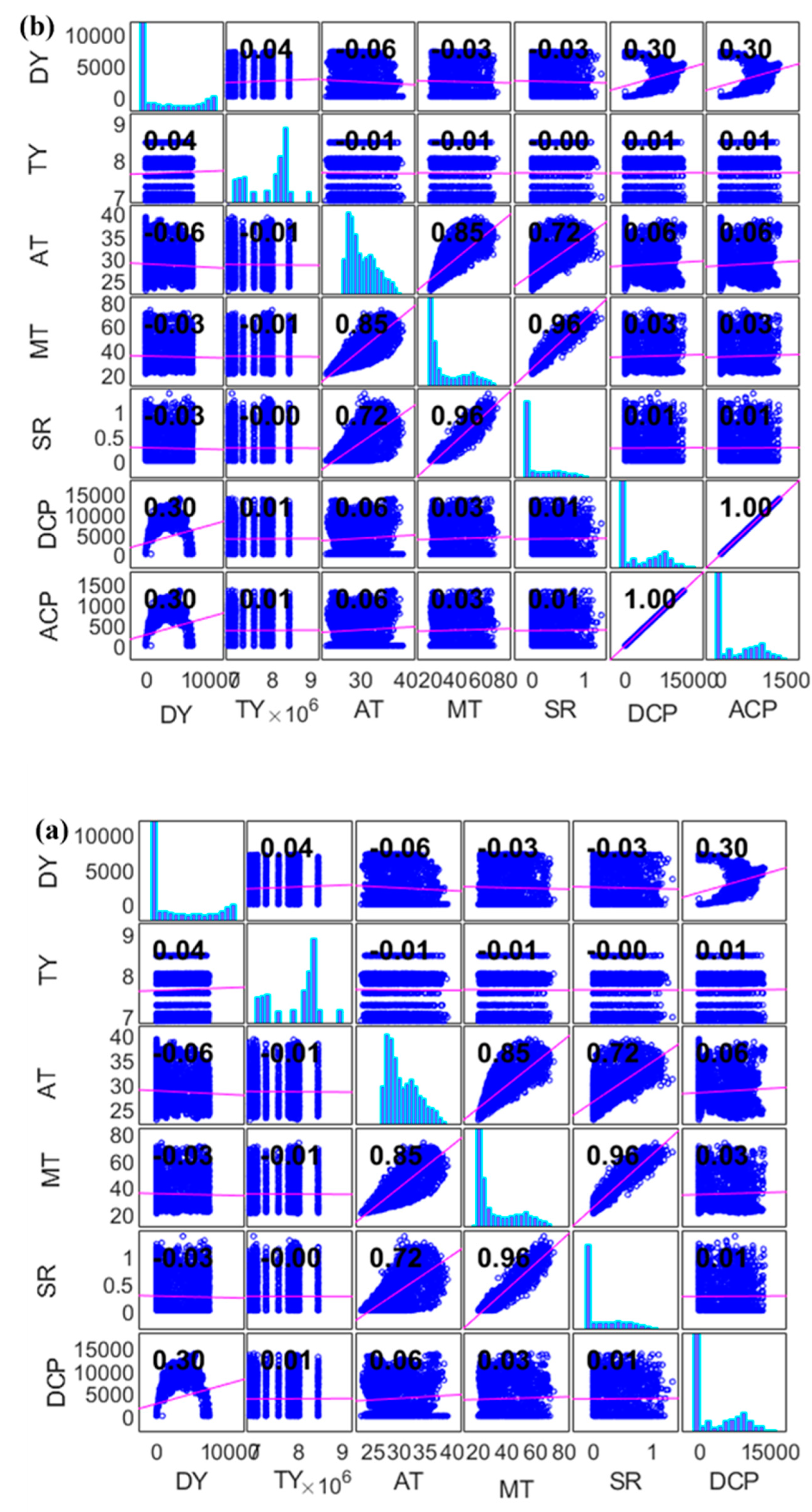
According to the “no free lunch" theorem, there is no single model that is universally better than all other models for every type of problem. In other words, there is no one-size-fits-all model that can provide optimal results across all possible scenarios [27]. In this work we proposed several AI learning based on three different scenarios (cropland, pasture, and cropland and pasture) to estimate the DCP and ACP based on solar panel and inverter, respectively. For this purpose, ENN, BTA, MLP and GPR models are utilized. The proposed modeling schematics is presented in Figure 1. It is essential to consider the specific characteristics of the problem at hand, such as the nature of the data, the size of the dataset, and the goals of the analysis. Different models have different strengths and weaknesses, and what works well for one problem may not work as well for another. Therefore, it is important to experiment with different models and choose the one that is best suited for the particular task at hand [22]. As such we developed several model combinations based on the influencing factors (see Figure 2), existing claimed of dominancy in the literature [23,24,2526] as follows:
S o l a r   P a n e l   ( D C P ) = M 1 = Φ D Y + A T + M T M 2 = Φ D Y + A T + M T + S R + T Y
I n v e r t e r   ( A C P ) = M 1 = Φ D C P M 2 = Φ D Y + A T + M T M 3 = Φ D Y + A T + M T + S R + T Y M 4 = Φ R D Y + A T + M T + S R + T Y + D C P
Where, DCP is DC Power, ACP is AC Power, DY is Daily Yield, AT is Ambient Temperature, MT is Module Temperature, and SR is Solar Radiation.
Furthermore, it is important to evaluate the performance of the chosen model carefully, using appropriate metrics and validation techniques, to ensure that it is indeed performing well on the given problem. As such this study employed several performance criteria to assess the accuracy of the models. Prior to model development, several pre-processing including normalization (Equation (3)), model validation and stationarity analysis, were carried out. In this study, both the standalone and hybrid models were compared using NSE (Nash–Sutcliffe efficiency), PCC (Pearson correlation coefficient), MAPE (mean absolute percentage error), MAE (mean absolute error), RMSE (root mean square error), and PBAIS to understand the strength of each model combination.
y = 0.05 + 0.95 x x ¯ x m a x + x m i n
Where y denotes normalized data, x is the actual data, x ¯ is the mean of the measured data, xmax denotes the maximum value of the measured data, and xmin denotes the minimum value.
N S E = 1 i = 1 N ( Y p Y ( o ) ) 2 i = 1 N ( Y p Y ( o ) ) 2
P C C = i = 1 N Y o , i Y ( p ) ¯ Y ^ o , i Y ~ ( p ) i = 1 N Q Y o , i Y ( p ) 2 Y ^ o , i Y ~ ( p ) 2
R M S E = 1 N i = 1 N ( Y p Y ( o ) ) 2
M A E = i = 1 N Y ( p ) Y ( o ) N
M A P E = 100 n i = 1 N Y ( o ) Y ( p ) Y ( o )
P B I A S = i = 1 N ( Y ( o ) Y ( p ) ) i = 1 N Y ( p ) )
Where by;   Y   p , Y ( o ) ,   Y o ¯ are considered as the TP loss rate predicted, Y ( o ) observed and Y o ¯ average values respectively.

3.1. Elman Neural Network (ENN)

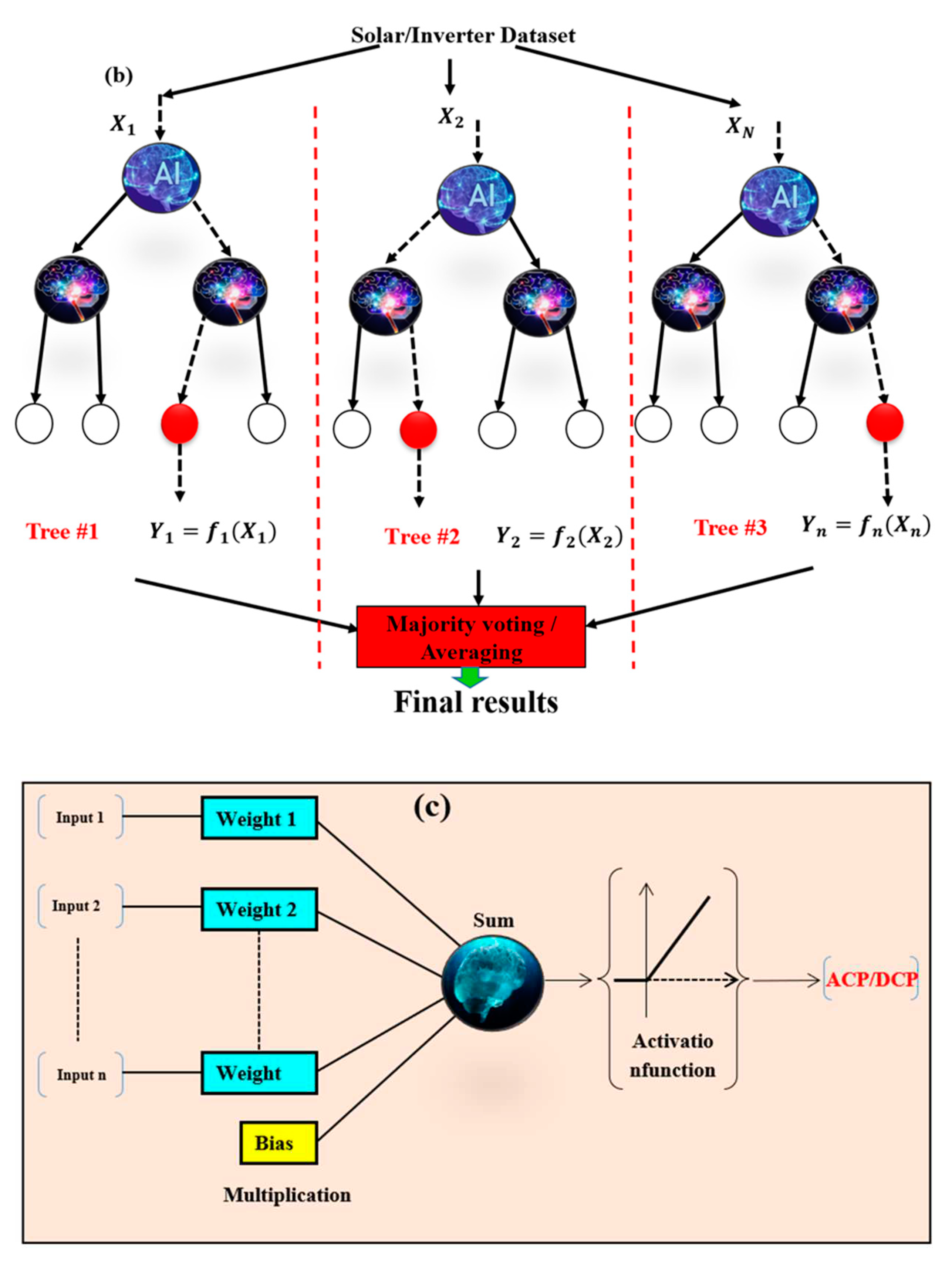
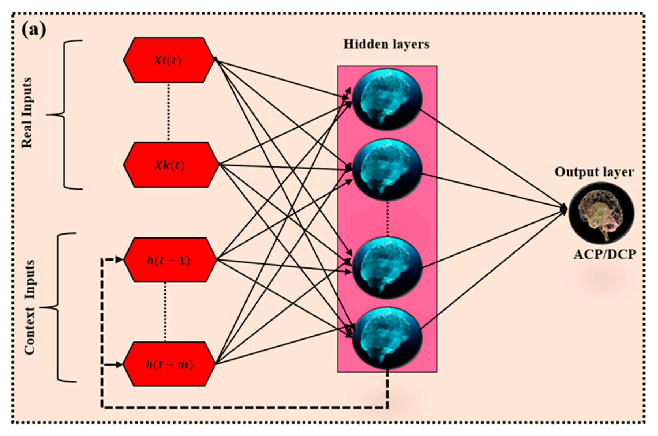
As recurrent computational learning, ENN is a type of machine learning technique that uses feedback connections to retain information about previous inputs. It comprises of different three layers as presented in Figure 2a similar to traditional neural network with the hidden layer having additional connections to itself from the previous time step [28]. This allows the network to capture sequential information and make predictions based on past inputs. The network is trained using backpropagation through time, where the error is propagated through the network and the weights are updated accordingly [29]. The ENN has been used in numerous purposes, both in science and engineering problems [30,31].

3.2. Boosted Tree Algorithms (BTA)

BTA are machine learning techniques that combine multiple decision trees to create a powerful predictive model (Figure 2b). The term "boosting" refers to the process of iteratively improving the performance of the model by focusing on the misclassified instances in each iteration. Boosted trees can be applied to both supervised and unsupervised learning problems [32]. The most popular boosted tree algorithms are Gradient Boosted Trees (GBTs) and Extreme Gradient Boosting (XGBoost). These algorithms work by sequentially adding trees to the model, with each subsequent tree trying to correct the errors made by the previous ones. The projection is obtained by aggregating the predictions of all the trees [33]. GBTs and XGBoost have several hyperparameters that can be tuned to optimize performance, including the learning rate, number of trees, tree depth, and regularization. These algorithms have been successfully applied in various domains, including finance, e-commerce, and healthcare. They are known for their high accuracy and interpretability, as they provide information on the importance of each feature in the prediction [32,34].

3.3. Multi-later Perceptron (MLP)

As another version of ANN, MLP model consists of multiple layers of interconnected perceptron units. MLP plays the role of FFNN in terms of information processing through the three layers (input, hidden, and outputs) [35] (Figure 2c). Each layer contains one or more nodes (perceptrons) that receive input from the previous layer and produce an output that is transmitted to the next layer [36]. The perceptrons in the hidden layers use activation functions to transform the inputs, allowing the network to learn complex mapping in the data. The MLP is trained using a supervised learning approach called backpropagation, hence works based on the principle of reducing the error between the estimated and observed data [37].

3.4. Gaussian Processes Regression (GPR)
GPR model has been used to solve different problems related to regression analysis in both science and engineering [38]. It uses Bayesian inference to make predictions and estimate uncertainties in the predictions. In contrast to other regression models, GPs do not make assumptions about the underlying function that generates the data, making them more flexible and suitable for modeling complex, nonlinear relationships. The core idea behind GPR is to assume that the function values at any set of input points are jointly Gaussian distributed [39]. A GP is defined by a mean function and a covariance function, also called the kernel function. The mean function specifies the expected value of the function at any input point, while the kernel function captures the similarity between different input points [40,41].
Figure 2. Schematic diagram of (a) ENN (b) BTA (c) MLP used in modelling process.
Preprints 80376 g002aPreprints 80376 g002b

4. Application of Results and Discussion

In this section the modelling results for two different scenarios were discussed based on solar panel (DCP) and inverter (ACP) modelling. It is worth to note that the use of AI models to simulate and optimize the performance of solar photovoltaic power plants is a novel approach that allows for better prediction and control of energy production, leading to increased efficiency and cost-effectiveness.

4.1. Preliminary Results

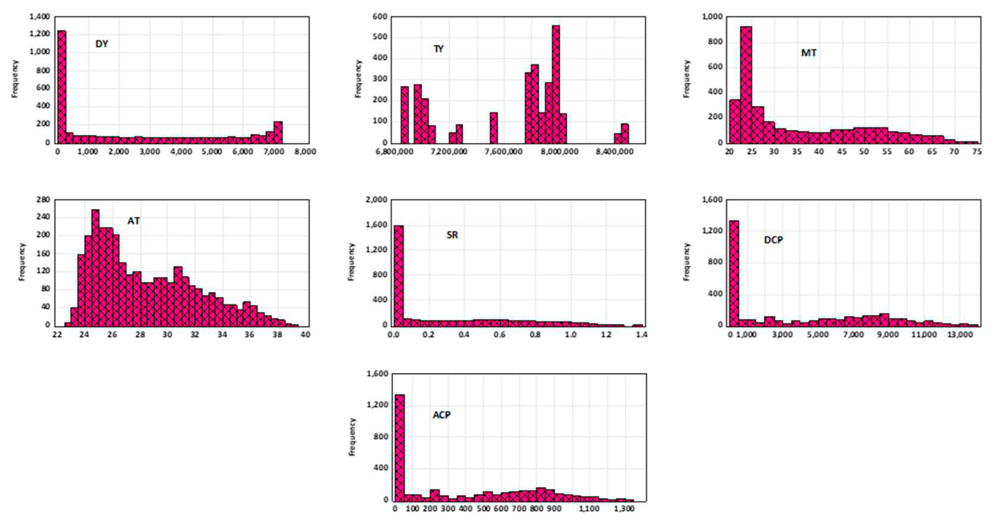
According to [42], to understand the model performance or on the other hand, the model to perform at its best, it is essential to include all factors associated with the removal process of HMs in the input data optimization. This step will enhance the output and ensure that the model's results align as closely as possible with the experimental data. Descriptive statistics and raw data analysis are crucial in modeling because they provide a comprehensive understanding of the data's characteristics and patterns. Table 1 shows the input-output descriptive analysis. This information can guide the selection of appropriate modeling techniques, the validation of model assumptions, and the interpretation of model results, leading to more accurate and reliable predictions. The time series data used in this study can be visualized in Figure 3.
The table presents descriptive statistics for six parameters: DY, TY, AT, MT, SR, DCP, and ACP. The Kurtosis column represents the peakness of the distribution, with a negative value indicating a flatter distribution than a normal distribution, and a positive value indicating a more peaked distribution. The Skewness column shows the degree of asymmetry in the distribution, with a negative value indicating a left-skewed distribution, and a positive value indicating a right-skewed distribution. The parameter TY has a Mean of 7,620,392.92 and an SD of 451,795.89, indicating that the data has a relatively high degree of variability. The Kurtosis value of -1.05 suggests that the distribution is relatively flat compared to a normal distribution. The Skewness value of -0.45 suggests that the data is slightly left-skewed. Finally, the Minimum and Maximum values of 6,870,716.67 and 8,460,553.49, respectively, show the range of observed values for the parameter. Similarly, the parameter with the lowest Kurtosis value is ACP with -1.21, while the parameter with the highest Kurtosis value is SR with -0.21. The parameter with the highest range of values is DCP, with a range of 13,687.94, while the parameter with the lowest range of values is SR, with a range of 1.36. According to [43,44,45,46,47], the lowest skewness towards negatives values indicated the feasibility of AI based learning in modelling the data accurately. The corro-plot as displayed in Figure 4 was used for input combination in this study. It can be seen that the system is highly stochastic approach based on the magnitude in Figure 4.

4.2. Results of Intelligent Leaning-Scenario I

In this section, modelling of solar panel as scenario-I was discussed based on the DCP (kW) parameter as output of the simulation. Table 2 represents the performance metrics of different models during the calibration phase. The models are evaluated using various metrics such as NSE, PCC, RMSE, MAPE, MAE, and PBIAS for both calibration and verification. From the results it can be observed that BTA-M1 and BTA-M2 show relatively good performance with NSE values of 0.914 and 0.921, respectively. They also have high PCC values of 0.967 and 0.97, indicating a strong linear relationship between the observed and predicted values. However, they have relatively high MAPE values of 35.267 and 33.745, indicating a higher average percentage difference between the predicted and observed values. Similarly the new recurrent approach i.e. ENN-M1 and ENN-M2 exhibit even better performance, with NSE values of 0.973 and 0.971, respectively, indicating a high degree of agreement between the observed and predicted values. They also have high PCC values of 0.99 and 0.989, indicating a strong linear relationship between the observed and predicted values. Additionally, ENN-M1 and ENN-M2 have low RMSE values of 0.045 and 0.047, respectively, indicating a lower overall error compared to the other models.
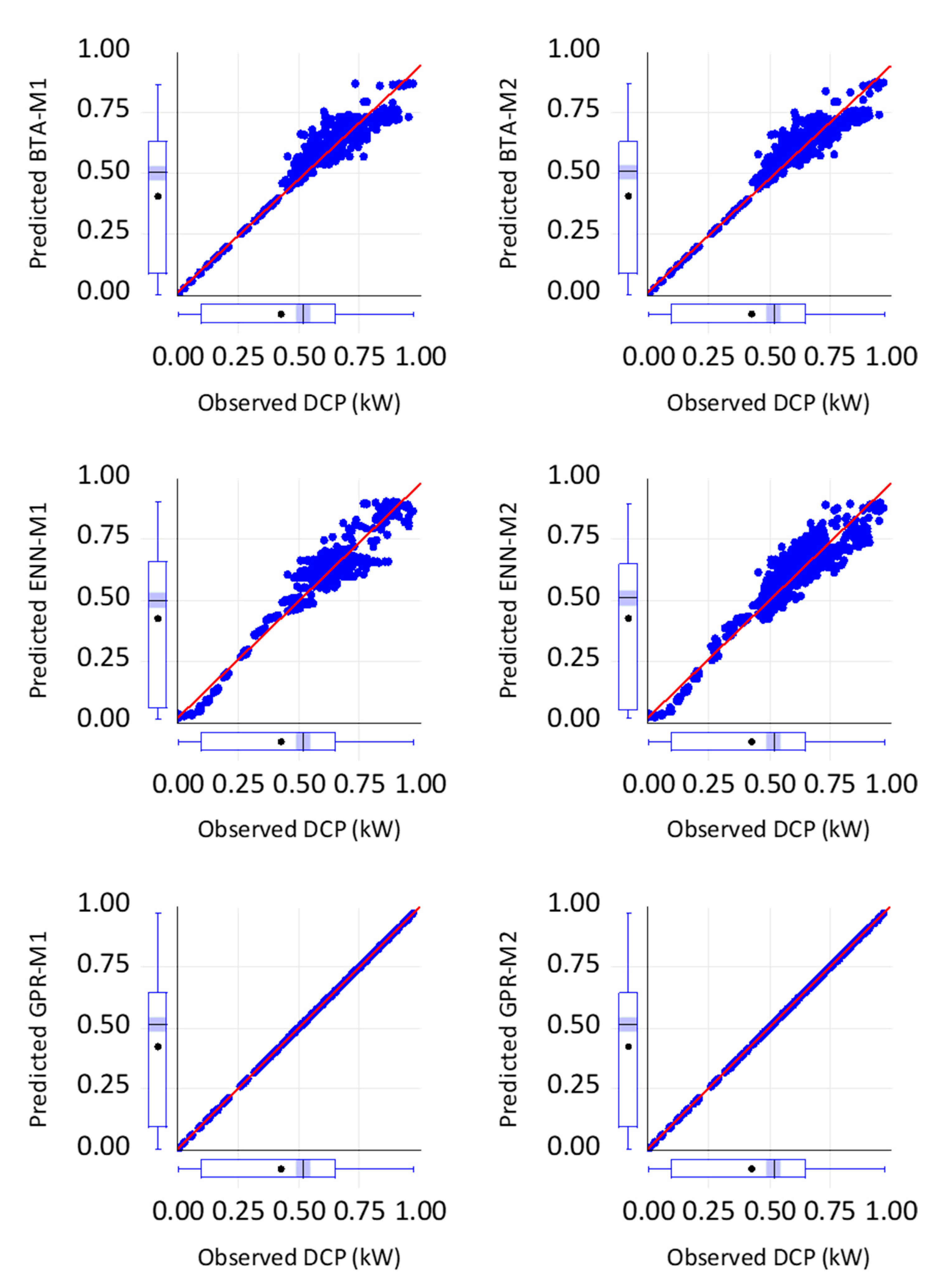
However, they have a negative PBIAS value, indicating a tendency to under-predict the observed values. GPR-M1 and GPR-M2 show perfect correlation (PCC value of 1) and no error (RMSE value of 0), making them the best-performing models. However, GPR-M2 has a slightly higher MAE value of 0.001 compared to GPR-M1, which has an MAE value of 0. Overall, the table provides a good summary of the performance of different models during the calibration phase. It helps in evaluating the accuracy of predictive models and selecting the best model based on the evaluation metrics. Figure 5 shows the embedded scatter-based goodness of fit in the verification phase. The results of this study were compared with the existing state-of the-art approach in order to balance the literature as such [48] reported the accuracy of 95.27% and 98.8% before and after considering fuzzy logic system for fault detection algorithm based on the analysis of the theoretical curves which describe the behavior of an existing grid connected PV, and fuzzy logic system. The accuracy of our results using GPR model is 100% which is peak and superior to their results. Another research was conducted by [49] for investigation into their effectiveness in the diagnosis of various PV array issues. With the implementation of LGBM, CatBoost, and XGBoost, respectively, average detection and classification accuracy of 99.996% and 99.745% have been observed, showing that these algorithms have produced promising results. This results was almost very close to our accuracy and justify our 100% results feasibility.
Besides, the verification result of DCP as displayed in Table 2 also indicated that BTA-M1 and BTA-M2 exhibit excellent performance during the verification phase, with NSE values of 0.969 for both models, indicating a high degree of agreement between the observed and predicted values. They also have high PCC values of 0.989 for both models, indicating a strong linear relationship between the observed and predicted values. Furthermore, BTA-M1 and BTA-M2 have low RMSE values of 0.049 and 0.048, respectively, indicating a lower overall error compared to other models. Moreover, they have the lowest MAPE and MAE values, indicating a smaller percentage and average difference between the predicted and observed values. The ENN-M1 and ENN-M2 exhibit relatively good performance, with NSE values of 0.968 and 0.966, respectively, indicating a good agreement between the observed and predicted values. They also have high PCC values of 0.985 and 0.984, indicating a strong linear relationship between the observed and predicted values. However, they have relatively high RMSE values of 0.051 and 0.053, respectively, indicating a higher overall error compared to BTA-M1 and BTA-M2. In addition, they have a negative PBIAS value, indicating a tendency to underpredict the observed values. This conclusion was in line with the work conducted in [50] suggests a method based on Decision Trees with Light Gradient Boosting algorithm (DT-LGB) to analyze power data and predict faults for the maintenance of solar power plants. The results of this work showed that the suggested model obtained MSE=8.74, RMSE=2 and R2 values of 0.9939 which is 12.8%, 6.8%, and 11.08% improved than the existing method respectively.

4.3. Results of Intelligent Leaning-Scenario II

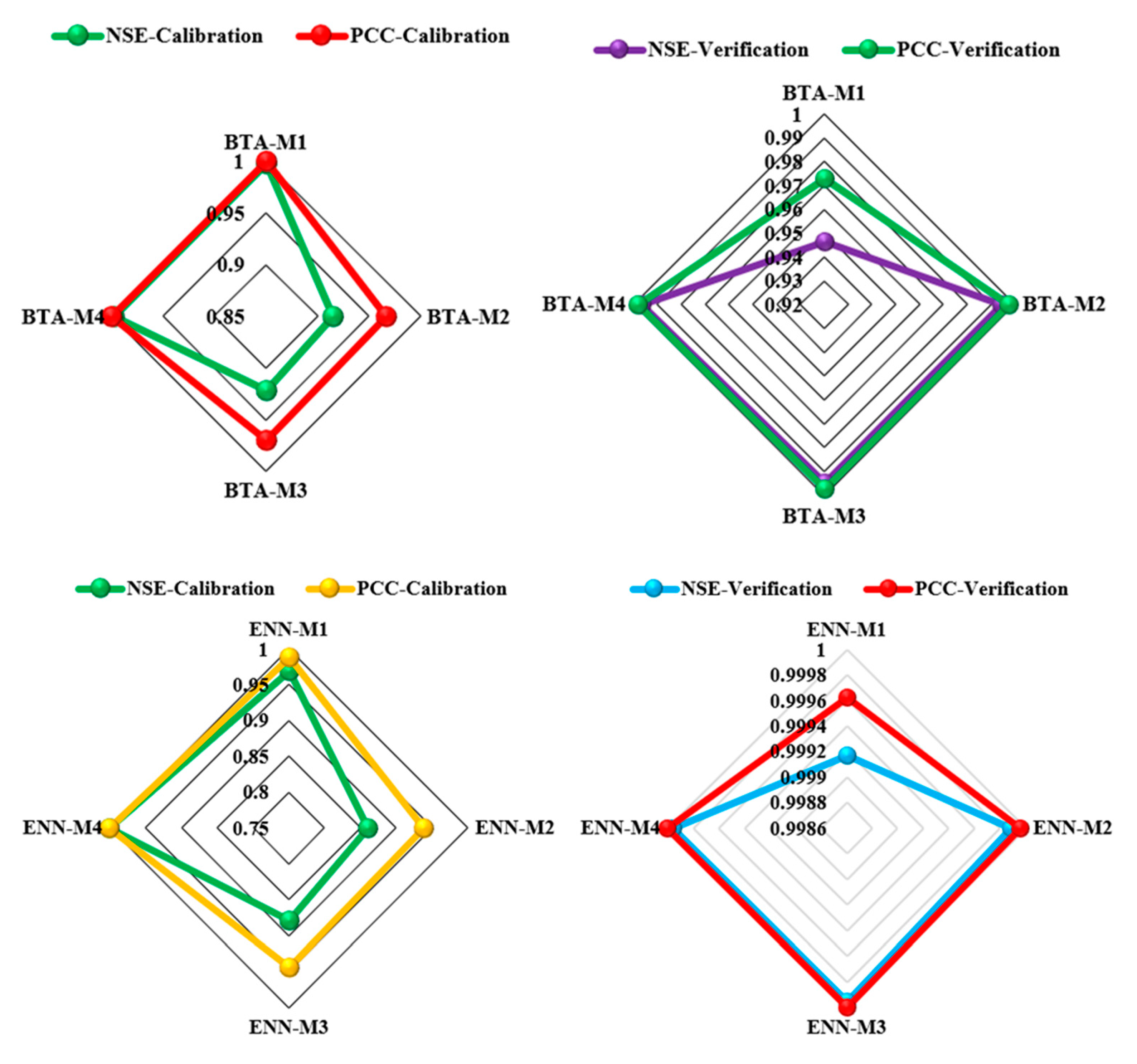
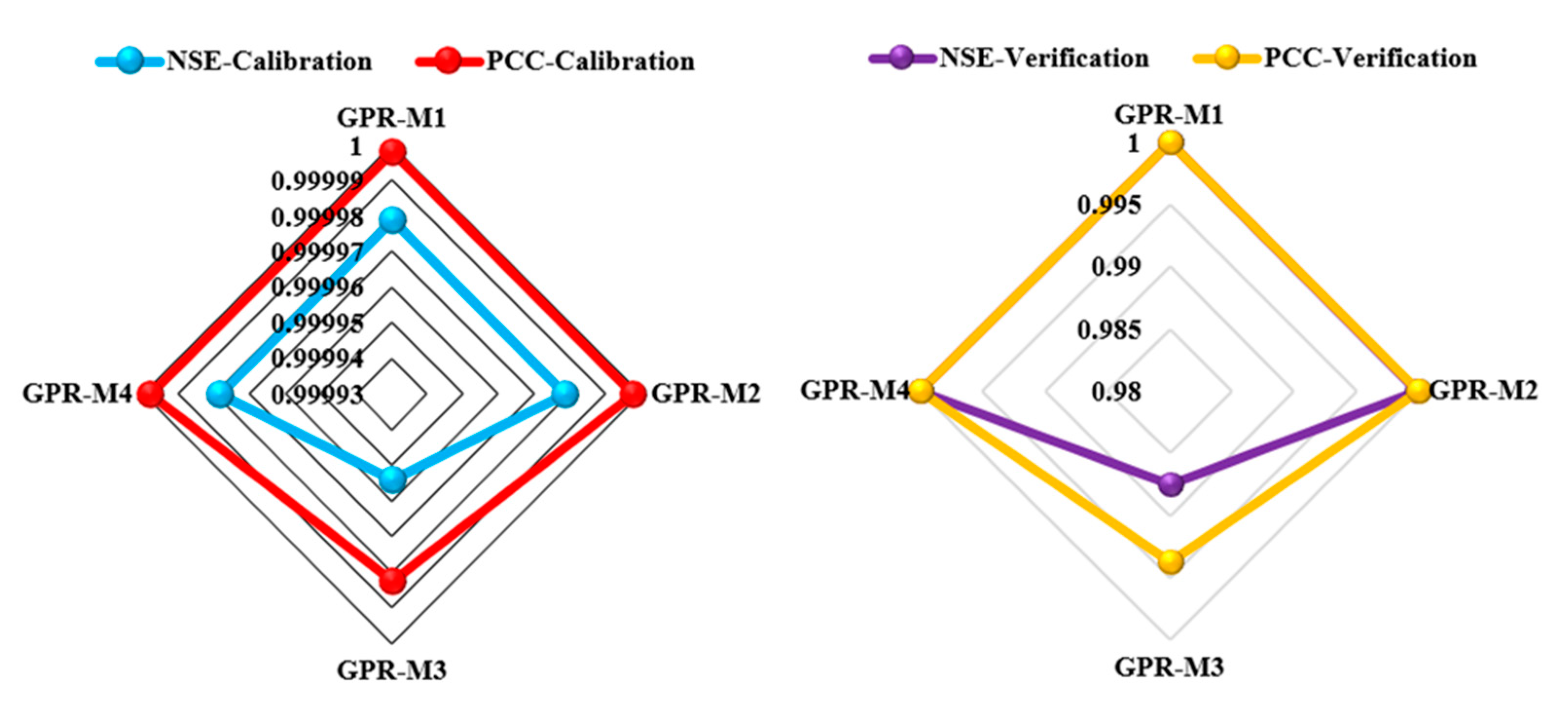
This section analyses the second scenario II based on inverter modelling ACP (kW) using several soft computing approaches. Going at the results in Table 3, BTA-M1, BTA-M2, BTA-M3, BTA-M4, GPR-M1, GPR-M2, GPR-M3, and GPR-M4 models have high NSE values (above 0.9), indicating that they perform well in capturing the variation in the data. On the other hand, ENN-M1, ENN-M2, and ENN-M3 models have lower NSE values, indicating that they do not capture the data variation as well as the other models. The PCC values for most of the models are high (above 0.9), indicating that they have a strong linear relationship with the observed data. However, the ENN-M2 model has a relatively low PCC value of 0.939, indicating that its relationship with the observed data is not as strong as the other models (see Figure 6). Similarly, the RMSE values for most of the models are relatively low, indicating that the models have low prediction errors.
However, the ENN-M2 model has a higher RMSE value of 0.094, indicating that it has higher prediction errors than the other models. The MAPE values for the BTA-M1, BTA-M2, and BTA-M3 models are high (above 30%), indicating that they have relatively high prediction errors. The ENN-M1 and ENN-M2 models also have high MAPE values (above 40%). The MAE values for most of the models are relatively low, indicating that they have low absolute prediction errors. However, the ENN-M1 and ENN-M2 models have higher MAE values than the other models. The PBIAS values for most of the models are close to zero, indicating that they have no significant bias in their predictions. However, the ENN-M1 and ENN-M2 models have negative PBIAS values, indicating that they tend to underpredict the observed data. Generally, the BTA-M1, BTA-M2, BTA-M3, BTA-M4, GPR-M1, GPR-M2, GPR-M3, and GPR-M4 models perform well in the calibration phase, while the ENN-M1, ENN-M2, and ENN-M3 models have relatively lower performance measures. This results is in line with one reported by [51] to predict PV panel behaviors under realistic weather conditions. R2, MSE, and MAPE values for the optimal ANN model of the proposed method were 0.971, 0.002 and 0.107, respectively. A comparative study among ANN and analytical models was also carried out. Among the analytical models, the five-parameter model, with MAPE = 0.112, MSE = 0.0026 and R2 = 0.919, gave better prediction than the four-parameter model (with MAPE = 0.152, MSE = 0.0052 and R2 = 0.905).
Similarly, the table provides a quick way to compare and evaluate the performance of different models in verification phase, but it is important to consider the context and purpose of the models before drawing conclusions based solely on the metrics presented. The numerical comparison of the models based on these metrics indicated that NSE: The models with the highest NSE are ENN-M2, ENN-M3, ENN-M4, GPR-M1, GPR-M2, and GPR-M4, all with a perfect score of 1. The model with the lowest NSE is GPR-M3 with a score of 0.988. While the models with the highest PCC are ENN-M2, ENN-M3, ENN-M4, GPR-M1, GPR-M2, and GPR-M4, all with a perfect score of 1. The model with the lowest PCC is BTA-M1 with a score of 0.973. The model with the lowest RMSE is BTA-M4 with a score of 0.02. The model with the highest RMSE is GPR-M3 with a score of 68.185. According to [52,53,54], MAPE values is good when it is below or equal to 10%. MAPE: The model with the lowest MAPE is ENN-M4 with a score of 0.506%. The model with the highest MAPE is BTA-M1 with a score of 10.091%. Similarly, the model with the lowest MAE is BTA-M4 with a score of 0.013. The model with the highest MAE is BTA-M1 with a score of 0.095. To compare the accuracy again with recent literature, [55] reported the use of ML to process big data by monitoring the behavior of PV. The monitoring system was reported to have the capability of detecting PV system failure with an RMSE of 0.66. The accuracy of the proposed model with respect to real-time data for clear days has an RMSE error of 73.71 and an R-squared is calculated at 0.95. This accuracy is also in line with the current study outcomes.
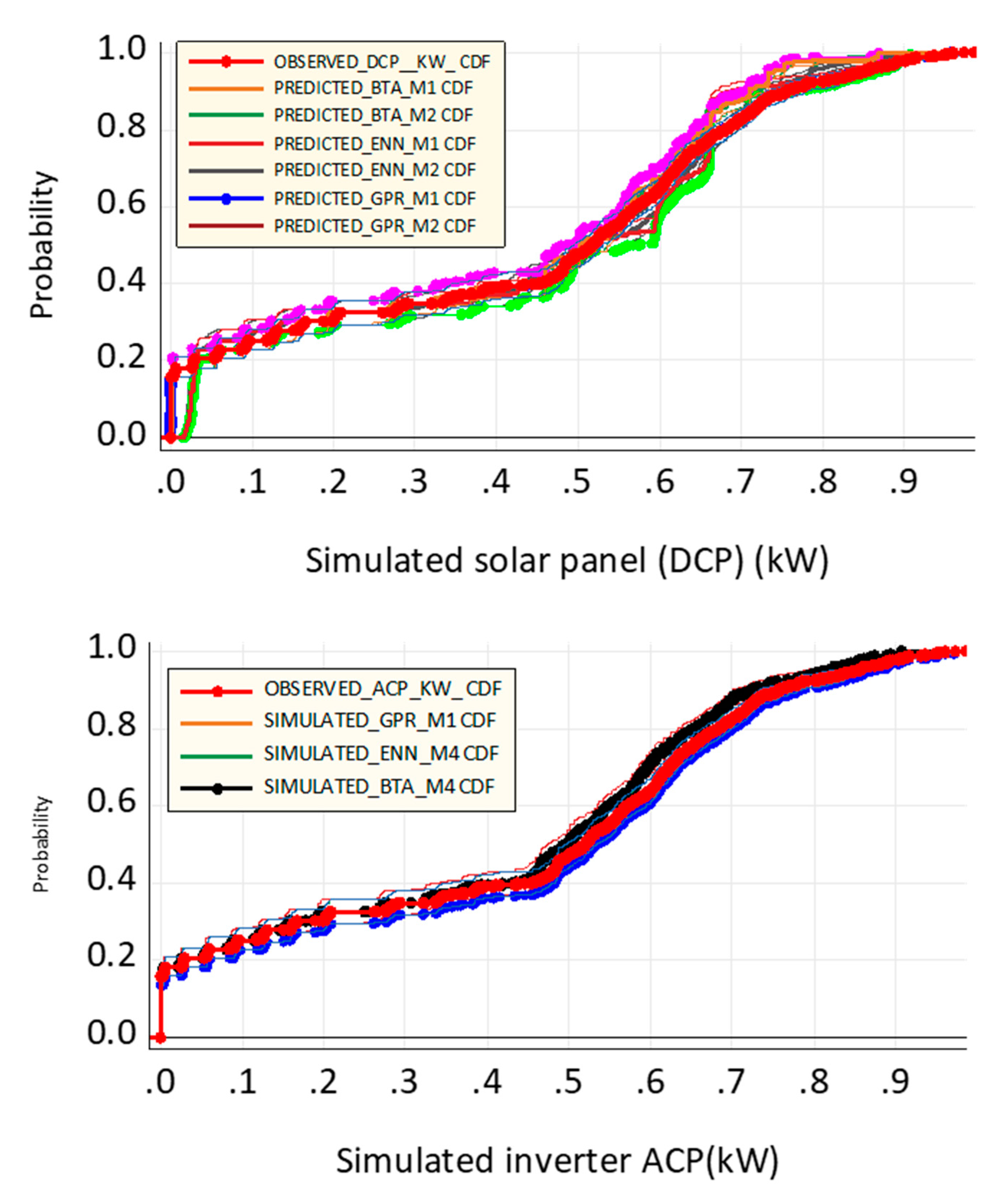
The numerical comparison was also discussed using PBAIS both in training and testing phase. PBIAS: The models with the lowest PBIAS are GPR-M1 and GPR-M4 with a score of -2.542 and -23.542, respectively. The model with the highest PBIAS is BTA-M2 with a score of 801.107. Based on these metrics, ENN-M4 appears to be the best performing model, with perfect scores in NSE, PCC, and relatively low scores in RMSE, MAPE, MAE, and PBIAS. BTA-M1, on the other hand, has relatively high scores in RMSE, MAPE, MAE, and PBIAS, indicating lower performance than other models. It is important to note that these metrics alone may not be sufficient to determine the best model for a specific task, and other factors such as computational efficiency and interpretability should also be considered [56,57,58]. Similarly, [6] presents an intelligent photovoltaic (PV) fault detection system using Adaptive Neuro-Fuzzy Inference System (ANFIS) methodology. To accomplish this objective, it is necessary to train the ANFIS model for an effective PV fault detection and classification system by deploying Grid Partition (GP) and Subtractive Clustering (SC) strategies using some research data. The values obtained from statistical analysis such as coefficient correlation R, root mean squared error (RMSE), and coefficient of determination R2 were 0.9989, 0.0383, and 0.9978. These obtained results show that the ANFIS SC framework with cluster radius 0.6 can remarkably diagnose the PV system faults with high accuracy. The overall accuracy of both the scenarios can be presented in Figure 7, using the probability distribution function graph.

5. Conclusions

In conclusion, this paper proposes a novel approach to fault detection and diagnosis in PV arrays and inverters using a combination of AI techniques, including Elman Neural Network, Boosted Tree Algorithms, Multi-layer Perceptron, and Gaussian Processes Regression. The proposed approach integrates the strengths of each algorithm for enhanced accuracy and reliability in fault diagnosis, with ENN utilized for feature extraction, and BTA, MLP, and GPR integrated for fault detection and diagnosis. Two intelligent learning scenarios are carried out, one for the PV array fault detection with DC power as output and the other for inverter fault detection with AC power as output. The proposed technique demonstrates superior accuracy and reliability compared to existing fault detection techniques. It is capable of detecting various types of faults in PV arrays and inverters, providing a reliable solution for enhancing the performance and reliability of solar energy systems.
The results of the evaluation on a real-world solar energy dataset demonstrate that the proposed approach outperforms existing fault detection techniques, achieving higher accuracy and better performance. Moreover, the proposed technique can be extended to other renewable energy systems, providing a basis for developing comprehensive fault detection and diagnosis frameworks. This research represents a significant contribution to the field of solar energy systems and fault detection and diagnosis. The proposed technique offers a promising solution for increasing the reliability and efficiency of renewable energy systems, which are becoming increasingly important as the demand for clean energy continues to grow. The proposed approach can help to reduce the cost of maintenance and increase the lifespan of solar energy systems, leading to more efficient and sustainable use of renewable energy resources. The research opens the door for further advancements in the field of fault detection and diagnosis in solar energy systems, with the potential for significant impact in the development of more efficient and reliable renewable energy systems.

Author Contributions

“Conceptualization, A.A, C.F.M.A, M.G and S.I.A.; methodology, A.A, and M.M.J; software, M.M.J; validation, C.F.M.A, M.G and S.I.A.; formal analysis, A.A and M.N.Y; investigation, A.A.; resources, C.F.M.A and M.G; data curation, M.M.J; writing—original draft preparation, A.A.; writing—review and editing, S.I.A.; visualization, M.M.J; supervision, C.F.M.A; project administration, M.G; funding acquisition, A.A. All authors have read and agreed to the published version of the manuscript.”

Funding

This research was partly funded by Coordenação de Aperfeiçoamento de Pessoal de Nível Superior (CAPES) (No. 88887.514132/2020-00).

Institutional Review Board Statement

Not applicable.

Informed Consent Statement

Not applicable.

Data Availability Statement

Not applicable.

Acknowledgments

The authors kindly thank ENERQ-CTPEA Centro de Estudos em Regulação Qualidade de Energia for their support.

Conflicts of Interest

The authors declare no conflict of interest.

References

  1. A. Abubakar, C. F. M. Almeida, and M. Gemignani, “Review of Artificial Intelligence-Based Failure Detection and Diagnosis Methods for Solar Photovoltaic Systems,” Machines, vol. 9, no. 12, p. 328, Dec. 2021. [CrossRef]
  2. D. Feldman, K. Dummit, J. Zuboy, J. Heeter, K. Xu, and R. Margolis, “Spring 2022 Solar Industry Update,” 2022.
  3. D. Feldman, K. Dummit, J. Zuboy, and R. Margolis, “Winter 2023 Solar Industry Update,” 2023.
  4. Y. Zhao, R. Ball, J. Mosesian, J. de Palma, and B. Lehman, “Graph-Based Semi-supervised Learning for Fault Detection and Classification in Solar Photovoltaic Arrays,” IEEE Trans. Power Electron., vol. 30, no. 5, pp. 2848–2858, 2015. [CrossRef]
  5. B. Taghezouit, F. Harrou, Y. Sun, A. H. Arab, and C. Larbes, “A simple and effective detection strategy using double exponential scheme for photovoltaic systems monitoring,” Sol. Energy, vol. 214, no. December 2020, pp. 337–354, 2021. 20 December. [CrossRef]
  6. M. Abbas and D. Zhang, “A smart fault detection approach for PV modules using Adaptive Neuro-Fuzzy Inference framework,” Energy Reports, vol. 7, pp. 2962–2975, 2021. [CrossRef]
  7. D. Korkmaz and H. Acikgoz, “An efficient fault classification method in solar photovoltaic modules using transfer learning and multi-scale convolutional neural network,” Eng. Appl. Artif. Intell., vol. 113, no. April, p. 104959, 2022. [CrossRef]
  8. A. Mellit, “An embedded solution for fault detection and diagnosis of photovoltaic modules using thermographic images and deep convolutional neural networks,” Eng. Appl. Artif. Intell., vol. 116, no. June, p. 105459, 2022. [CrossRef]
  9. D. Manno, G. Cipriani, G. Ciulla, V. Di Dio, S. Guarino, and V. Lo Brano, “Deep learning strategies for automatic fault diagnosis in photovoltaic systems by thermographic images,” Energy Convers. Manag., vol. 241, no. May, p. 114315, 2021. [CrossRef]
  10. A. Mellit and S. Kalogirou, “Artificial intelligence and internet of things to improve efficacy of diagnosis and remote sensing of solar photovoltaic systems: Challenges, recommendations and future directions,” Renewable and Sustainable Energy Reviews, vol. 143, no. January. Elsevier Ltd, p. 110889, 2021. [CrossRef]
  11. A. G. Olabi et al., “Artificial neural networks applications in partially shaded PV systems,” Thermal Science and Engineering Progress, vol. 37, no. May 2022. Elsevier Ltd, p. 101612, 2023. [CrossRef]
  12. A. Mellit and S. Kalogirou, “Assessment of machine learning and ensemble methods for fault diagnosis of photovoltaic systems,” Renew. Energy, vol. 184, pp. 1074–1090, 2022. [CrossRef]
  13. L. Hocine, K. M. Samira, M. Tarek, N. Salah, and K. Samia, “Automatic detection of faults in a photovoltaic power plant based on the observation of degradation indicators,” Renew. Energy, vol. 164, pp. 603–617, 2021. [CrossRef]
  14. S. Naveen Venkatesh, B. Rebecca Jeyavadhanam, A. M. Moradi Sizkouhi, S. M. Esmailifar, M. Aghaei, and V. Sugumaran, “Automatic detection of visual faults on photovoltaic modules using deep ensemble learning network,” Energy Reports, vol. 8, pp. 14382–14395, 2022. [CrossRef]
  15. S. Sarikh, M. Raoufi, A. Bennouna, and B. Ikken, “Characteristic curve diagnosis based on fuzzy classification for a reliable photovoltaic fault monitoring,” Sustain. Energy Technol. Assessments, vol. 43, no. November 2020, p. 100958, 2021. [CrossRef]
  16. A. Seghiour, H. A. Abbas, A. Chouder, and A. Rabhi, “Deep learning method based on autoencoder neural network applied to faults detection and diagnosis of photovoltaic system,” Simul. Model. Pract. Theory, vol. 123, no. September 2021, p. 102704, 2023. [CrossRef]
  17. S. Jadidi, H. Badihi, and Y. Zhang, “Design of an intelligent hybrid diagnosis scheme for cyber-physical PV systems at the microgrid level,” Int. J. Electr. Power Energy Syst., vol. 150, no. October 2022, p. 109062, 2023. [CrossRef]
  18. X. Lu et al., “Efficient fault diagnosis approach for solar photovoltaic array using a convolutional neural network in combination of generative adversarial network under small dataset,” Sol. Energy, vol. 253, no. February 2022, pp. 360–374, 2023. [CrossRef]
  19. D. O. Tojeiro, R. T. Cabeza, and A. S. Potts, “Fault detection based on Neuro-Fuzzy models and residual evaluation with fuzzy thresholds applied to a photovoltaic system,” in IFAC-PapersOnLine, 2021, vol. 54, no. 20, pp. 717–722. [CrossRef]
  20. Y. Liu et al., “Fault diagnosis approach for photovoltaic array based on the stacked auto-encoder and clustering with I-V curves,” Energy Convers. Manag., vol. 245, p. 114603, 2021. [CrossRef]
  21. N. Kellil, A. Aissat, and A. Mellit, “Fault diagnosis of photovoltaic modules using deep neural networks and infrared images under Algerian climatic conditions,” Energy, vol. 263, no. PC, p. 125902, 2023. [CrossRef]
  22. V. Nourani, G. Elkiran, and S. I. Abba, “Wastewater treatment plant performance analysis using artificial intelligence – an ensemble approach,” Water Sci. Technol., 2018. [CrossRef]
  23. L. Q. Shen, G. Amatulli, T. Sethi, P. Raymond, and S. Domisch, “Estimating nitrogen and phosphorus concentrations in streams and rivers, within a machine learning framework,” Sci. Data, vol. 7, no. 1, pp. 1–12, 2020. [CrossRef]
  24. M. Wang, L. Ma, M. Strokal, W. Ma, X. Liu, and C. Kroeze, “Hotspots for Nitrogen and Phosphorus Losses from Food Production in China: A County-Scale Analysis,” Environ. Sci. Technol., vol. 52, no. 10, pp. 5782–5791, 2018. [CrossRef]
  25. J. Zhou, Y. Zhang, K. Wu, M. Hu, H. Wu, and D. Chen, “National estimates of environmental thresholds for upland soil phosphorus in China based on a meta-analysis,” Sci. Total Environ., vol. 780, p. 146677, 2021. [CrossRef]
  26. Y. Zhang et al., “Estimation of nitrogen runoff loss from croplands in the Yangtze River Basin: A meta-analysis,” Environ. Pollut., vol. 272, no. xxxx, p. 116001, 2021. [CrossRef]
  27. G. Elkiran, V. Nourani, and S. I. Abba, “Multi-step ahead modelling of river water quality parameters using ensemble artificial intelligence-based approach,” J. Hydrol., vol. 577, no. July, p. 123962, 2019. [CrossRef]
  28. G. R. Rakhshandehroo, M. Vaghefi, and M. A. Aghbolaghi, “Forecasting Groundwater Level in Shiraz Plain Using Artificial Neural Networks,” Arab. J. Sci. Eng., vol. 37, no. 7, pp. 1871–1883, 2012. [CrossRef]
  29. P. Di et al., “Ultra-Short Term Load Forecasting Based on Elman Neural Network,” 2019 IEEE PES Innov. Smart Grid Technol. Asia, ISGT 2019, vol. 2, pp. 911–915, 2019. [CrossRef]
  30. H. Jia and B. Taheri, “Model identification of Solid Oxide Fuel Cell using hybrid Elman Neural Network/Quantum Pathfinder algorithm,” Energy Reports, vol. 7, pp. 3328–3337, 2021. [CrossRef]
  31. J. Wang, W. Zhang, Y. Li, J. Wang, and Z. Dang, “Forecasting wind speed using empirical mode decomposition and Elman neural network,” Appl. Soft Comput. J., vol. 23, pp. 452–459, 2014. [CrossRef]
  32. A. O. Alnahit, A. K. Mishra, and A. A. Khan, “Stream water quality prediction using boosted regression tree and random forest models,” Stoch. Environ. Res. Risk Assess., vol. 4, 2022. [CrossRef]
  33. J. Elith, J. R. Leathwick, and T. Hastie, “A working guide to boosted regression trees,” J. Anim. Ecol., vol. 77, no. 4, pp. 802–813, 2008. [CrossRef]
  34. I.K. Umar, V. Nourani, H. Gökçekuş, and S. I. Abba, “An intelligent hybridized computing techniques for the prediction of roadway traffic noise based on non-linear mutual information,” vol. 5, 2022. [CrossRef]
  35. A. Mosavi, P. Ozturk, and K. W. Chau, “Flood prediction using machine learning models: Literature review,” Water (Switzerland), vol. 10, no. 11, pp. 1–40, 2018. [CrossRef]
  36. U. Stańczyk, B. Zielosko, and L. C. Jain, Advances in feature selection for data and pattern recognition: An introduction, vol. 138. 2018.
  37. W. S. Kemal and M. Alhasa, SPRINGER BRIEFS IN METEOROLOGY Modeling of Tropospheric Delays Using ANFIS. 2016.
  38. A. Elbeltagi et al., “Applications of Gaussian process regression for predicting blue water footprint: Case study in Ad Daqahliyah, Egypt,” Agric. Water Manag., vol. 255, 2021. [CrossRef]
  39. K. Kargar et al., “Estimating longitudinal dispersion coefficient in natural streams using empirical models and machine learning algorithms,” Eng. Appl. Comput. Fluid Mech., vol. 14, no. 1, pp. 311–322, 2020. [CrossRef]
  40. E. Momeni, M. B. Dowlatshahi, F. Omidinasab, H. Maizir, and D. J. Armaghani, “Gaussian Process Regression Technique to Estimate the Pile Bearing Capacity,” Arab. J. Sci. Eng., vol. 45, no. 10, pp. 8255–8267, 2020. [CrossRef]
  41. C. Huang, Z. Zhao, L. Wang, Z. Zhang, and X. Luo, “Point and interval forecasting of solar irradiance with an active Gaussian process,” IET Renew. Power Gener., vol. 14, no. 6, pp. 1020–1030, 2020. [CrossRef]
  42. A.G. Usman, S. IŞIK, and S. I. Abba, “Qualitative prediction of Thymoquinone in the high-performance liquid chromatography optimization method development using artificial intelligence models coupled with ensemble machine learning,” Sep. Sci. Plus, no. June, pp. 1–9, 2022. [CrossRef]
  43. S. I. Abba, G. Elkiran, and V. Nourani, “Improving novel extreme learning machine using pca algorithms for multi-parametric modeling of the municipal wastewater treatment plant,” Desalin. Water Treat., vol. 215, no. March, pp. 414–426, 2021. [CrossRef]
  44. K. Bala, I. Etikan, and A. G. Usman, “Artificial-Intelligence-Based Models Coupled with Correspondence Analysis Visualization on ART — Cases from Gombe State , Nigeria : A Comparative Study,” 2023.
  45. M. Saood et al., “New generation neurocomputing learning coupled with a hybrid neuro-fuzzy model for quantifying water quality index variable : A case study from Saudi Arabia,” Ecol. Inform., vol. 70, no. May, p. 101696, 2022. [CrossRef]
  46. A. Alamrouni, F. Aslanova, S. Mati, H. S. Maccido, and A. A. Jibril, “Multi-Regional Modeling of Cumulative COVID-19 Cases Integrated with Environmental Forest Knowledge Estimation : A Deep Learning Ensemble Approach,” Int. J. Environ. Res. Public Heal., vol. 19(2), pp. 1–23, 2022. [CrossRef]
  47. A. G. Usman, M. H. Ahmad, N. Danraka, and S. I. Abba, “The effect of ethanolic leaves extract of Hymenodictyon floribundun on inflammatory biomarkers : A data - driven approach,” Bull. Natl. Res. Cent., 2021. [CrossRef]
  48. M. Dhimish, V. Holmes, B. Mehrdadi, and M. Dales, “Diagnostic method for photovoltaic systems based on six layer detection algorithm,” Electr. Power Syst. Res., vol. 151, pp. 26–39, 2017. [CrossRef]
  49. D. Adhya, S. Chatterjee, and A. K. Chakraborty, “Performance assessment of selective machine learning techniques for improved PV array fault diagnosis,” Sustain. Energy, Grids Networks, vol. 29, p. 100582, 2022. [CrossRef]
  50. S. L. P, S. S, and M. S. Rayudu, “IoT based solar panel fault and maintenance detection using decision tree with light gradient boosting,” Meas. Sensors, vol. 27, no. November 2022, p. 100726, 2023. [CrossRef]
  51. M. Karamirad, M. Omid, R. Alimardani, H. Mousazadeh, and S. N. Heidari, “ANN based simulation and experimental verification of analytical four- and five-parameters models of PV modules,” Simul. Model. Pract. Theory, vol. 34, pp. 86–98, 201. [CrossRef]
  52. M. S. Gaya et al., “Estimation of water quality index using artificial intelligence approaches and multi-linear regression,” vol. 9, no. 1, pp. 126–134, 2020. [CrossRef]
  53. S. I. Abba et al., “Modelling of Uncertain System: A comparison study of Linear and Non-Linear Approaches,” 2019 IEEE Int. Conf. Autom. Control Intell. Syst. I2CACIS 2019 - Proc., no. October, pp. 1–6, 2019. [CrossRef]
  54. M. S. Gaya, N. A. Wahab, Y. Sam, and S. I. Samsuddin, “Comparison of ANFIS and Neural Network Direct Inverse Control Applied to Wastewater Treatment System,” vol. 845, pp. 543–548, 2014. [CrossRef]
  55. Arévalo, D. Benavides, M. Tostado-Véliz, J. A. Aguado, and F. Jurado, “Smart monitoring method for photovoltaic systems and failure control based on power smoothing techniques,” Renew. Energy, vol. 205, no. October 2022, pp. 366–383, 2023. 20 October. [CrossRef]
  56. H. Adamu, I. Abba, and B. Anyin, “Energy Advances of high-performance electrochemical energy storage systems through feature engineering of multiple descriptor families of materials,” 2023. [CrossRef]
  57. Abdullahi, G. Elkiran, S. I. Malami, A. Rotimi, S. I. Haruna, and S. I. Abba, “Compatibility of Hybrid Neuro-Fuzzy Model to Predict Reference Evapotranspiration in Distinct Climate Stations,” pp. 1–6, 2022. [CrossRef]
  58. S. I. Malami, F. H. Anwar, S. Abdulrahman, S. I. Haruna, S. I. A. Ali, and S. I. Abba, “Implementation of hybrid neuro-fuzzy and self-turning predictive model for the prediction of concrete carbonation depth: A soft computing technique,” Results Eng., vol. 10, no. May, p. 100228, 2021. [CrossRef]
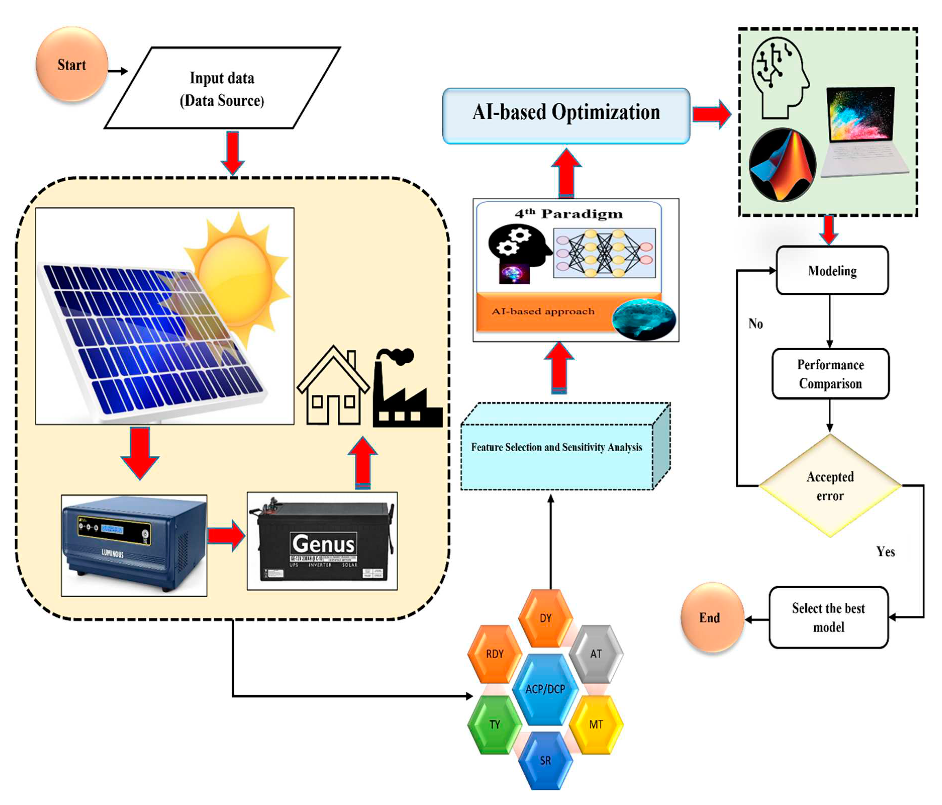
Figure 1. Proposed modelling scheme.
Preprints 80376 g001
Figure 3. Raw data for input-output variables.
Preprints 80376 g003
Figure 4. Raw data for input-output variables.
Preprints 80376 g004
Figure 5. Embedded scatter plot in the verification phase.
Preprints 80376 g005
Figure 6. Radar plot showing the goodness-of-fit for modelling ACP inverter.
Preprints 80376 g006aPreprints 80376 g006b
Figure 7. Probability distribution function graph for DCP and ACP simulated approach.
Preprints 80376 g007
Table 1. Descriptive statistic for input-output variables.
Parameters Mean SD Kurtosis Skewness Minimum Maximum
DY 2401.47 2667.09 -1.20 0.64 0.00 7190.00
TY 7620392.92 451795.89 -1.05 -0.45 6870716.67 8460553.49
AT 28.42 3.75 -0.54 0.67 22.67 39.17
MT 34.65 13.71 -0.65 0.85 20.16 72.83
SR 0.26 0.34 -0.21 1.05 0.00 1.36
DCP 3775.04 4045.64 -1.20 0.52 0.00 13687.94
ACP 369.50 395.76 -1.21 0.52 0.00 1334.94
Table 2. The predicted results for solar panel modelling.
Calibration Phase
NSE PCC RMSE MAPE MAE PBIAS
BTA-M1 0.914 0.967 0.072 35.267 0.043 0.044
BTA-M2 0.921 0.970 0.070 33.745 0.041 0.044
ENN-M1 0.973 0.990 0.045 22.100 0.019 -58.588
ENN-M2 0.971 0.989 0.047 22.528 0.021 -69.997
GPR-M1 1.000 1.000 0.000 29.597 0.000 0.000
GPR-M2 1.000 1.000 0.002 29.711 0.001 0.000
Verification Phase
NSE PCC RMSE MAPE MAE PBIAS
BTA-M1 0.969 0.989 0.049 6.876 0.031 17460.222
BTA-M2 0.969 0.989 0.048 6.866 0.031 17140.021
ENN-M1 0.968 0.985 0.051 22.150 0.039 -58.638
ENN-M2 0.966 0.984 0.053 22.578 0.041 -70.047
GPR-M1 1.000 1.000 0.000 0.083 0.000 0.000
GPR-M2 1.000 1.000 0.000 0.091 0.000 0.000
Table 3. The predicted results for inverter modelling.
Calibration Phase
NSE PCC RMSE MAPE MAE PBIAS
BTA-M1 0.997 1.000 0.014 27.247 0.008 0.040
BTA-M2 0.915 0.966 0.073 35.294 0.043 0.040
BTA-M3 0.921 0.969 0.070 34.136 0.041 0.040
BTA-M4 0.997 1.000 0.014 27.247 0.008 0.040
ENN-M1 0.970 0.988 0.046 43.989 0.043 -0.066
ENN-M2 0.860 0.939 0.094 43.518 0.063 -0.021
ENN-M3 0.880 0.945 0.090 36.625 0.059 -0.012
ENN-M4 1.000 1.000 0.001 28.886 0.001 -0.004
GPR-M1 1.000 1.000 0.001 29.721 0.001 -0.004
GPR-M2 1.000 1.000 0.001 29.731 0.001 -0.004
GPR-M3 1.000 1.000 0.002 29.820 0.001 -0.004
GPR-M4 1.000 1.000 0.001 29.733 0.001 -0.004
Verification Phase
NSE PCC RMSE MAPE MAE PBIAS
BTA-M1 0.947 0.973 0.061 10.091 0.095 101.107
BTA-M2 0.995 0.997 0.088 6.069 0.018 801.107
BTA-M3 0.995 0.997 0.088 5.085 0.017 60.107
BTA-M4 0.997 0.998 0.020 4.291 0.013 30.107
ENN-M1 0.999 1.000 0.008 6.424 0.006 -57.560
ENN-M2 1.000 1.000 0.003 1.397 0.003 -49.126
ENN-M3 1.000 1.000 0.002 1.205 0.002 -42.401
ENN-M4 1.000 1.000 0.002 0.506 0.002 -42.302
GPR-M1 1.000 1.000 0.002 0.363 0.002 -2.542
GPR-M2 1.000 1.000 0.003 1.006 0.002 -173.542
GPR-M3 0.988 0.994 68.185 1.006 2.281 87.330
GPR-M4 1.000 1.000 0.002 0.393 0.002 -23.542
Disclaimer/Publisher’s Note: The statements, opinions and data contained in all publications are solely those of the individual author(s) and contributor(s) and not of MDPI and/or the editor(s). MDPI and/or the editor(s) disclaim responsibility for any injury to people or property resulting from any ideas, methods, instructions or products referred to in the content.
Copyright: This open access article is published under a Creative Commons CC BY 4.0 license, which permit the free download, distribution, and reuse, provided that the author and preprint are cited in any reuse.
Prerpints.org logo

Preprints.org is a free preprint server supported by MDPI in Basel, Switzerland.

Subscribe

© 2024 MDPI (Basel, Switzerland) unless otherwise stated