1. Introduction
According to the most of researchers (Coper et al., 2011, Fielding et al., 2012, Ginkel et al., 2018, Gesusldo, 2019) water insecurity is expected to be intensified in the most parts of the world especially in urban areas. One of the most important threats of urban water security is the population growth and water scarcity. Among the several causes of urban water scarcity, it can be referred to the low rainfall, climate change, high population density, and over allocation of water to the water users. About 27% of the world's population live in areas affected by water scarcity in the mid-2010s. This number will be increased to 42% by 2050 (Boreti and Lorenzo, 2019). Over-urbanization without considering the water resources availability may create a condition of rapidly deteriorating household water security, particularly where pre-existing urban water and sanitation infrastructure is only poorly developed. The two examples of periodic deep-water scarcity that is inducing water insecurity include the California started in early 2000s (Ullrich et al., 2018) and the Cape Town Water Crisis (mid-2017 to mid-2018). In both cases, pre-existing vulnerabilities exacerbated by persistent climatic drought (Muller, 2017). In Australia, water security became a major concern in the late 20th and early 21st century due to population growth (Sue and Lesley, 2020). Water security risks in Bangladesh include a variety of natural climate hazards and the impacts of urbanization as well as those caused from recent climate change like changes in precipitation patterns and sea level rise. The country experiences water security risks for its capital city, Dhaka as well as for its coastal region (Murgatroyd et al., 2021). Many other countries in Middle East such as Libya, Iraq and Syria suffer from water scarcity. Such a crisis has become more problematic due to continued population growth, low precipitation and high water demand for agriculture and industrial uses (Brika, 2019). In Yemen, located in a dry and semi-arid region of the Middle East, severe water crisis is experienced. (Glass, 2010). In Iran, that is located in arid and semi-arid region is currently facing with serious water shortage. The climate change, occurrence of droughts and other social, political and economic problems have aggravated the water crisis. (Khatibi and Arjjumend, 2019). According to Moridi (2017) all development plans in Iran should be take into account the future of population, its growth pattern and prediction of future water needs. Saatsaz (2020) stated that in the modern era, population explosion, industries development, consumerism culture, and unprecedented urbanization coupled with drought events and global warming have brought many difficulties for water sectors. (Mekonnen and Hoekstra, 2016). Furthermore, 30% of population do not have access to safe drinking water (Unicef, 2021). Future water demands in all sectors of cities depend on population growth, economic development, and projected changes in water use efficiency. (Vörösmarty et al., 2000; Liu et al., 2017). Therefore, it is necessary for governments to assess population growth rate and water supply in all regions especially in urban areas (Padowski and Jawitz, 2011; Tolba Abelnga et al., 2022). They concluded that population growth is the most important factor in city water shortages. Mathematical population growth models are commonly used models in prediction of future population (Nizam Uddin et al., 2019). Vinkatasha et al. (2017) described mathematical models for population growth. The two widely used models are the Exponential and Logistic growth models. By these two models, it is possible to study the changes in size of population through time. Andongwisye and Allen (2019) used a mathematical model for predicting Tanzania population growth. They developed the exponential and logistic population growth models in the study. They asserted that the increase in population might lead to expansion of some features that will reduce the carrying capacity of the land and the capability of the common property resources to meet the needs of the present and future populations particularly water and health. Thomas R. Malthus proposed exponential population growth model in 1798. The main assumption in this model is that the increase of population follows a geometric progression. Malthus did not take into account the fact that in any given environment, the growth of population may stop due to the density of population or competition of resources (Aleideh and Alomar, 2019). He assumed that the rate of growth is proportional to the existing population (Cohen, 1995). This logistic model is according to Belgian Mathematician i.e. Verhulst Theory (1840). He showed that the population growth not only depends on the population size but also on how far this size is from its upper limit i.e. its carrying capacity (maximum supportable population). He modified Malthus’s (1798) Model to make the population size proportional to both the previous population and a new term. The word "logistic" has no particular meaning in this context, except that it is commonly accepted. Verhulst Used data from the first five U.S. censuses to predict the U.S. population in 1940 (Lipkin and Smith, 2004). The error of his prediction was less than 1 percent. Literature review indicates that quantitative population estimation are not included in studying of water security of cities. To fill this gap, this study attempts to address it. So that, researchers in different regions before studying water security in a specific region must conduct a study on population dynamic using the historical data. Finally, based on population forecasting information they can make decisions for water consumption and plan for it. In addition, for respond to different water needs in the cities, it is necessary to consider the existing and future condition in terms of water consumption, water demand and water scarcity. The last important point is that the water supply organizations must respond to this question whether the existing infrastructure and accessible water resources will be able to provide their needs or not?
2. Materials and Methods
2.1. Study Area
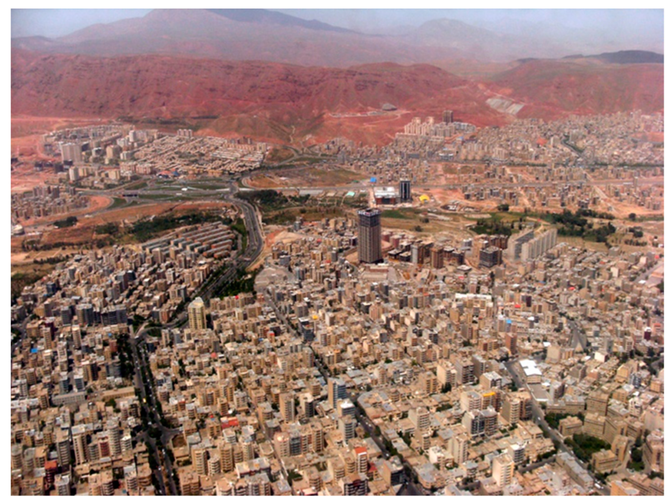
The study area is Tabriz city located in northwestern Iran lies approximately in 38.08 N latitude and 46.29 E longitude. It is the capital of east Azerbaijan province Iran. It is the fifth-most-populous city of Iran. Tabriz’s elevation ranges between 1,350 and 1,600 m (4,430 and 5,250 Ft) above sea level. Tabriz valley opens up into a plain that gently slopes down to the eastern shores of Lake Urmia. Cold winter and temperate dry summer prevailed in this city. Tabriz is the largest economic hub and city area in northwest Iran. Urbanization in the city rapidly developed in recent years. Population of this city, according to the 1956 census was 289996, which increased to 1773033 in 2016 (Iranian Statistics Center, 2022). To respond the population needs, tall buildings were constructed without proper development of urban water infrastructure, especially drinking water (See
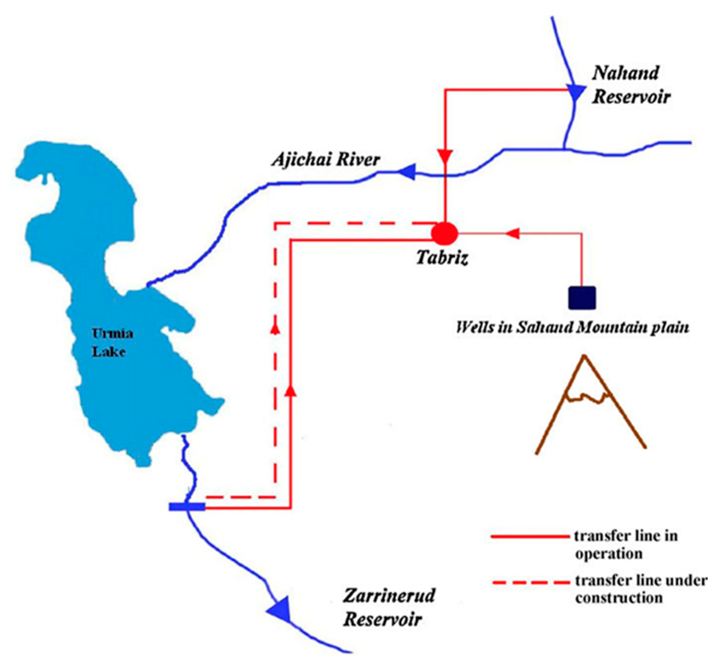
Figure 1). As a result, many habitants use pumps to supply water for high-rise buildings. In addition, Water and Wastewater Company have tried to build several new water reservoirs in different parts of the city. Moreover, portion of drinking water demand provided by transferring water from nearby watershed. Nahand River watershed located in the east of Tabriz city and Zarrineh-Rud river basin located in West Azerbaijan Province are the two watersheds that provide water for Tabriz city (Karimi et al., 2014).
Figure 2 shows the schematic representation of the water transfer to Tabriz. Due to the high consumption rate of urban water, many groundwater wells provide water for city and suburbs. Such a process led to a sharp drop in ground water level.
2.2. Used data
Iranian Statistical Center carried out the census of Iran population regularly in the years 1956, 1966, 1976, 1986, 1996, 2006, 2011 and 2016. These data are readily available for different cities from the official website of the Iranian Statistics Center. In this research, Tabriz population number in deferent years are extracted from the web site (
https://www.amar.org.ir/english/Population-and-Housing-Censuses) and used here. Also, annual water consumption data of Tabriz city obtained from east Azerbaijan's water and wastewater Company from 2011 to 2022 (
https://en.abfaazarbaijan.ir/).
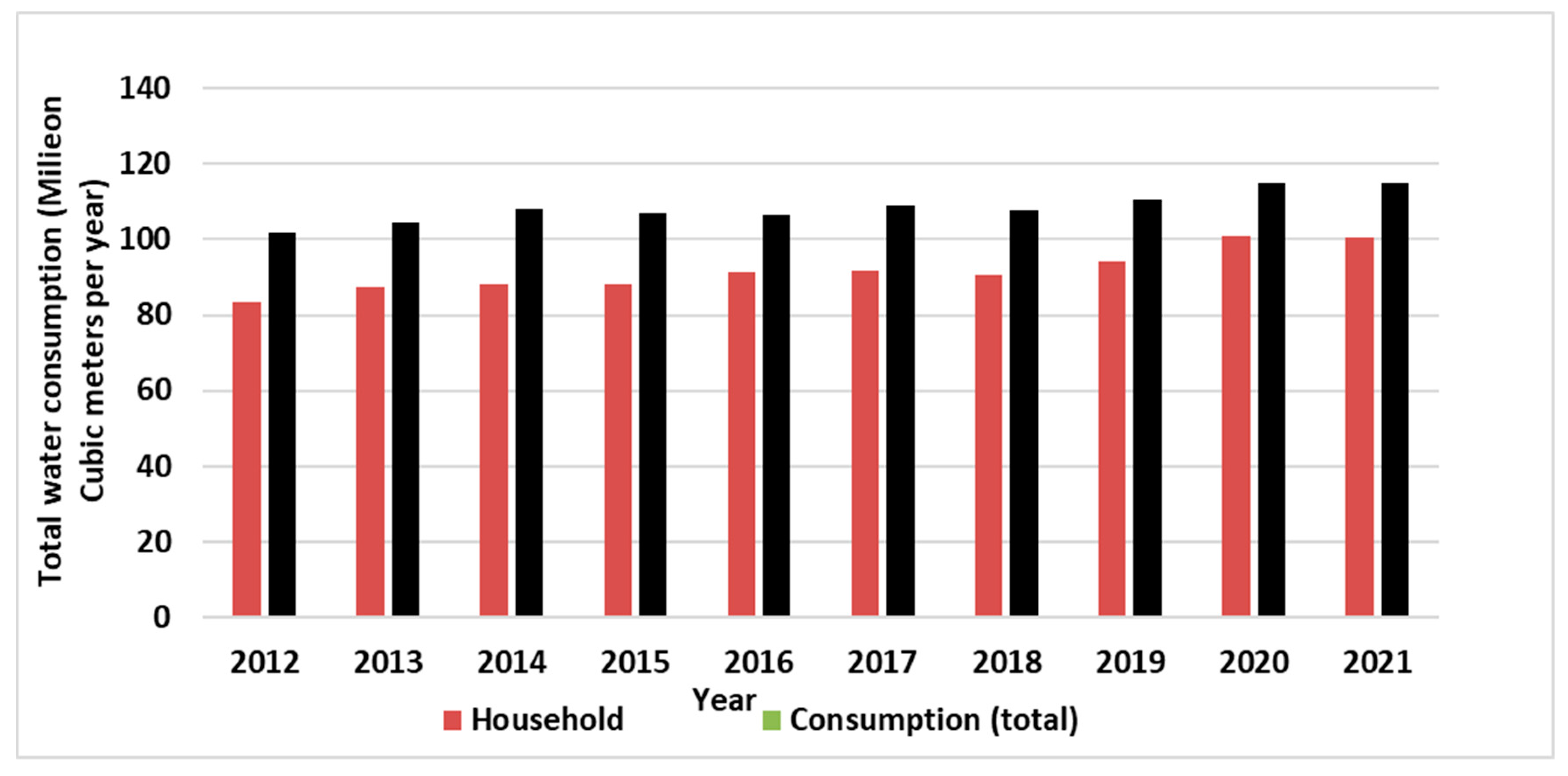
Figure 3a shows the total annual water consumption of Tabriz in the mentioned period. Moreover,
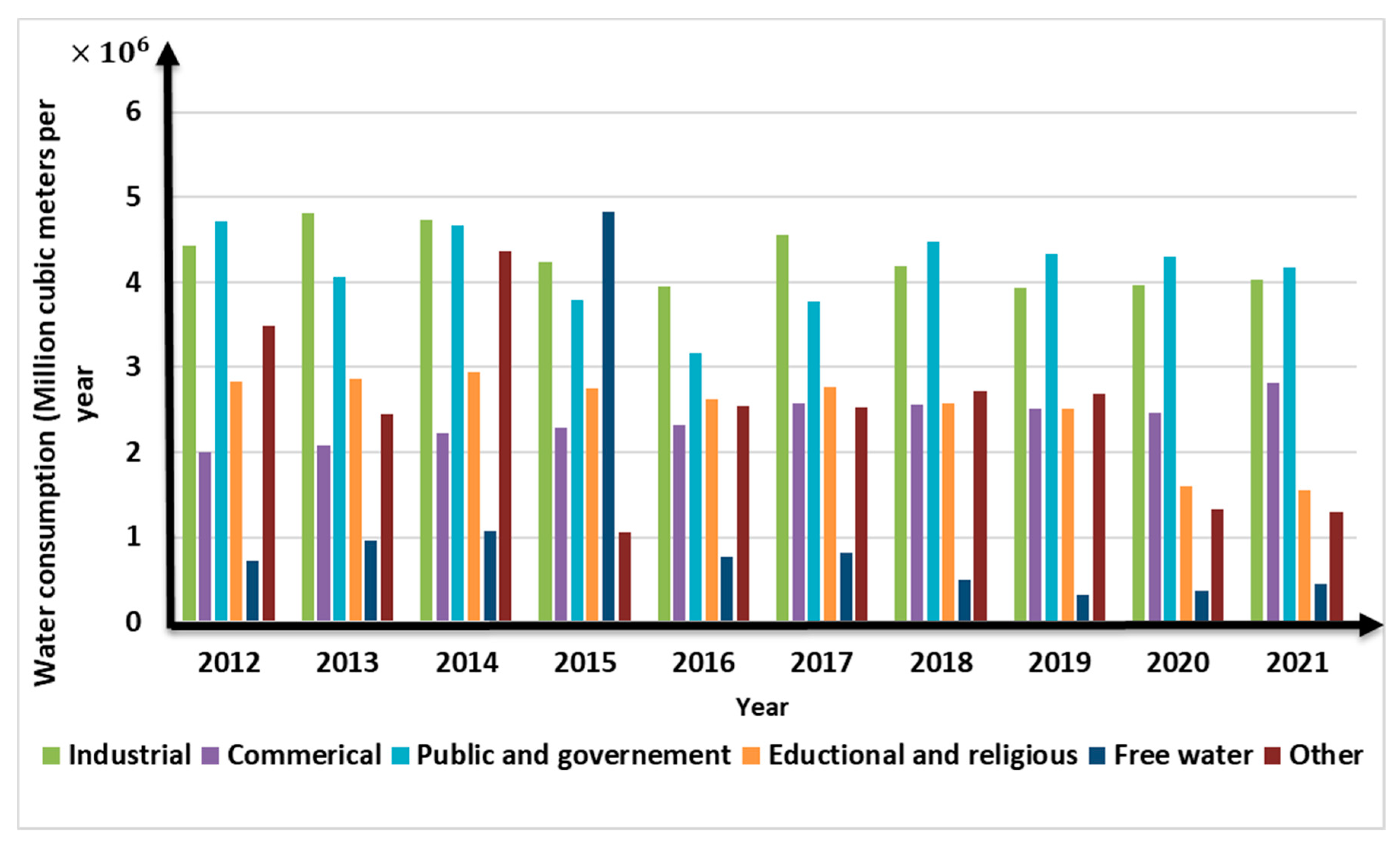
Figure 3b shows the other different sections that used water in Tabriz. As can be seen from it, maximum water consumption belongs to household section. In addition, water consumption increased with growing numbers of people lived in this city.
2.3. Research Framework
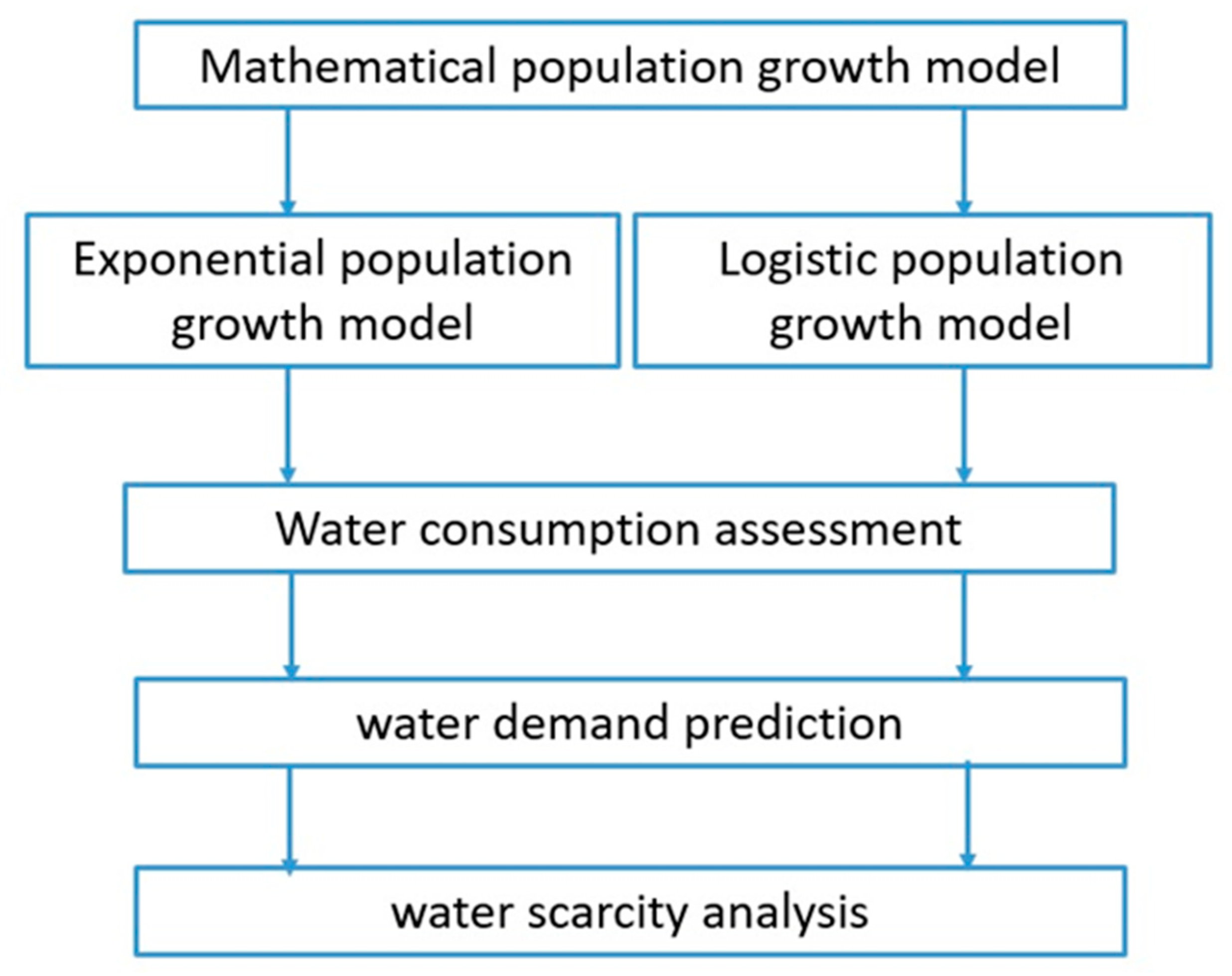
Figure 4 shows a simplified of the present study. As can be seen from
Figure 4 the two mathematical population growth models including i) logistic and ii) exponential were considered. Following derivation of growth models, future people that will be lived in Tabriz was predicted. Correlation analysis were used to find any possible relation between population and water use in Tabriz city. Also, two-regression trend model including linear and quadratic models applied for water demand prediction based on population. To analyze the water scarcity in Tabriz city, three quantitative measures including i) water stress ii) water shortage and iii) per capita water use were used based on population and consumption prediction models.
2.3.1. Population Growth Models
The two used mathematical population growth models were the Logistic and Exponential growth models. The logistic growth model solved symbolically. Then Inflection points and concavity of the logistic growth model were determined for finding maximum corresponding population in Tabriz city. In addition, based on the Logistic and Exponential growth models, the future number of population were calculated between 2022 and 2100. In order to predict water demand in future years, trend analysis conducted to water consumption data series in annual scale using the parametric method of Ordinary Least Square (OLS). Nyamao Nyabwanga et al. (2015) has applied this method in Kisumu city in Kenya. Significance of the slope of trend line tested using the F-Test.
2.3.2. Exponential Population Growth Model
Let the number of individuals at time 𝑡 be denoted by P(t). Malthusian law arises from the solution of the initial value ordinary differential equation.
where P_0>0 denotes the initial population size and k=b-μ, which is the constant per capita growth rate of the population, that is, the average per person number of offspring 𝑏 less the per person average number of deaths 𝜇 (Marsden et al., 2003). The assumption of a constant per capita growth rate leads to the solution of Equation (2).
Which predicts the population growth if k>0, population decrease If k<0, or no changes if k=0. The model may be impractical when the number of generations gets large enough for other factors to come into play (Andongwisye et al., 2019).
2.3.3. Logistic Population Growth Model
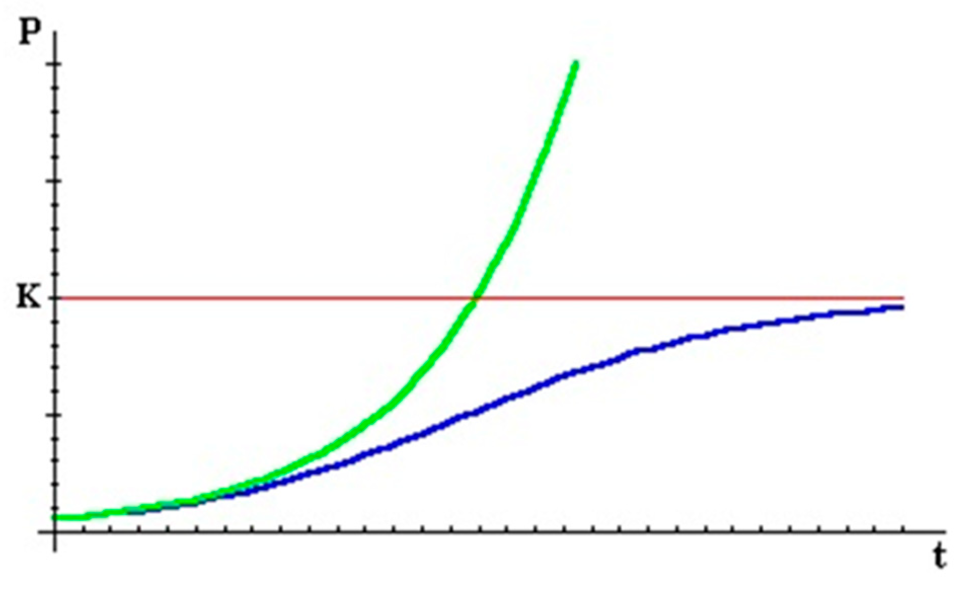
Figure 5 shows two possible curves for growth of a population, the upper curve belongs to the Exponential (unconstrained) pattern, and the lower curve is for Logistic in which constrained resources led to limitation of population growth. In this model, the number of population tend to reach K at t=∞. In the first segment of time, the population is so small relative to K. Therefore, the two mentioned patterns are virtually identical. That is, the constraint does not make much difference. However, as time passed the two curves begin to diverge. In Logistic model the P gets close to K, which implies the growth rate drops to zero. It is logic to account the growth rate declining to zero by introducing the term "1-P/K " in the model. This term tends to unity when time increases and goes to infinity. The resulting model is called the Logistic growth model as follows (Lipkin and Smith, 2004):
2.3.4. Performance criteria
Two Statistical indices, mean absolute percent error (MAPE) and mean absolute percent deviation (MAPD) were selected to evaluate the used models. The mean absolute percent error (MAPE) is the first measure used in this study. This measure is the most commonly used index for model accuracy to forecast. Because the variable’s units scaled to percentage units, which makes it easier to understand. MAPE is calculated as follow (Liu et al., 2016):
where: n is the number of observed data, A_tis the actual observed value, at time t and F_t is the forecasted value, at time t.
2.4. Assessing water consumption
Urban water (referred here as the urban water consumption) is defined by European environmental agency as the water abstracted for urban purposes, which include domestic uses (households), small industries, municipal services, and public gardening (Di Mauro et al., 2021). According to the opinion of many researchers in the world, including the final report of the global water development plans, there is a very strong relationship between population growth and increased water consumption (Boreti and Lorenzo, 2019). Therefore, to find the magnitude of correlation between population and water consumption in Tabriz city, the Pearson Correlation, Spearman's Rho and Kendall's rank coefficients were used (Helsel et al., 2020).
Tests for Normality
In this research, Pearson's correlation coefficient, linear and polynomial regression applied for analyzing urban water consumption and city population data. However, to use the mentioned statistical methods and the accuracy of the obtained results, it is necessary to test normality of data time series. (Helsel et al., 2020). Two popular tests for normality that are used in this study are the probability plot correlation coefficient (PPCC) test (Filliben, 1975; Looney and Gulledge, 1985), and the Shapiro-Wilk test (Shapiro et al., 1968; Shapiro and Francia, 1972). These are the two of the more powerful tests for normality and both of them are reasonable choices for testing for normality (Helsel et al., 2020). In this study, we used these two-mentioned methods for testing normality of urban water consumption data.
2.5. Prediction of urban water demand
Water demand prediction in a water supply system is needed for better management of water resources. This is done using specially designed water consumption models, which generate data necessary for planning operational activities. It must be observed that no universal method applicable to any water supply system has been developed so far. In addition, there is no method, which could be considered referential relative to other methods. Therefore, it is necessary to continue the research on forecasting methods enabling effective forecasts based on suitably selected sets of input quantities (Kaztowski et al., 2018). However, as mentioned before climate change and some other parameters such as water consumption culture, population changes, and urban development affected the amount of urban water demand. Among them, population growth is more important on water demand. In addition, for water demand predicting, this study attempts to trend analysis of annual urban water data series in Tabriz city using the parametric method namely Ordinary Least Square (OLS).
Ordinary Least Square model (OLS)
In order to analyze the annual water demand trend in Tabriz city, the OLS linear trend considered. This method is as follows:
Where, d_i is the dependent or response variable representing the amount of water demand in the ith year. P_i is the covariate or explanatory variable here population number in the ith year, and ϵ_i is the unobserved error or disturbance in the ith year. To estimate the regression parameters i.e. γ_0 and γ_1 using the least squares method are obtained using the following equations were used (Gupta, 2005).
and
The hypothesis tested was:
H_0: γ_1=0 i.e.the slope of trend line is equal to zero.
H_1: γ_1≠0 i.e.the slope of trend is not equal to zero.
The line obtained by OLS is the line of best fit because it is the line from where the sum of the squares of the deviations i.e. 〖(d_i-d_ave)〗^2 is minimum (Gupta, 2005). It should be explained that d_ave is average of water consumption in the period 2012 to 2021.
An alternative trend model was the quadratic trend equation of the form:
where, γ_0 is the intercept; γ_1 is the coefficient of linear term; γ_2 is the coefficient of quadratic term; and ε_i is the residual (Nyamao Nyabwanga, 2015). In this research, we used both of the mentioned trend models for prediction of urban water demand at Tabriz city.
2.6. Water scarcity
Water scarcity is defined here as the lack of sufficient water to meet the demands in a specific city. Water scarcity can be experienced by a community, region or country. It may be temporary (for example over several months of the year), and can be increase and decrease over a time period. Water scarcity can be either physical or economic. Physical water scarcity occurs where water resources can no longer meet the needs of the population. Such scarcity may be related to the mismanagement of available water. Water scarce cities are those that faced with challenges to supply adequate water to inhabitants (UNICEF, 2021).
2.6.1. Water stress
Water stress is an outcome of water scarcity and occurs where water scarcity leads to poor accessibility and poor water quality. Water stress may manifest as conflict over water resources, over-extraction of aquifers, or poor health and disease (UNICEF, 2021). The water stress thresholds used are, however, those for the withdrawal-based water stress index (WSI) developed by Falkenmark et al. (1989) and used by a number of other investigators such as Kummu et al., (2016). In this study classification of water stress performed using the following statements:
2.6.2. Water shortage
Water shortage in a city can be explained using the water-crowding index (WCI). WCI is calculated by dividing the water availability by total population of a city. Here, for calculation of water shortage in Tabriz city, we first predicted the population of city from 2020 to 2100. Then WCI calculated for each year during the mentioned future year. The water shortage thresholds are as follows: (Kummu et al., 2016).
2.6.3. Per capita water use
The concept of per capita water use is often used for comparing water use over time or among groups of people (cities, counties, etc.) that use public water supplies (e.g., city water). Generally, it means the average amount of water that each person in a particular area uses in a daily basis, expressed as “liters per day per capita”. Per capita water demand (liters per day per capita) calculated here as the daily water demand. D_365 divided by average population during a year, P_365 . Such a ratio denoted by U also called unit consumption and calculated from the following equation (Capet et al., 2021).
where D_365 is the average of daily water demand during the previous 365 days (Liters); and P_365 is the average of city population during the previous 365 days (persons).
The combination of unit consumption (U) and population form the foundation of water consumption rate, water stress index (WSI) and water scarcity.
2.6.4. Analysis of water scarcity
Water scarcity occurs in a city when water ability cannot meet urban water needs. It can happen because demand is greater than supply or because water distribution infrastructure is not properly developed (
https://siwi.org/why-water/water-scarcity/). For analysis of water scarcity in Tabriz city, the Falkenmark et al. (1986) water stress index was used. The level of water scarcity in a certain specific area was determined based on thresholds. If the amount of renewable water in a country is below 1,700 m^3per person per year, that country is said to be experiencing water stress; below 1,000 m^3 it is said to be experiencing water scarcity; and below 500 m^3, absolute water scarcity (Falkenmark et al.,1989). Indeed, the indicators of water shortage and stress are fundamentally related through per capita water use. By multiplication of the mentioned two indicators it is possible to provide a more complete picture of water use per capita as follows (Kummu et al., 2016);
3. Results and discussion
3.1. Prediction population number
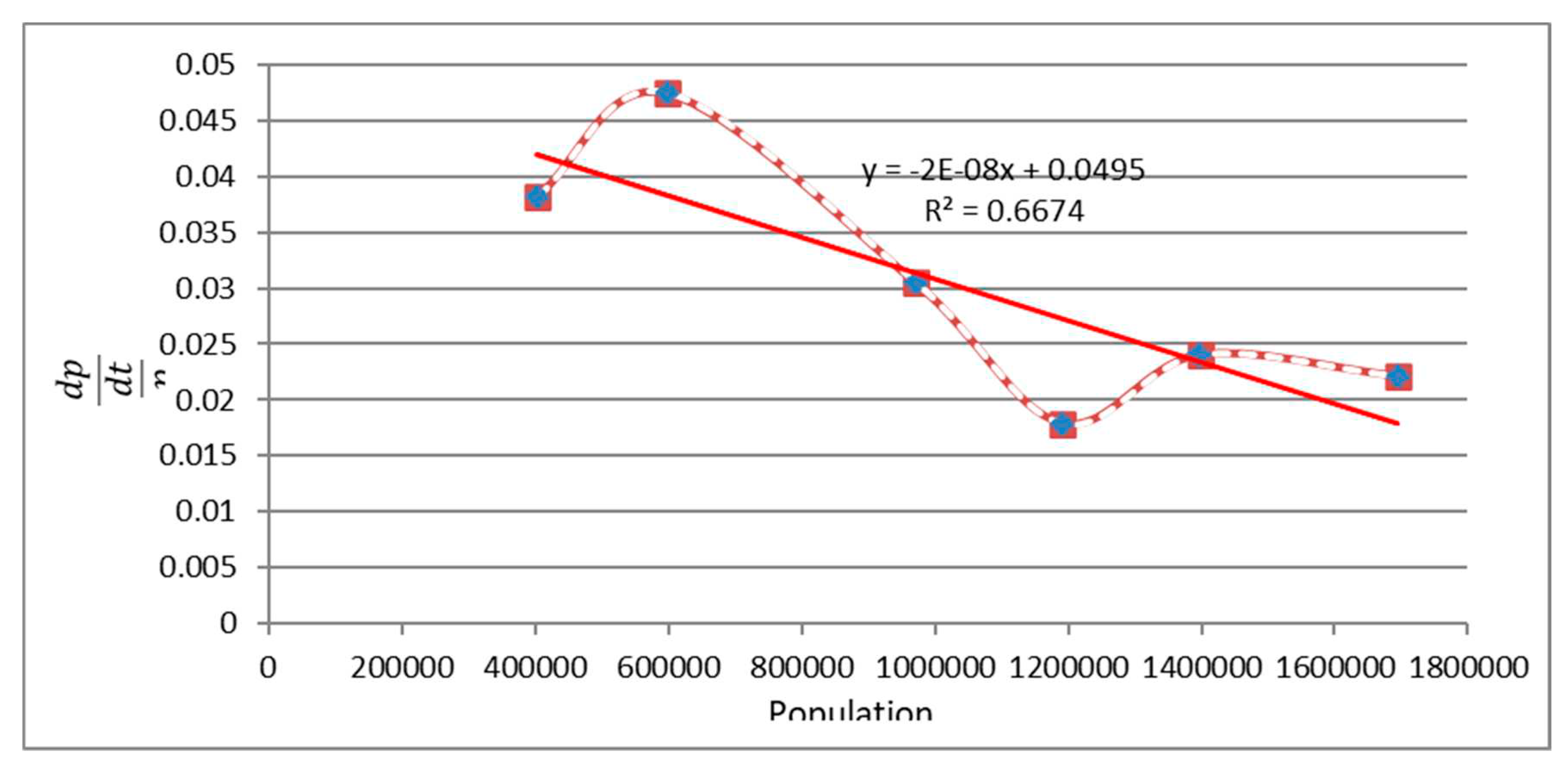
Figure 6 Shows the proportional growth rate (i.e. (dp/dt)/P ) versus the population number of Tabriz.
Table 2 represents the population of Tabriz during the years (eight distinct years). The values of proportional growth rate (i.e. (dp/dt)/P ) obtained in 1966, 1976,1986,1996,2006 and 2011 years, are shown in the fourth column. The slop dp/dt at a given year t is approximated by the slope of the line joining the pointes n years earlier and n years later. For example, the growth rate dp/dt in 1966 can be approximate by [P(1976)-P(1956)]/20 ). So, the value of calculated dp/dt are shown in the third column of
Table 1. By fitting the best line to the points, the value of R^2 was calculated to be 0.6674. The intercept and slope of the fitted line were calculated to be 0.0495 and -2×10^(-8) , respectively. Therefore, it can be concluded that the following formula for Tabriz city holds:
This implies that the value of r in Logistic equation is equal to intercept, i.e. r=0.0495. As the slope of the fitted line is equal to (-r )/k in Logistic equation, so it can be suggest that (-r)/k=-2×10^(-8) and k is equale to 2475000.
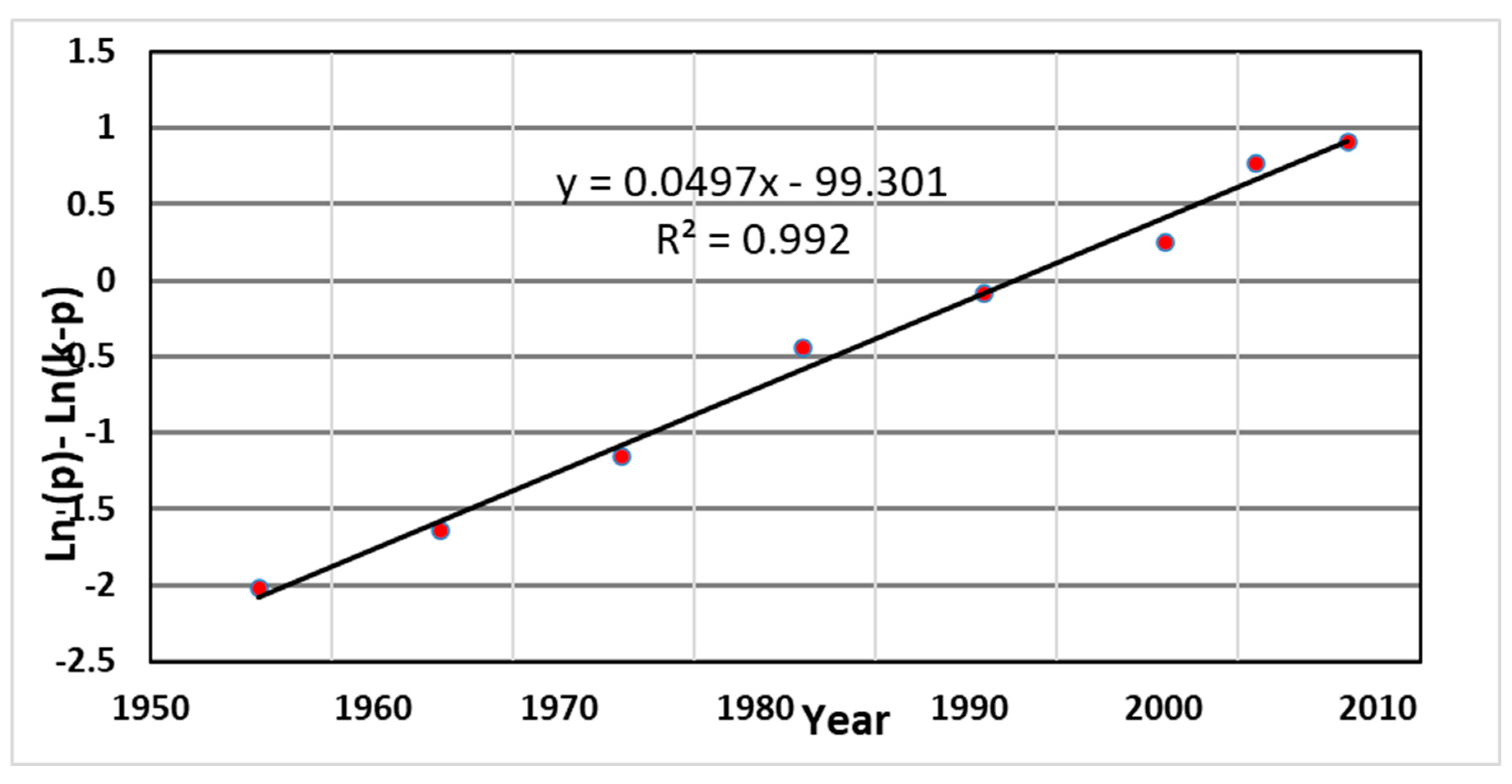
K in logistic growth model is the carrying capacity or maximum supportable population. By plotting ratios of dp/(dt/p) versus the populations p for testing logistic function based on actual population data of Tabriz city, it was found that the plot is roughly linear. However, only roughly and we obtained the value of the parameters of r and k based on this plot. Nevertheless, for better validation, it is necessary to use other fitting methods for testing. For this purpose, as can be seen from the equation i.e. (l n(p)-ln〖(k-p))〗=rt+c) resulted from equation (3), the term (l n(p)-ln(k-p)) is a linear function of t. The slope of the line is r. Thus, given the obtained value of K i.e. (2475000), the term (ln(p)-ln(k-p)) against t was plotted for Tabriz and shown in
Figure 7. It can be seen that the points seems to be on straight line.
Table 3 shows the value of (ln(p)-ln(k-p)) versus t, by using k is equal to 2475000 in Tabriz. By plotting the (l n(p)-ln(k-p)) against t (
Figure 8) and fitting the best line for observations, the more accurate value of r resulted (i.e. r=0.0497 ). The coefficient of determination for this fitting was equal to R^2=0.992.
Table 2.
Values of (l n(p)-ln(k-p)) in different years from 1956 to 2016 in Tabriz.
Table 2.
Values of (l n(p)-ln(k-p)) in different years from 1956 to 2016 in Tabriz.
| Year(t) |
Population(p) |
ln(p)-ln(k-p) |
| 1956 |
289996 |
-2.024072018 |
| 1966 |
403413 |
-1.640925011 |
| 1976 |
597976 |
-1.149205645 |
| 1986 |
971482 |
-0.443369281 |
| 1996 |
1191043 |
-0.082875571 |
| 2006 |
1398060 |
0.251719153 |
| 2011 |
1695094 |
0.763579524 |
| 2016 |
1773033 |
0.912415356 |
Then by using equation (m=-0.00000002=(-r/K)) and r=0.0497, we have:
Which yields the more accurate value of k (i.e. 2485000 for Tabriz).
It must be emphasized, we determined the reasonableness of a Logistic function fit for growth of population in Tabriz city up to 2016 by testing two methods in the fitting. In addition, parameters r and k have been estimated by using differential equations. By setting constant values (p_0=289996,r=0.0497,and k=2485000) in equation (P=(kp_0)/(p_0+(k-p_0)e^(-rt) )) (resulted from equation (3) symbolically), the following equation obtained for Tabriz city.
Where, p(t) is population of city in a year t. Therefore, we can predict the future population of Tabriz city based on the above equation (Logistic model) and the exponential model that from 2018 to 2100.
Table 3 and
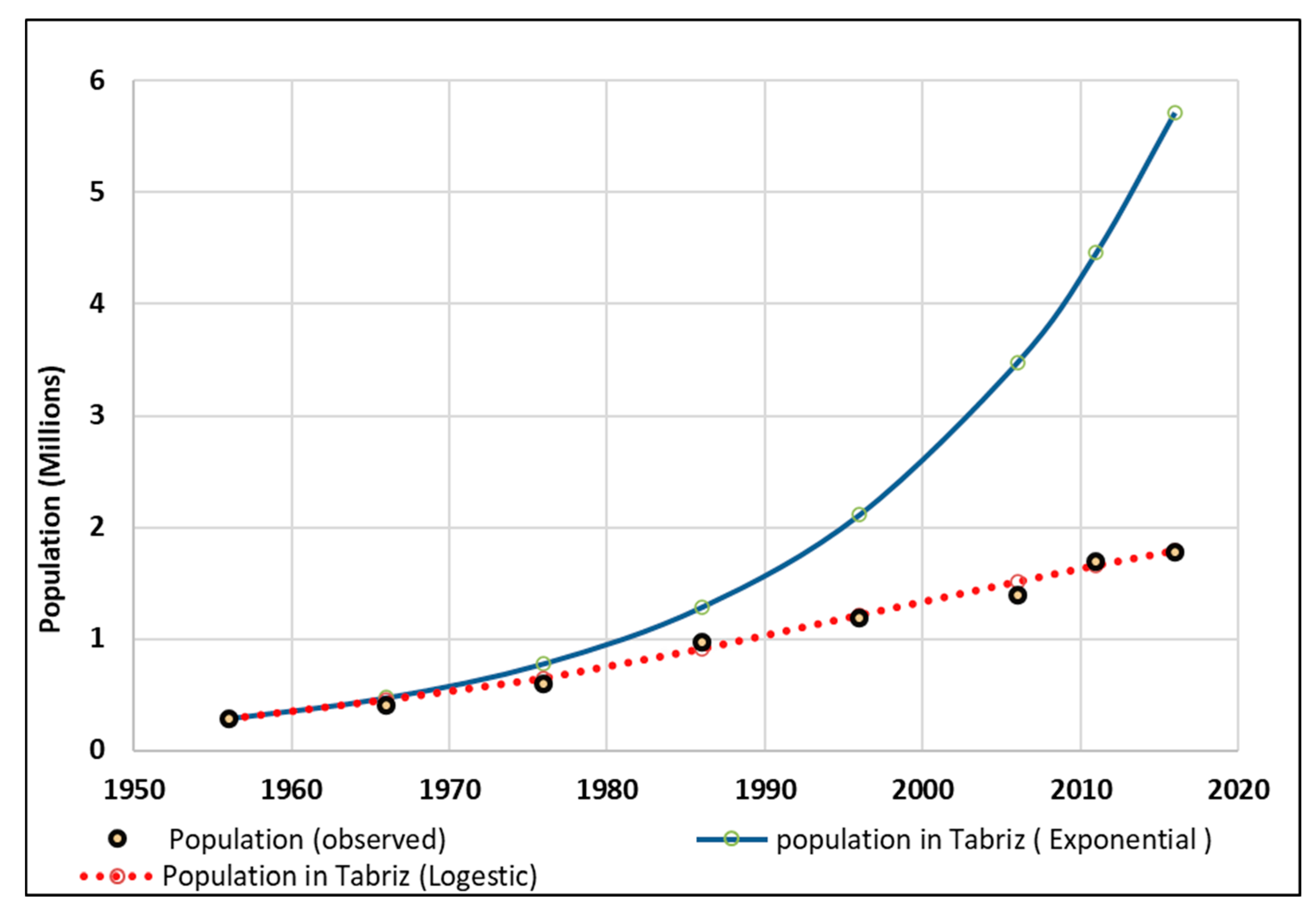
Table 4 show the observed and calculated values of population using the Logistic and Exponential models respectively. The MAPE calculated for Logistic and Exponential models were shown in the last column of these tables. As can be seen from the tables the maximum MAPE value for the logistic function is equal to be 4.8%. However, this value for exponential model was equal to 85.64%. The comparison of the obtained absolute percentage errors shows that the absolute error rate is acceptable for the logistic function, because, it is less than 5%. But, it is unacceptable for the exponential function because it is much more than 5%.
Figure 8 shows the observed and calculated population of Tabriz in the historical time (1956-2016) using the Logistic and Exponential models in Tabriz.
As it can be seen from
Figure 8, the actual population is perfectly fitted by Logistic model. But, it isn't fitted by exponential model. Also, it can be concluded that the population growth of Tabriz city has been out of the Exponential model and turned into the Logistic model since 1975.
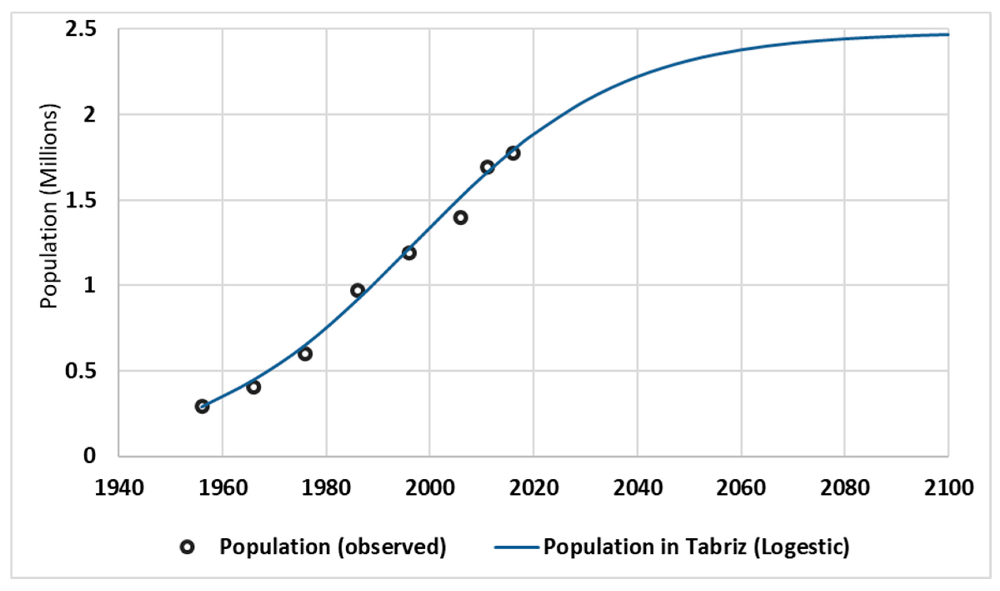
Figure 9 shows the observed and predicted population of Tabriz using the Logistic model. As it is clear from
Figure 9, the maximum possible population of Tabriz will be approximately reach to 2,500,000 by the 2100 year. It must also emphasize that this prediction can be a basis for planning in different dimensions, including water supply infrastructure and other needs in Tabriz city.
3.2. Inflection point and concavity in Logistic growth model
By simplifying equation 3, the following equation can be obtained.
The second derivative with respect to time led to follows:
By putting the value of dp/dt from (24) in (25), it can be write:
After some simplification, we have:
By setting equation (27) equal to zero, we can calculate value Inflection Points and Concavity by equation (28)
By simplifying equation (28), equation (29) is resulted.
With respect to k=2485000 for Tabriz city we have:
Two roots of above equation are:
p_1 and p_2 are the two inflection points. At these two points, the concavity of Logistic function curve (
Figure 9) changed. Therefore, by substituting the values of p_1 and p_2 to p(t) in equation (23) the time population reach to p_1 and p_2 are found.
the two answers are:
where t_1=40.73 and t_2 are the times of inflection points and concavity of Logistic curve respectively Tabriz city (
Figure 9). It can be concluded that the population growth of Tabriz has been changed and its sporadic growth decreased. In addition, direction of the population growth curve can be changed once the population of Tabriz reaches to its maximum possible value (i.e. 2100). Of course, this forecast will become true if the government policies on encouraging family’s children not changed. Obviously, current and future (until 2100) conditions in Tabriz city assumed to be same as the past.
3.3. Population and water consumption
It is clear that as population of a city increases the water consumption increases as well. To find the magnitude of correlation between population and water consumption in Tabriz city based on Pearson correlation test, it is need to test normality of water consumption data (Helsel et al., 2020). Results of normality tests are shown in
Table 5. It can be concluded that water consumption data follows normal distribution in all sections except the educational, religious and free water. The Pearson's correlation coefficient is not calculated for the mentioned two sections. Therefore, according to the tests of normality and attention to this issue, correlation coefficients in three methods including Pearson, Spearman's Rho and Kendall's rank coefficients have been calculated for water consumption data series and have been showed in
Table 6. For calculation Pearson Correlation coefficient and Spearman's Rho rank coefficient, we used free online statistics software that is available online from (
https://www.socscistatistics.com). Also, for calculation Kendall's rank coefficient, we used other free online statistics software that is available online from (Wessa, 2022).
The results shown in
Table 6 indicates that the amount of water consumption in all sections in Tabriz city are strongly correlated with population number from 2012 to 2021. In addition, there is a high positive correlation between the total and household water consumption with population in Tabriz city. This important result will be used in prediction of future water demand later.
3.4. Prediction of water consumption
Water demand in Tabriz city was predicted using the linear and quadratic models. As, the skewness of total water consumption data was 0.284607, (and non-significant at 5% level). Therefore, the data approximately is symmetric distributed. Therefore, the OLS estimation was used to prediction of parameters.
3.4.1. Linear trend analysis of total water consumption
Results showed that the values parameters are of γ_1=0.0000509 and γ_0=16.72031. Therefore, the trend line equation for demand is as follows:
Where,
d : Water demand volume (in millions of cubic meters). And
p: Population number.
Table 7 shows the output of ANOVA in water demand of Tabriz as a function of population number.
As can be seen from
Table 2, the F-ratio value is 5905.3. The P_- value is <0.00001, Therefore, the result is significant at <0.05 . It can be concluded that, the null hypothesis (i.e. the slope is equal to zero) is rejected and the alternative hypothesis (i.e. the slop is not equal to zero) accepted at 0.05 level. Based on the OLS procedure, it can be concluded that there is a significant positive trend in total water demand in Tabriz city as indicated by the positive γ_1=0.0000509.
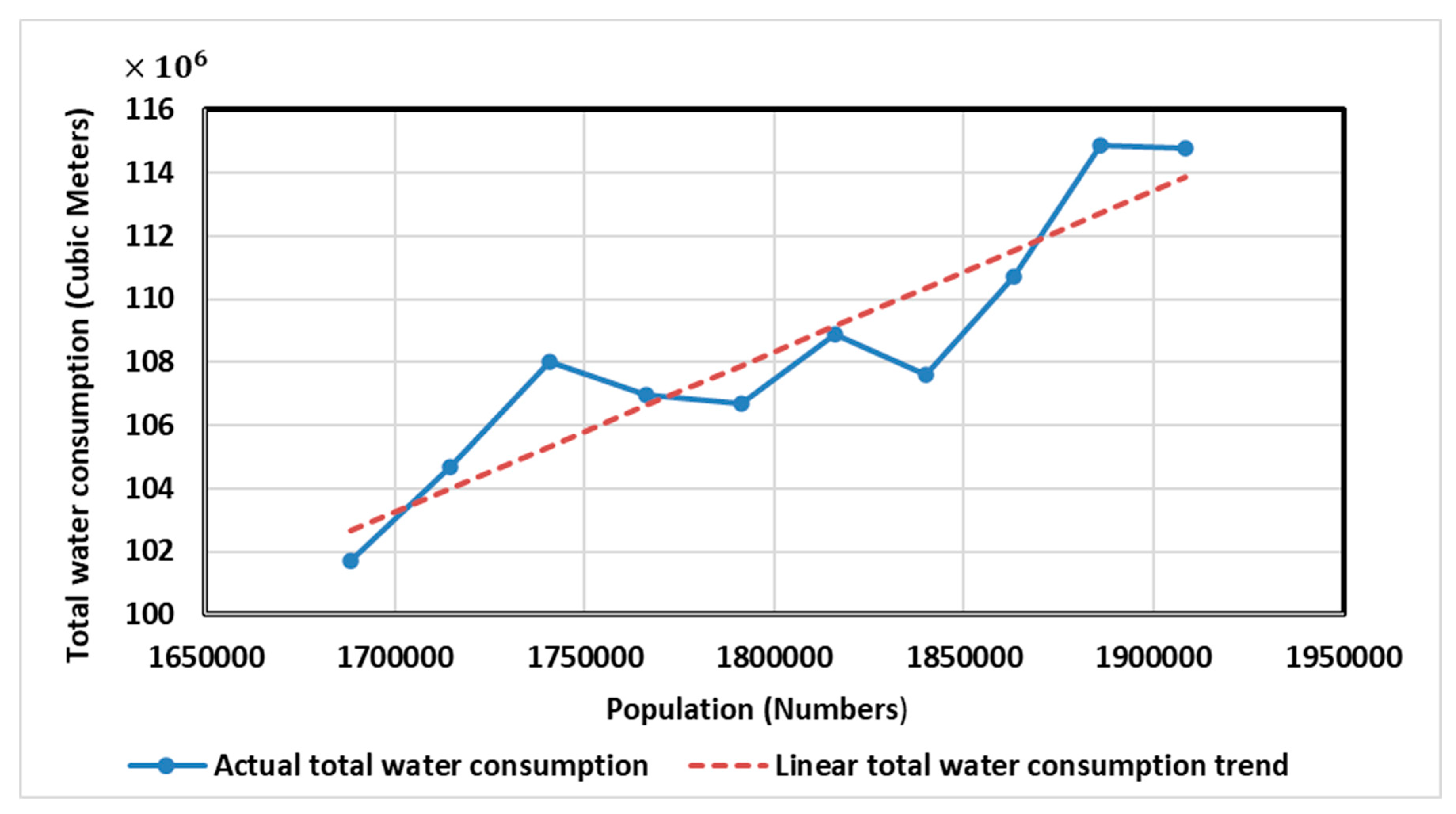
Figure 10 shows the liner trend plot of the total water consumption in Tabriz city in the historical period (2012-2021).
3.4.2. Quadratic trend analysis for total water consumption
Employing the quadratic model for total water consumption to Tabriz population in equation (9) and (10), the obtained parameters are:
γ_1=-0.0002967, γ_0=328.9 and γ_2=0.00000000009663.
As a result, the quadratic trend function is:
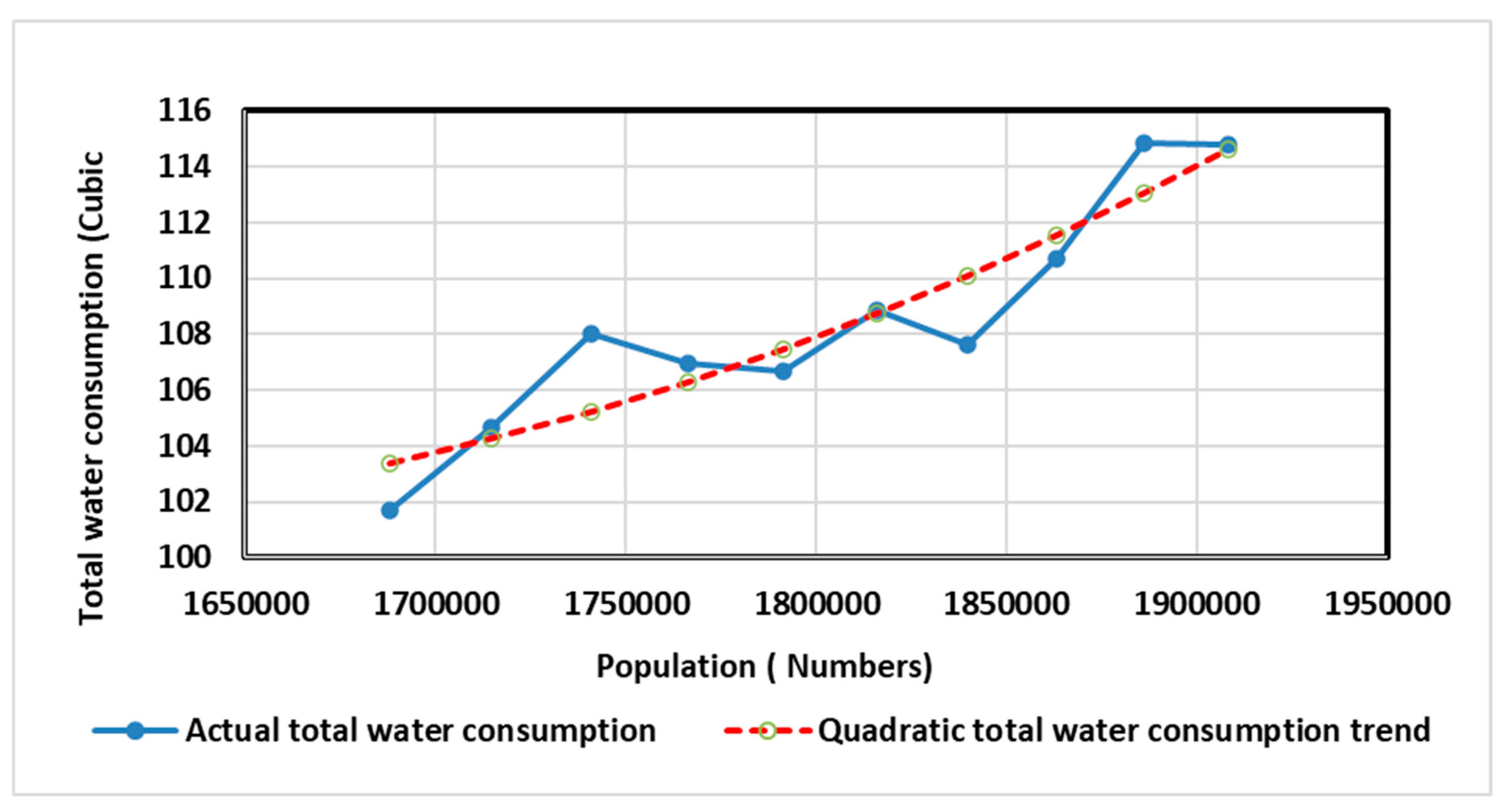
Table 8 represents the ANOVA output using the quadratic form of the trend analysis. In addition,
Figure 11 indicates Fitting quadratic form of trend line for total water consumption in Tabriz (2012-2021).
The OLS results shown in
Table 8 indicated that both the linear and quadratic terms were significantly significant, i.e. different from zero, at 0.05 level.
3.4.3. Comparison between the linear trend and Quadratic trend
To determine which trend model best fits the total water consumption in Tabriz city; the mean absolute percentage error (MAPE %), Mean Absolute deviation (MAD) and Mean Square Deviation (MSD) were calculated. Results of assessment criteria are summarized in
Table 9. As can be seen from
Table 9, the assessing measures for both liner and quadratic form of trends are similar to each other. Although, the linear trend is preferable due to parsimony of parameters.
3.5. Analysis of water scarcity
Bearing in mind the available urban water, the urban water stress is calculated from 2012 to 2100.
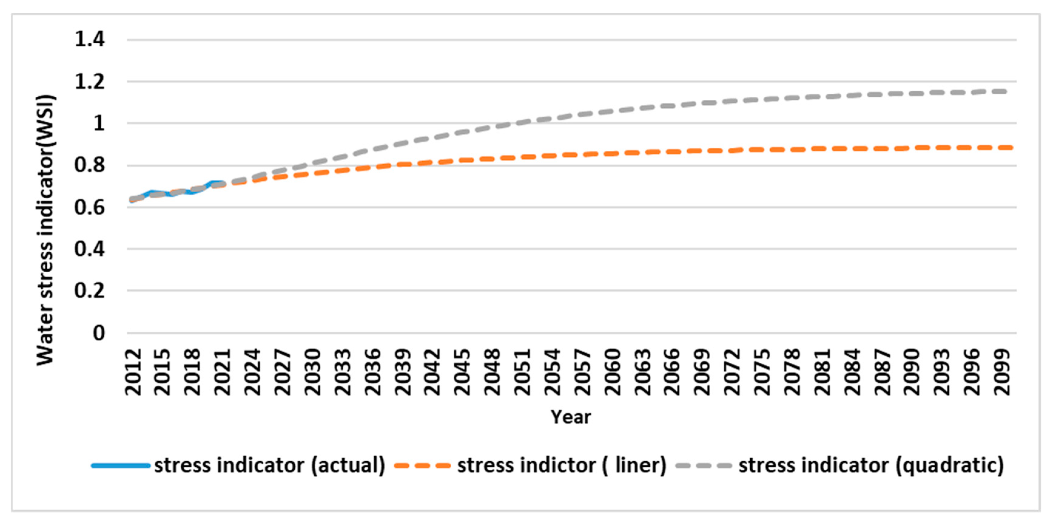
Figure 12 shows the water stress in the future period for Tabriz. Both the linear and quadratic form of water demands were used here. As can be seen from
Figure 13 [M2] that both of the models showed increasing water stress in future period. However, quadratic form estimate water stress more than the linear trend. Both the models start water stress measure from 0.62 in 2012. In linear model, water stress measure reach to more than 0.8 in 2100. Nevertheless, water stress measure approximately reach to 1.2 in quadratic model in 2100.
Figure 12 illustrates the water stress indicator during the future period (2012 to 2021) using the linear and quadratic trend models in Tabriz city. According to
Figure 12 in 2050, the water stress index will reach to more than 0.8 (WSI>0.8) in the linear model. However, this index exceeds 1 using the more than 1 in quadratic model. In addition, it is clear that by such an increasing trend in urban water consumption, it is true the time in which city encountered with water stress in 2050. Even, the effect of climate changes ignored. According to Falkenmark et al. (1989) classification, the water stress in the beginning year (2012) is in high and rises to higher levels later. As a result, water shortage in Tabriz city accelerated year to year by changing climate, increasing the city population and developing the industrial factories.
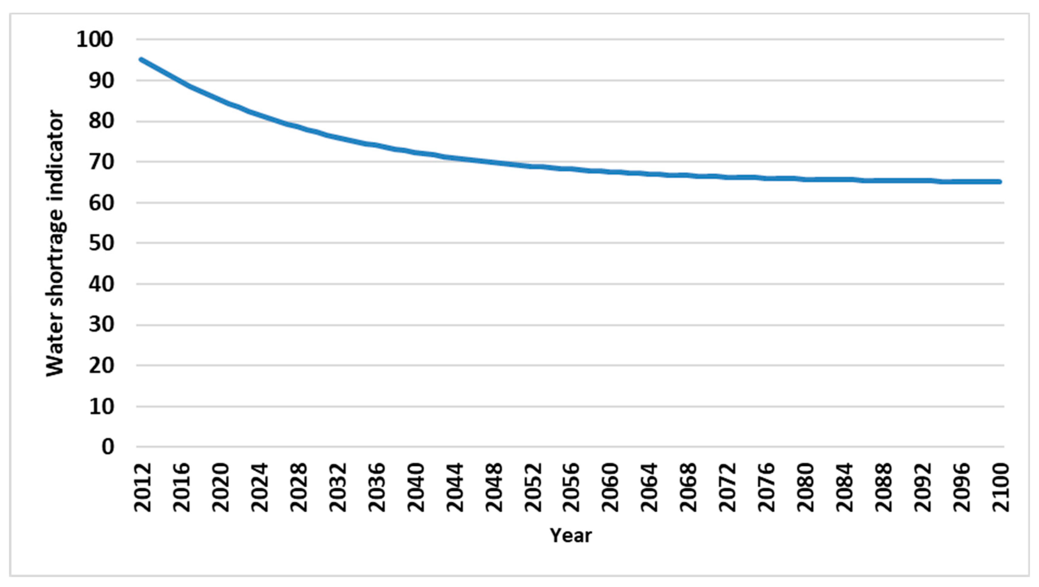
Figure 13 demonstrates the water shortage indicator from 2012 to 2100 in Tabriz city. As can be shown from the
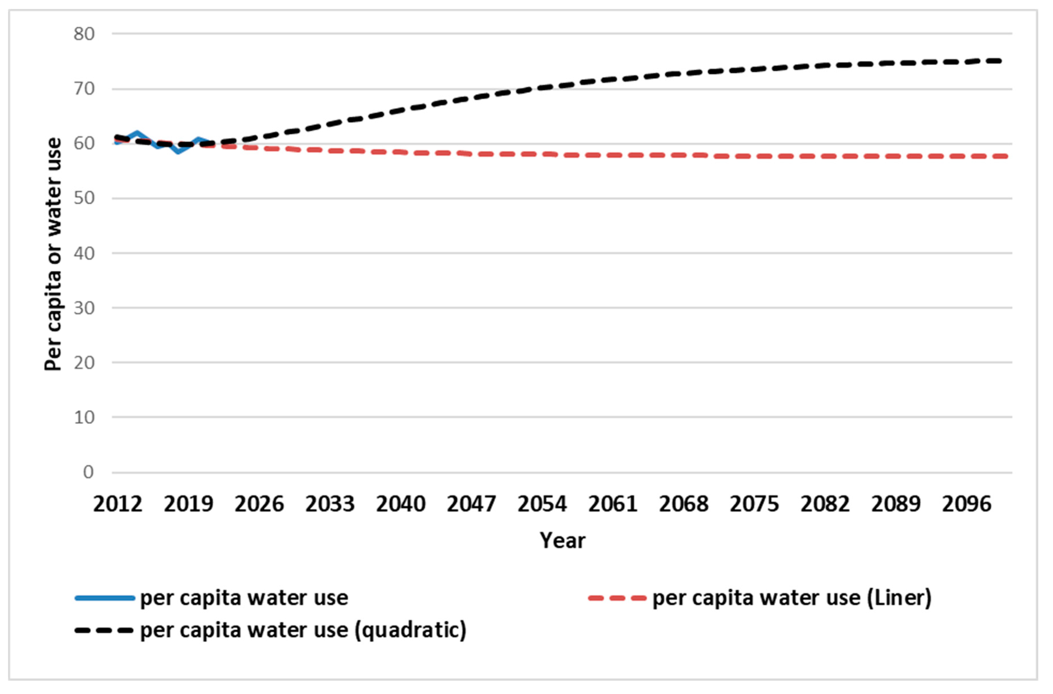
Figure 14 trends in water shortage index is decreasing in this city. This index will be declined to less than 70 (WCI<70) in 2050. According to Falkenmark et al. (1989) classification, the water shortage index in the beginning year (2012) is in high level. It will be rose to higher levels in the future years at Tabriz. This means that decision makers will be faced to critical conditions later. Especially, it can be emphasized that the trends in per capita water consumption in Tabriz city is upward using the quadratic trend model (
Figure 11). In the case of the linear model, it follows almost a constant trend (
Figure 10). Because, the rate of increase in water consumption in linear model is less than the quadratic model.
Figure 14 shows the per capita of water consumption in Tabriz using the linear and quadratic models (2012-2100). In general, it can be concluded that per capita water consumption affect urban water consumption, water stress index and water shortage in Tabriz. By increasing the rate of water use per capita, the index of water stress increases. However, the water shortage decreases simultaneously. In addition, as time passes, the water shortage become more perceptible. Therefore, urban water decision-makers try to reduce it with various incentive methods and adopting limiting decisions in Tabriz city. Nevertheless, for various reasons, including health, cultural, social, economic, even political issues, as well as climate changes, this issue has not be happened.
4. Conclusions
This study showed that Tabriz population growth rate followed on exponential model from 1956 to 1975. Nevertheless, from 1975 later due to various reasons such as economic, social, cultural, political and so on, population growth pattern turned to be a Logistic function model. Results indicated that the amount of water consumption would be increased proportional with population growth. Decision makers and experts should be considered the population growth of Tabriz in future years in terms of drinking water, scientific planning for drainage infrastructure, purification structures and so on. Using the two linear and quadratic population growth models in Tabriz, the amount of water urban demand in future years was calculated. Results indicated that the water stress and shortage indexes in Tabriz gradually accelerated in future years. In quadratic water demand model, the per capita consumption of water per person will be increase in the Tabriz city. Nevertheless, in the linear water demand model, the per capita water consumption follows an almost constant pattern in the Tabriz city. Of course, urban water demand might be increased not only due to population increase but also due to several other reasons such as climate change, various infectious diseases such as Covid 19, urban development, industrial development, rising level of sanitation and so on. This research introduced a new perspective for other researchers to conduct similar study in other large cities. In addition, by using the used method, it is possible to better plan for the future of cities in terms of population growth, water demand and consumption, water shortage and water stress and in general for water security.
Internet references:
Availability of Data and Materials
Acknowledgments
This work is based upon research funded by Iran National Science Foundation (INFS) under project No. 4013231, which is appreciated. Historical data of urban water consumption provided by Water and Wastewater Company of Tabriz, which is greatly acknowledged.
References
- Andongwisye JM, Allen RM, (2019) Mathematical model for Tanzania population growth. Tanzan J. of Science, 45(3), 346-354. Available online: https://tjs.udsm.ac.tz/index.php/tjs/article/view/201.
- Al-Eideh BM, Al-Omar HO, (2019) Population projection model using exponential growth function with a birth and death diffusion growth rate processes. European J. of Scientific Res.151 (3), 271-276.
- Boreti A, Lorenzo R, (2019) Reassessing the projections of the world water development report. NPJ Clean Water. 2 (1), 1–6. ISSN 2059-7037. [CrossRef]
- Brika B, (2019) The water crisis in Libya: causes, consequences and potential solutions. Desalination and Water Treatment, 167, 351–358. [CrossRef]
- Capt T, Mirchi A, ASCE AM, Kumar S, ASCE M, Shane Walker W, (2021) Urban water demand: statistical optimization approach to modeling daily demand, J. of Water Resources Planning and Management, 147(2), 1-10.
- Cohen JE, (1995) Population growth and earth’s human carrying capacity. Science, 269 (5222), 341-346.
- Cooper B, Burton M, Crase L, (2011) Urban water restrictions: Attitudes and avoidance. Water Resources Res. 47, 1-13. [CrossRef]
- Di Mauro A, Cominola A, Di Nardo A, Castelletti A, (2021) Urban Water Consumption at Multiple Spatial and Temporal Scales, a Review of Existing Datasets. Water, 13, 36. [CrossRef]
- Eslamian S, (2014) Handbook of Engineering Hydrology: Environmental Hydrology and Water Management. Boca Raton, Florida: CRC Press. p. 89. ISBN 978-1-4665-5249-4.
- Falkenmark M, Lundqvist J, Widstrand C, (1989) Macro-scale water scarcity requires micro-scale approaches. Natural Res. Forum, 13 (4), 258–267. ISSN 1477-8947. [CrossRef]
- Fielding KS, Russell S, Spinks A, Mankad A, (2012) Determinants of household water conservation: The role of demographic, infrastructure, behavior, and psychosocial variables. Water Resources Res. 48, 1-12. [CrossRef]
- Gesusldo GC, Oliveira PT, Rodrigues DBB, Gupta HV, (2019) Assessing water security in the Sao Paulo city region under projected climate change. Hydrology and Earth System Sciences. 23, 4955-4956. [CrossRef]
- Ginkel KCHV, Hoekstra AY, Buuman J, Hogeboom RJ, (2018) Urban Water Security Dashboard: Systems Approach to Characterizing the Water Security of Cities. Water Resource Planning Management. 12, 1-11.
- Glass N, (2010) The Water Crisis in Yemen: Causes, Consequences. Global Majority E-J. 1(1), 17-30. Available online: https://www.american.edu/cas/economics/ejournal/upload/glass_accessible.pdf.
- Gupta SP, (2005) Statistical Methods, Sultan Chand and Sons Educational Publishers, New Delhi.
- Hathout D, (2013) Modeling population growth: exponential and hyperbolic modeling, applied mathematics. 4, 299-304. [CrossRef]
- Helsel DR, Hirsch RM, Ryberg KR, Archfield SA, and Gilroy EJ, (2020) Statistical methods in water resources: U.S. Geological Survey Techniques and Methods, book 4, chap. A3, 458 p.[Supersedes USGS Techniques of Water-Resources Investigations, book 4, chap. A3, version 1.1.]. [CrossRef]
- Khatibi S, Arjjumend H, (2019) Water crisis in making in Iran. Grassroots J. of Natural Resources. 2(3), 45-54. [CrossRef]
- Karimi SS, Yasi M, Cox JP, Eslamian S, (2014) Case Study: Typical Rivers in Urmia Lake Basin, Iran.
- Kummu M, Guillaume JHA, Moel Hde, Eisner S, Flörke M, Porkka M, Siebert S, Veldkamp, TI E, Ward PJ, (2016) The world’s road to water scarcity: shortage and stress in the 20th century and pathways towards sustainability. Scientific reports 6 (1), 1-16.
- Lipkin L, Smith D, (2004) Logistic Growth Model. Available online: https://www.maa.org/press/periodicals/loci/joma/logistic-growth-model-background-logistic-modeling.
- Liu Y, Miao Y, Xiaoyi M, Xing X, (2017) Estimating models for reference evapotranspiration with core metrological parameters via path analysis. Hydrology Research. 48(2):340-354.
- Liu J, Yang H, Gosling SN, Kummu M, Flörke M, Pfister S, Hanasaki N, Wada Y, Zhang, X, Zheng C, Alcamo J, Oki T, (2017) Water scarcity assessments in the past, present, and future. Earth’s Future. 5, 545–559. [CrossRef]
- Maftei C, Barbulescu A, (2008) Statistical Analysis of Climate Evolution in Dobrudja Region. Proceedings of the World Congress on Engineering. London, U.K.
- Machiwal D, Jha MK, (2008) Cooperative evaluation of statistical tests for time series analysis: Application to hydrological time series. Hydrological Sciences J., 53(3), 353–366. [CrossRef]
- Mekonnen MM, Hoekstra AY, (2016) Four billion people facing severe water scarcity. Science Advances, 2(2), 1-7.
- Murgatroyd A, Charles KJ, Chautard A, Dyer E, Grasham C, Hope R, Hoque SF, Water Security for Climate Resilience Report: A synthesis of research from the Oxford University REACH programme. University of Oxford, 2021.
- Korzenevica M, Munday C, Alvarez-Sala J, Dadson S, Hall JW, Kebede S, Nileshwar A, Olago D, Salehin M, Ward F, Washington R, Yeo D, Zeleke G, (2021) Water Security for Climate Resilience Report: A synthesis of research from the Oxford University REACH programme. University of Oxford, UK: REACH. Available online: https://reachwater.org.uk/wp-content/uploads/2021/08/REACH-climate-summary.pdf.
- Muller M, (2017) Cape Town’s water crisis. Civil Engineering, 11-16. Electronic copy. Available online: https://ssrn.com/abstract=2995937.
- Moridi A, (2017) State of water resources in Iran. International J. Hydrology, 1(4), 111‒114. [CrossRef]
- Nyamao Nyabwanga R, Ouko Otumba E, Onyango F, Otieno S, (2015) Statistical trend analysis of residential water demand in Kisumu City, Kenya, American J. of Theoretical and Applied Statistics, 4(3), 112-117. [CrossRef]
- Padowski JC, Jawitz JW, (2011) Water availability and vulnerability of 225 large cities in the United States. Water Resources Research, 48, W12529.
- Saatsaz M, (2020) Ahistorical investigation on water resources management in Iran. Environ. Development and Sustainability, 22(3), 1749–1785. [CrossRef]
- Shapiro SS, Wilk MB, (1965) An analysis of variance test for normality (Complete Samples). Biometrika, 52(3-4):591-611.
- Sue J, Lesley H, (2020) Australia’s mass fish kills as a crisis of modern water: Understanding hydro social change in the Murray-Darling Basin. Geoforum. 109, 44-56. ISSN 0016-7185. [CrossRef]
- Tolba Abelnga H, El-Naser H, Ribbe L, Frechen FB, (2022) Assessing water security in water-scarce cities: Applying the integrated urban water security index (IUWSI) in Madaba, Jordan. Water, 12(5), 1299. [CrossRef]
- Ullrich PA, Xu Z, Rhoades AM, Dettinger MD, Mount JF, Jones AD, Vahmani P, (2018) California’s Drought of the Future: A Midcentury Recreation of the Exceptional Conditions of 2012–2017. Earth’s Future. 6, 1568-1587.
- Unicef, (2021) Urban water scarcity guidance note report, 1-35. Available online: https://www.unicef.org/media/95381/file/Urban-Water-Scarcity-guidance-note.pdf.
- Vinkatasha P, Blessy G, Sachy E, Akshaya B, Arya Kumari S, (2017) Mathematical Modelling of Population Growth. International J. of Science, Engineering and Management (IJSEM), 11,117-121. Available online: https://www.technoarete.org/common_abstract/pdf/IJSEM/v4/i11/Ext_71403.pdf.
- Vörösmarty CJ, Green P, Salisbury J, Lammers RB, (2000) Global water resources: vulnerability from climate change. Science, 289, 284-288. [CrossRef]
- Wessa P, (2022) Free Statistics Software, Office for Research Development and Education, version 1.2.1. Available online: https://www.wessa.net/.
Figure 1.
Development of high-rise buildings in Tabriz city (photo is for 2022).
Figure 1.
Development of high-rise buildings in Tabriz city (photo is for 2022).
Figure 2.
The schematic representation of the water resources of Tabriz city (Zarghami and Akbariyeh, 2012).
Figure 2.
The schematic representation of the water resources of Tabriz city (Zarghami and Akbariyeh, 2012).
Figure 3.
Histogram of urban water consumption at Tabriz city in (2012 to 2021). (a) Total and Household urban water consumption; (b) sectional water consumption.
Figure 3.
Histogram of urban water consumption at Tabriz city in (2012 to 2021). (a) Total and Household urban water consumption; (b) sectional water consumption.
Figure 4.
The Flowchart of the present study.
Figure 4.
The Flowchart of the present study.
Figure 5.
The pattern of Exponential (upper curve) and Logistic (lower curve) population growth curve models. Note: P (Population), t (time) and K (carrying capacity also called maximum supportable population).
Figure 5.
The pattern of Exponential (upper curve) and Logistic (lower curve) population growth curve models. Note: P (Population), t (time) and K (carrying capacity also called maximum supportable population).
Figure 6.
Relative ratios of dp/(dt/p) versus the population number according to historical population of Tabriz City.
Figure 6.
Relative ratios of dp/(dt/p) versus the population number according to historical population of Tabriz City.
Figure 7.
Plotting the term (l n(p)-ln(k-p)) against t for better validation in testing Logistic function based on observed data of Tabriz city.
Figure 7.
Plotting the term (l n(p)-ln(k-p)) against t for better validation in testing Logistic function based on observed data of Tabriz city.
Figure 8.
Actual and predicted population using the Logistic and Exponential models from 1956 to 2016 in Tabriz city.
Figure 8.
Actual and predicted population using the Logistic and Exponential models from 1956 to 2016 in Tabriz city.
Figure 9.
Actual and predicted population using the Logistic model from 1956 to 2100 in Tabriz city.
Figure 9.
Actual and predicted population using the Logistic model from 1956 to 2100 in Tabriz city.
Figure 10.
Historical total water consumption as a population number in Tabriz.
Figure 10.
Historical total water consumption as a population number in Tabriz.
Figure 11.
Fitting quadratic form of trend line for total water consumption in Tabriz (2012-2021).
Figure 11.
Fitting quadratic form of trend line for total water consumption in Tabriz (2012-2021).
Figure 12.
Water stress indicator in both linear and quadratic trend model in Tabriz city (2012 to 2021).
Figure 12.
Water stress indicator in both linear and quadratic trend model in Tabriz city (2012 to 2021).
Figure 13.
Water shortage indicator in Tabriz city (2012 to 2100).
Figure 13.
Water shortage indicator in Tabriz city (2012 to 2100).
Figure 14.
Per capita water use indicator using linear and quadratic population growth models from 2012 to 2100 in Tabriz city.
Figure 14.
Per capita water use indicator using linear and quadratic population growth models from 2012 to 2100 in Tabriz city.
Table 1.
Population number (p) from 1956 to 2016 according to the census of the Statistical Organization of Iran and the ratio of dp/dt to p in Tabriz City.
Table 1.
Population number (p) from 1956 to 2016 according to the census of the Statistical Organization of Iran and the ratio of dp/dt to p in Tabriz City.
| Year(t) |
Population(p) |
|
|
| 1956 |
289996 |
- |
- |
| 1966 |
403413 |
15399 |
0.038172 |
| 1976 |
597976 |
28403.45 |
0.047499 |
| 1986 |
971482 |
29653.35 |
0.030524 |
| 1996 |
1191043 |
21328.9 |
0.017908 |
| 2006 |
1398060 |
33603.4 |
0.024036 |
| 2011 |
1695094 |
37497.3 |
0.022121 |
| 2016 |
1773033 |
- |
- |
Table 3.
Observed and predicted population number and MAPE% using the Logistic model in Tabriz city.
Table 3.
Observed and predicted population number and MAPE% using the Logistic model in Tabriz city.
| Year (t) |
Observed (P) |
Predicted (P) |
MAPE% |
| 1956 |
289996 |
289996 |
0.00 % |
| 1966 |
403413 |
442828 |
4.89 % |
| 1976 |
597976 |
652269 |
6.28 % |
| 1986 |
971482 |
916321 |
6.13 % |
| 1996 |
1191043 |
1216326 |
5.33 % |
| 2006 |
1398060 |
1519414 |
5.89 % |
| 2011 |
1695094 |
1661045 |
5.33 % |
| 2016 |
1773033 |
1791386 |
4.80 % |
| 2020 |
|
1886032 |
|
| 2030 |
|
2082121 |
|
| 2040 |
|
2222935 |
|
| 2050 |
|
2318468 |
|
| 2060 |
|
2380808 |
|
| 2070 |
|
2420461 |
|
| 2080 |
|
2445275 |
|
| 2090 |
|
2460644 |
|
| 2100 |
|
2470104 |
|
Table 4.
Observed (1956-2016) and predicted (2020-2100) population number and MAPE% using the Exponential model in Tabriz city.
Table 4.
Observed (1956-2016) and predicted (2020-2100) population number and MAPE% using the Exponential model in Tabriz city.
| Year(t) |
Observed (p) |
Population (p) |
MAPE% |
| 1956 |
289996 |
289996 |
0.00 % |
| 1966 |
403413 |
476690 |
8.99 % |
| 1976 |
597976 |
783575 |
16.21 % |
| 1986 |
971482 |
1288027 |
20.15 % |
| 1996 |
1191043 |
2117237 |
31.46 % |
| 2006 |
1398060 |
3480277 |
50.73 % |
| 2011 |
1695094 |
4462066 |
66.49 % |
| 2016 |
1773033 |
5720818 |
85.64 % |
| 2020 |
|
6979043 |
|
| 2030 |
|
11472029 |
|
| 2040 |
|
18857521 |
|
| 2050 |
|
30997664 |
|
| 2060 |
|
50953418 |
|
| 2070 |
|
83756338 |
|
| 2080 |
|
137677205 |
|
| 2090 |
|
226311383 |
|
| 2100 |
|
372006695 |
|
Table 5.
Results of PPCC and Shapiro-Wilk normality tests employing the water consumption data from 2012 to 2021 in Tabriz city.
Table 5.
Results of PPCC and Shapiro-Wilk normality tests employing the water consumption data from 2012 to 2021 in Tabriz city.
| section |
R |
S-W |
n |
Region of acceptance |
Result |
| Household |
0.96258 |
0.9181 |
10 |
%95 |
normal |
| Industrial |
0.9573 |
0.8922 |
10 |
%95 |
normal |
| Commercial |
0.9875 |
0.9734 |
10 |
%95 |
normal |
| Public and governmental |
0.9664 |
0.9356 |
10 |
%95 |
normal |
| Educational and religious |
0.8669 |
0.746 |
10 |
%95 |
Non normal |
| Free water |
0.717 |
0.5448 |
10 |
%95 |
Non normal |
| Other |
0.9599 |
0.9216 |
10 |
%95 |
normal |
| Total |
0.9724 |
0.9429 |
10 |
%95 |
normal |
Table 6.
Results of correlation between population and water consumption in different sections using the three distinct methods employing the data from 2012 to 2021 in Tabriz city.
Table 6.
Results of correlation between population and water consumption in different sections using the three distinct methods employing the data from 2012 to 2021 in Tabriz city.
| Water consumption section |
PCC |
S- Rho |
KRC |
P-value(PCC) |
P-value(S- Rho) |
P-value (KRC) |
Correlation degree |
| Household |
0.9355 |
0.93939 |
0.822222 |
0.00007 |
0.00005 |
0.001282 |
Very high (positive) |
| Industrial |
-0.7237 |
-0.68485 |
-0.511111 |
0.01815 |
0.02888 |
0.049098 |
High (negative) |
| Commercial |
0.9312 |
0.87879 |
0.733333 |
0.0001 |
0.00081 |
0.004207 |
Very high (positive) |
| Public and governmenta |
-0.0982 |
-0.15152 |
-0.200000 |
0.07877 |
0.67607 |
0.474274 |
Very weak (negative) |
| Educational and religious |
-0.8148 |
-0.91515 |
-0.777777 |
0.004089 |
0.0002 |
0.0023575 |
Very high (negative) |
| Free water |
-0.3102 |
-0.70909 |
-0.466667 |
0.383048 |
0.02167 |
0.073638 |
Weak (negative) |
| Other |
-0.5551 |
-0.39394 |
-0.2888889 |
0.095854 |
0.26 |
0.283131 |
Moderate (negative) |
| Total |
0.9177 |
0.87879 |
0.733333 |
0.000182 |
0.00081 |
0.004207 |
Very high (positive) |
Table 7.
ANOVA table for water consumption as a function of Tabriz population.
Table 7.
ANOVA table for water consumption as a function of Tabriz population.
| Source of variation |
df |
SS |
MS |
F-ratio |
| Regression |
1 |
16/224/201/181/431.1 |
16/224/201/181/431.1 |
|
| Error |
18 |
49/453/030/182.9 |
2/747/390/565.7 |
|
| Total |
19 |
16/273/654/211/614 |
|
|
Table 8.
The output of ANOVA using the quadratic form of trend analysis.
Table 8.
The output of ANOVA using the quadratic form of trend analysis.
| Parameter |
Parameter Estimates |
SE |
P-Value |
|
|
0.00021 |
|
|
|
0.0000 |
<0.001 |
|
|
0.0000 |
<0.001 |
Table 9.
Model accuracy measures for linear and quadratic form of trend analysis in Tabriz.
Table 9.
Model accuracy measures for linear and quadratic form of trend analysis in Tabriz.
| Trend model |
MAPE% |
MAD |
MSD |
| Linear trend |
1.17 |
3.04 |
12.81 |
| Quadratic trend |
1.09 |
3.13 |
13.01 |
|
Disclaimer/Publisher’s Note: The statements, opinions and data contained in all publications are solely those of the individual author(s) and contributor(s) and not of MDPI and/or the editor(s). MDPI and/or the editor(s) disclaim responsibility for any injury to people or property resulting from any ideas, methods, instructions or products referred to in the content. |
© 2023 by the authors. Licensee MDPI, Basel, Switzerland. This article is an open access article distributed under the terms and conditions of the Creative Commons Attribution (CC BY) license (http://creativecommons.org/licenses/by/4.0/).
