Risk Assessment of Power Supply Security Considering Electricity Facility Outages in Extreme Precipitation Scenarios

Preprint

Article

Risk Assessment of Power Supply Security Considering Electricity Facility Outages in Extreme Precipitation Scenarios

Altmetrics

Downloads

115

Views

Comments

A peer-reviewed article of this preprint also exists.

Gang Zhou,Jian-xun Shi,Bing-jing Chen,Zhong-yi Qi,

Li-cheng Wang^*

Gang Zhou,Jian-xun Shi,Bing-jing Chen,Zhong-yi Qi,

Li-cheng Wang^*

This version is not peer-reviewed

Submitted:

27 July 2023

Posted:

28 July 2023

You are already at the latest version

Alerts

Abstract

To quantitatively estimate the risk of power system operation under extreme rainfall, a multi-scenario stochastic risk assessment method is proposed. First, a scenario generation scheme considering waterlogged faults of power facilities is constructed based on the storm water management model (SWMM) and the extreme learning machine method. These scenarios will be merged to several typical scenario sets for further processing. The outage of power facilities will induce power flow transfer which may consequently lead to transmission lines’ thermal limit violation. Semi-invariant and Gram-Charlier level expansion methods are adopted to analytically depict the probability density function and cumulative probability function of each line’s power flow. The optimal solution is performed by a particle swarm algorithm to obtain proper load curtailment at each bus, and consequently the violation probability of line thermal violations can be controlled within an allowable range. The volume of load curtailment as well as their importance are considered to quantitatively access the risk of power supply security under extreme precipitation scenarios. The effectiveness of the proposed method is verified in case studies based on the IEEE 24-bus system.

Keywords:

Subject: Engineering - Electrical and Electronic Engineering

1. Introduction

With global warming in recent years, extreme natural disasters have occurred frequently [1]. This has led to a rising level of damage to power systems and induce huge economic losses [2]. Hereinto, extreme rainfall events have been reported more and more often in recent years, which consequently challenge the safe operation of power systems. For example, the extraordinarily heavy rainfall disaster in Zhengzhou, China in July 2021 led to waterlogged failures of 13% of the total number of substations, as well as outage events of 2935-220 kV transmission lines, 47910 kV distribution lines. As a result, 1,263 communities, 1,266,300 households and 89 important users lost power supply. The power system is extremely vulnerable to extreme rainfall. Therefore, it is significant to assess the operational risk of power systems and take proper measurements under extreme rainfall.

The operation of a power system is affected by a variety of factors, including stochastic load changes and equipment failures. To properly address these randomness in power systems, risk assessment is one of the promising ways to quantitatively indicate the operation states and effective measures can be accordingly taken to guarantee the system security. To considering the adverse impact caused by random lightning on transmission lines, the literature [3] proposed a risk assessment method based on multidimensional correlation information fusion. The literature [4] designed a grid risk assessment method on the basis of an evolutionary strategy and a projection tracing algorithm for power system ice-cover hazard. Literatures [5,6,7] considers risk events of different extreme conditions such as typhoon, mountain fire and earthquake in power system operation. Through the probabilistic power flow calculation, the power flow distribution of the power system in different situations can be obtained. These results can be used to assess the reliability and security of the system, and to identify possible risks and potential problems [9]. Literature [9 ]proposed a probabilistic optimal power flow (P-OPF) method in a power system with a high proportion of wind power generation and large load fluctuations by considering the correlation of variables in the power grid. Literature [11] proposed a probabilistic power flow calculation method with kernel density estimation, which reduces the error in the linearization process as well as calculation burden; Literature [12] established a multi-scenario algorithm to overcome the limitations of semi-invariance in stochastic power flow model with high percentage of renewable energy in power systems; Based on Gram-Charlier level expansion method, literature [12] figures out the power system violation probability, providing an effective method to find weak links of the power system. Literature [13] developed a risk model to assess grid operation states under different weather conditions through multi-objective particle swarm algorithm and fuzzy set theory, which provides helpful indicators for optimal risk dispatch; Literature [14] simplifies the computational process by transforming the constrained optimization model into an unconstrained model through the penalty function on the basis of an improved particle swarm algorithm.

As discussed above, risk assessment of power system operation under different extreme weather conditions with uncertainty has been studied by previous literatures. However, few research has been reported in waterlogging caused power facilities, let alone its severe impacts on system operation. As the change of climate, extreme happens more often than before. Extreme precipitation may lead to waterlogging in low-lying areas. The topography around power facilities such as substations built in early years has changed considerably with the development of cities, and many of them are prone to flooding under extreme precipitation conditions, which in turn leads to flooding outage accidents and even cascading failures of power systems in serious cases.

To address this problem, this paper proposes a probabilistic power flow-based risk assessment method to quantitatively indicate system operation states under extreme precipitation conditions. The storm water management model (SWMM) is adopted to establish the relationship between rainfall capacity and water levels of specific areas, and the machine learning algorithm will finally output the operation state of a power facility considering waterlogging risk. On this basis, a probabilistic power flow method based on semi-invariance and Gram-Charlier level expansion is developed to depict the violation probability of transmission line power flow when load transfer is induced by power facility outage. The violation probability will be controlled under an allowable value through proper load curtailment schemes. Finally, the risk of power supply security will be assessed considering various importance of different types of loads. The evaluation results obtained in this paper will provide effective indicators for power system operators to make correct dispatch decisions under extreme weather conditions of heavy precipitation.

2. Risk analysis framework considering waterlogged failures

Extreme precipitation that may lead to waterlogging caused power facility failures significantly challenges the operation of power systems. In order to quantitatively indicate the operation risk of power systems and take corresponding measurements under extreme precipitation conditions, the main contents of this paper are as follow:

Typical fault scenario generation under extreme rainfall

Using historical rainfall data as input, the SWMM [15] model and the data model of Extreme Learning Machine (ELM) [16] can be used to calculate the curve depicting the change in water accumulation within a specific area under a precipitation intensity curve. To determine the probabilities of different power facility failure scenarios, the Monte Carlo sampling method is employed. The initial scenarios are then refined based on statistical theory to obtain a representative set of typical scenarios.

2.: Stochastic power flow calculation taking into account load uncertainty

Performing random power flow calculations that account for load uncertainty in each typical scenario set. By considering the proportion of different initial fault scenarios within the same typical scenario set, the probability distribution of line power flow is determined using a combination of the semi-invariant and Gram-Charlier series expansion method. The full probability formula is then utilized to derive the probability distribution of the power grid under each typical scenario set as well as the comprehensive scenario.

3.: Optimal load curtailment calculation based on particle swarm algorithm

Once the probability distribution for the comprehensive scenario is obtained, the probability of overloading is calculated for each branch power. This probability of overloading is then used as a constraint in the optimal load curtailment model. The objective function of this model is to minimize the expected load curtailment for each typical scenario. To solve this optimization problem, the particle swarm algorithm is applied. By using the particle swarm algorithm, the optimal load curtailment scheme is determined, which minimizes the expected load curtailment across all typical scenarios.

3. Generation of typical fault scenarios for power facilities under extreme rainfall

This section mainly introduces three parts: the failure model of electric facilities driven by the combination of knowledge and data, the generation of initial scenario library, and the construction of typical scenarios.

3.1. Power Facility Failure Model

Knowledge-data hybrid-driven algorithms take advantage of physics-based knowledge models and data-driven machine learning methods to improve the accuracy and reliability of the obtained models. In the power facility fault model presented in this paper, historical rainfall data is utilized as input to train the weight parameters of the extreme learning machine neural network. This trained network is then employed to predict future rainfall intensity. Based on these predictions, the SWMM model is used to calculate the water depth changes in a specific area. Taking into account factors such as rainfall loss and confluence, a flood failure model for power facilities in the area is established.

The training process of ELM involves the following steps: for a given training dataset, begin by randomly initializing a weight matrix that connects the input layer to the hidden layer. Next, map the input data to the hidden layer through matrix operations. The calculation of the hidden layer output matrix is as follows:

H = g (X * W + b)

(1)

In Eq. (1):

H

is the output matrix of the hidden layer;

g (\cdot)

is the activation function its input matrix is

X

, and the weight matrix between the input layer and the hidden layer is

W

, and the bias vector is

b

. On this basis, a linear model is built between the nodes of the hidden layer and the nodes of the output layer, and the weight matrix of the linear model is solved, which is calculated as follows:

β = p i n v (H) * y_{h}

(2)

In Eq. (2):

β

is the output layer weight matrix;

p i n v (H)

denotes the generalized inverse matrix

H

;

y_{h}

is the expected output matrix. The resulting weight matrix is applied to the test data for prediction. Calculated as follows:

y = g (X * W + b) * β

(3)

In Eq. (3):

y

is the output rainfall intensity curve, and the other parameters are consistent with the previous ones.

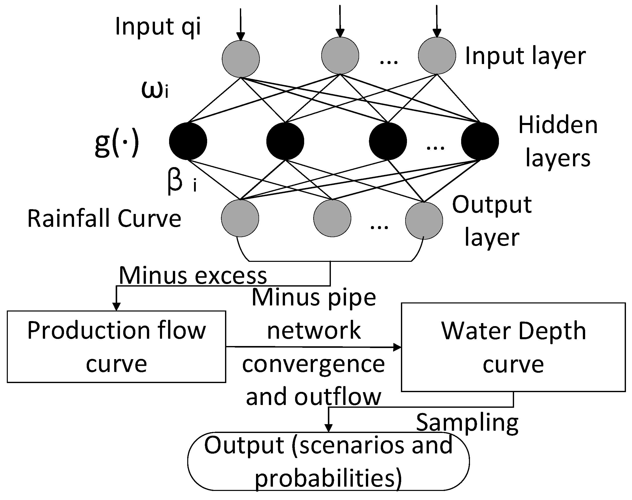
The extreme learning machine (ELM) component comprises three main parts: the input layer, the hidden layer, and the output layer. This structure is depicted in the upper section of Figure 1. Additionally, the lower section of Figure 1 illustrates the process of constructing a mapping model between rainfall intensity and ponding depth using the SWMM model. This model is built based on the rainfall intensity curve generated by the ELM. In summary, the lower part of the figure demonstrates how the SWMM model leverages the rainfall intensity curve produced by the ELM to establish a mapping model for rainfall intensity and water depth.

The model enables the identification of flooding fault scenarios and their associated probabilities in a specific area. It analyzes the rainfall patterns across different regions, distinguishing between pervious and impervious areas, as well as regions with and without depressions [17]. These distinctions account for various forms of rainfall loss, such as evaporation during the rainy season (applicable to both pervious and impervious regions), depression (relevant for impervious areas with depressions), and permeable runoff (pertaining to permeable areas). The runoff is calculated by subtracting these three components from the total rainfall [18]. The mathematical expression is as follows:

I = Q - q_{i} - q_{e} - D

(4)

In Eq (4):

I

denotes rainfall yield; Q denotes total rainfall;

q_{i}

denotes infiltration rainfall;

q_{e}

denotes Evaporation of rainwater (generally not considered); and

D

is the amount of water of low-lying land.

The calculation formula of the infiltration part loss in this area is as follows (the infiltration part is calculated using the Horton infiltration model [19]):

q_{i} = I_{t} * S_{t}

(5)

i_{t} = f_{0} + (f_{1} - f_{0}) e^{- a t}

(6)

In Eq. (5)(6):

i_{t}

is the momentary

t

infiltration rate;

S_{t}

is the area of each permeable zone;

f_{0}

is the final infiltration rate;

f_{1}

is the initial infiltration rate;

a

is the decreasing infiltration rate.

After accounting for the rainfall loss, the model focuses on studying the confluence component to calculate the ponding depth in the relevant area. The confluence component is further divided into two parts: surface confluence and pipeline network confluence. The confluence of the pipeline network refers to the water discharged through the pipeline via the basin outlet. It represents the portion of water flow managed by the drainage system.

The flow rate of the pipeline network is determined by the drainage capacity and drainage time of the network. This capacity indicates the amount of water that can be effectively discharged through the pipeline system within a given period.

The calculation formula is as follows:

Q_{p} = \frac{1}{n} \frac{π d_{r}^{2}}{4} (\frac{d_{r}}{4})^{\frac{2}{3}} {S_{p}}^{\frac{1}{2}} Δ t

(7)

In Eq. (7):

Q_{p}

is the sink flow of the pipe network;

n

is the inner wall of water pipe roughness;

d_{r}

is the pipe diameter;

S_{p}

is the slope of the bottom of the pipe;

Δ t

is the drainage calendar time.

The surface flow process can be effectively modeled by considering the catchment as a nonlinear reservoir. In this modeling approach, the catchment area is taken into account, and the flow rate is used as an input to the model. By analyzing the relationship between the outflow rate at the basin outlet and the water depth, a nonlinear function describing this relationship can be derived. The nonlinear reservoir model is calculated as follows:

\frac{d V}{d t} = S \frac{d d}{d t} = S i - Q_{c}

(8)

Q_{c} = W_{f l} \frac{1.49}{n} (d - d_{p})^{\frac{5}{3}} S_{l}^{\frac{1}{2}}

(9)

In Eq. (8)(9):

V

is the water volume in catchment area

V = s * d

;

d

is the nodal corresponding water depth;

S

is the area of the catchment area;

i

is the produced flow calculated by the previous part;

Q_{c}

is the outflow;

W_{f l}

is the diffuse width of the catchment area [20] means the distance that the fluid expands horizontally on the bed in a region with uneven topography;

n

is the surface Manning roughness coefficient whose value differs significantly between permeable and impermeable areas;

d_{p}

is the surface stagnant water depth whose value was obtained by analyzing the land elevation data; and

S_{l}

is the slope of the catchment area. Combining equations (8) and (9) can obtain

d

and

Q_{c}

. After considering the prediction error (error calculation is explained in Section 3.2) to obtain the predicted ponding depth of the corresponding node of the power facility. When the predicted water level is greater than or equal to the height of the substation, it is considered that a risk event occurs.

The initial scenario of water immersion failure is generated using a non-sequential Monte Carlo sampling method, which allows for the generation of diverse and representative scenarios. This process involves randomly sampling from a range of possible inputs to obtain a set of initial fault scenarios. The corresponding probabilities of these scenarios are then calculated. The generation process for the initial fault scenarios in the power system is presented in Table 1.

3.2. Generate the initial set of scenes

Based on the previous section's introduction, a water depth curve over time can be calculated for a specific area based on the predicted values of the rainfall intensity curve. However, it is important to consider that there may be some errors in the prediction of rainfall intensity. These errors can arise due to the inherent randomness in historical data, potentially leading to data quality issues. In this paper, it is assumed that the fluctuation between the actual rainfall intensity and the predicted value follows a normal distribution. The amplitude of the error fluctuation curve is considered to conform to a 3σ normal distribution, with the expected value corresponding to the intensity of the predicted rainfall at that moment. The expression of the error value is shown in Eq (10).

f (x; μ; δ) = \frac{1}{\sqrt{2 π} δ} * e x p (- \frac{{(x - μ)}^{2}}{2 σ^{2}})

(10)

In Eq (10),

x

is the prediction error value,

μ

is the predicted rainfall intensity value, and

δ

is the mathematical variance. A normal random number, also known as a Gaussian random number, is a number generated from a normal distribution. In a normal distribution, the probability of occurrence is highest around the mean (expectation) value and decreases as the number deviates from the mean.

To determine the operational status of the substation, suppose there are

n

substations in a power grid, and the state probability characteristics of each substation are described by a random number that obeys the 0-1 distribution [21], and each substation has only two states of normal and fault, normal corresponds to 1, fault corresponds to 0, and whether different substations are faulty is independent of each other. The substation number is denoted as

k

S_{k}

indicating the operating state of the substation

k

, and the grid operating state (denoted as

S

) is composed of the states of each substation in the grid. Therefore, the operating state of the grid can be expressed as

S = (S_{1}, S_{2}, \dots {, S}_{n})

, that means the initial fault scenario of the power facility is obtained.

The final water depth value is obtained by taking into account both the calculation method and the prediction error of the water accumulation height, as proposed in the previous section. By comparing this final water depth value with the height of the substation, the operational status of the substation can be determined.

This approach ensures a comprehensive evaluation of the water accumulation height, considering both the calculated value and the potential prediction errors. The height of multiple substations in the order of

H_{1}

H_{2}

\dots, H_{n}

. Determine the substation status according to the following equation.

S_{k} = \{\begin{matrix} 0 d_{t} \geq H_{k} \\ 1 d_{t} ＜ H_{k} \end{matrix}

(11)

In Eq (11):

S_{k}

is the state of the substation

k

H_{k}

is the state of the substation

k

, and

d_{t}

represents the ponding depth at the moment

t

. The sampling process is shown in Figure.2.

Figure 2. Sampling process.

3.3. Building typical scenario sets

Once the initial library of failure scenarios is generated, the scenarios whose occurrence probability is significantly lower than the others are ignored according to statistical principles. The resulting typical scenario set fully represents the possible fault scenarios in reality, and provides more scientific guidance for the safe and stable operation of the power system. Through the setting of typical scenarios, more specific and targeted preventive measures can be implemented for different fault scenarios, effectively reducing losses caused by risk events. In addition, the typical scene set has important reference value for the formulation of emergency plans. By considering different failure scenarios, corresponding contingency plans can be developed in advance, ensuring the proper configuration of personnel and equipment to respond quickly and efficiently in the event of a failure.

In summary, the generation of a typical scenario set offers practical benefits for power system operations. It allows for tailored preventive measures, minimizes losses resulting from risk events, and aids in the formulation of proactive emergency plans. This comprehensive approach enhances the overall resilience and reliability of the power system.

4. Stochastic Power Flow Calculation Considering Load Uncertainty

4.1. Calculation of semi-invariance of each order in a typical scenario

Define the typical outage scenarios of each power facility generated above as

T_{j}

.The probability density function

f_{j} (x)

and cumulative distribution function

F_{j} (x)

of the power system state quantity

x

considering the load uncertainty under the scenario a can be obtained by semi-invariant method and the Gram-Charlier series expansion method.

Prior to calculating the semi-invariants of each order for each random variable, it is essential to conduct deterministic power flow calculations. These calculations are performed to determine the reference operating point of the power grid. On this basis, the bus voltage state variable

Δ X

and the branch power flow state variable

Δ Z

can be further obtained according to the random distribution of the load, and the Jacobian matrix

J_{0}

(Power System Jacobian Matrix) and sensitivity matrix

S_{0}

(Sensitivity Matrix) can be calculated .The nodal and branch equations of the power system are expressed as shown in Eq. (12) and Eq. (13) after carrying out Taylor series expansion at the base operating point and neglecting the higher terms of 2 or more times.

W = W_{0} + Δ W = f (X) = f (X_{0} + Δ X) \approx f (X_{0}) + J_{0} * Δ X

(12)

Z = Z_{0} + Δ Z = g (X) = g (X_{0} + Δ X) \approx g (X_{0}) + G_{0} * Δ X

(13)

In Eq(12) and Eq(13),

W

is bus injection variable;

X

is bus state variables;

Z

is branch state variables;

J_{0} = {\frac{\partial f (X)}{\partial X}|}_{X = X_{0}}

G_{0} = {\frac{\partial g (X)}{\partial X}|}_{X = X_{0}}

The following equation conditions are satisfied at the reference operating point of the power grid.

\{\begin{matrix} W_{0} = f (X_{0}) \\ Z_{0} = g (X_{0}) \end{matrix}

(14)

Then the linearization equation for the random perturbation

Δ W

at the reference operating point of the power grid can be obtained. The linearized equation is shown in equation (15):

\{\begin{matrix} Δ X = J_{0}^{(- 1)} Δ W = S_{0} Δ W \\ Δ Z = G_{0} S_{0} Δ W = T_{0} Δ W \end{matrix}

(15)

According to the homogeneity and additivity of the semi-invariant [22] and the relationship between the power system bus injection quantity and the state quantity in formula (15), half of the system state quantity can be obtained according to the semi-invariant of the bus injection variable invariant.

4.2. Gram-Charlier series expansion method

Based on the semi-invariants of each order for each random variable, the probability density function and cumulative distribution function of each random variable can be determined using the Gram-Charlier series expansion method. The Gram-Charlier series expansion method allows for expanding the distribution function of a random variable into a series consisting of derivatives of each order of the normal random variable. The coefficients of the series can be expressed as the semi-invariants of each order of the random variable [23]

g_{v} = \frac{γ_{v}}{δ^{v}} = \frac{γ_{v}}{γ_{2}^{v / 2}}

(16)

In Eq. (16):

γ_{v}

is called the

v

order normalized semi-invariant and is also the coefficient in each expansion of the Gram-Charlier series;

δ

is the standard deviation.

Let

F (x)

and

f (x)

be the cumulative distribution function and the probability density function of the standardized random variable

x

, respectively, the

f (x)

is the derivative of

F (x)

. The Gram-Charlier series expansions of

F (x)

and

f (x)

are of the following form [20]:

F (x) = \int_{x}^{\infty} φ (x) d x + φ (x) [\frac{g_{3}}{3!} H_{2} (x) + \frac{g_{4}}{4!} H_{3} (x) + \frac{g_{5}}{5!} H_{4} (x) + . . .]

(17)

f (x) = φ (x) [1 + \frac{g_{3}}{3!} H_{3} (x) + \frac{g_{4}}{4!} H_{4} (x) + \frac{g_{5}}{5!} H_{5} (x) + . . .]

(18)

In Eq. (17)(18):

φ (x)

is the probability density function of the standard normal distribution;

H_{v} (x)

denotes the Hermite polynomial of

v

order Hermite polynomials are a set of orthogonal polynomials, which are usually used to deal with problems related to quantum mechanics, mathematical physics and probability theory.

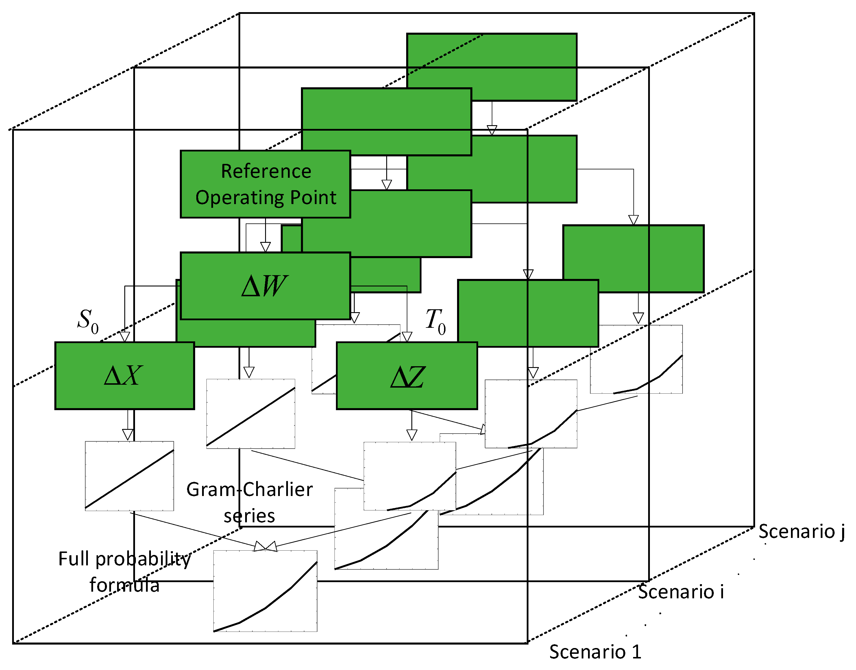
In summary, based on the semi-invariant and Gram-Charlier series expansion stochastic power flow algorithm process is shown in Figure 3:

In Figure 7, after the reference operating point is calculated, the node injection variable

Δ W

is obtained according to the load fluctuation, the sensitivity matrix

S_{0}

and the transfer matrix

T_{0}

are obtained after constructing the Jacobian matrix, and then the probability density function and cumulative distribution function of different initial fault scenarios are obtained. Next, the corresponding results for each typical set of scenes and synthetic scenes are calculated using the total probability formula. A more comprehensive understanding of system performance can be obtained by employing a fully probabilistic formulation and considering the collective impact of multiple scenarios.

\{\begin{matrix} f (x) = \sum_{j = 1}^{n} p_{j} f_{j} (x) \\ F (x) = \sum_{j = 1}^{n} p_{j} F_{j} (x) \end{matrix}

(19)

In Eq. (19):

p_{j}

is the probability of occurrence of typical scene

j

;

f_{j} (x)

and

F_{j} (x)

are the calculation results of the probability distribution of variable

x

in scene

j

respectively.

5. Particle swarm algorithm based decision model for load curtailment optimization

5.1. Optimal load curtailment model

During the operation of power systems, various risk events can occur as a result of power facility failures and load fluctuations. In order to address this challenge, this paper presents a nodal load curtailment optimization model based on stochastic power flow. The proposed model ensures the power balance of the system while preventing branch power flows from exceeding their limits. By optimizing the load curtailment at each bus, the model aims to minimize the risk of power system failures and maintain stable operations. The objective function of the optimization model is formulated as the product of the probability of occurrence under a typical scenario set and the minimum expected reduction in bus load under different scenario sets. Mathematically, the bus load curtailment optimization model can be represented as follows:

E_{a l l} = \min \sum_{s e}^{N S} P_{s e} \sum_{i}^{N D} α C_{i}

(20)

In Eq. (20):

E_{a l l}

is the expected sum of load curtailment for all typical scenario sets;

N S

is the number of typical scenario sets obtained by statistical methods;

P_{s e}

is the probability of occurrence of any typical scenario set;

α

is a weighting factor used to indicate the types of different buses;

C_{i}

is the load curtailment on bus

i

;

N D

is the set of load buses.

Constraints:

0 \leq C_{i} \leq P D_{i} (i \in N D)

(21)

The physical meaning of Eq. (21) is that the amount of curtailment of load on bus

i

cannot be greater than the rated load on bus

i

F (|T_{k} (S)| \geq T_{k}^{m a x}) \leq 0.05

(22)

In Eq. (22)

T_{k}^{m a x}

is the value of the volt-amperes tidal current withstood on line

k

T_{k} (S)

is the rated transmitted power on line

k

F (|T_{k} (S)|)

is the tidal current crossing probability of each branch.

5.2. Load Importance Level

According to the literature [24], power system emergencies can lead to losses in various load categories. These losses can be classified as social, economic, and political losses. The qualitative relationship between each type of loss can be obtained from the literature as follows:

Social loss: Social loss primarily revolves around ensuring life safety and maintaining public order during power system emergencies. It considers the impact on individuals, communities, and public welfare.
Economic loss: Economic loss encompasses the loss of power supply and equipment damage caused by power system emergencies. It takes into account the financial impact on businesses, industries, and the overall economy.
Political loss: Political loss focuses on the negative consequences of load curtailment on government department operations and public administration during power system emergencies.

The analysis using AHP [25] (Analytic Hierarchy Process) and ANP [26] (Analytic Hierarchy Process) allows for a comprehensive assessment of different load buses, considering their respective social, economic, and political importance. The results of the analysis, as shown in Table 2.

5.3. Particle swarm algorithm based solution process

Particle Swarm Optimization (PSO) is an optimization algorithm inspired by the foraging behavior of birds. It mimics the collective behavior of individuals in a flock to efficiently search for the optimal solution to a given problem. In PSO, candidate solutions are represented as a group of particles, with each particle representing a potential solution in the search space. These particles iteratively update their positions and velocities based on individual and group experiences, aiming to converge towards the optimal solution.

The algorithm involves several key factors, including acceleration factors

c_{1}

and

c_{2}

, and the inertia factor

ω

These factors influence the speed at which particles move towards their individual optimal positions and the global optimal position, balancing exploration and exploitation. In this paper, an improved particle swarm algorithm is employed to calculate the objective function. To ensure the feasibility of the solutions, a constraint function is added to the original objective function as a penalty function. This penalty function guides the iterative process to approach the feasible region of the solution space, encouraging the particles to converge towards viable solutions. By integrating these enhancements into the particle swarm optimization framework, the algorithm in this paper can effectively search for optimal solutions while satisfying the specified constraints. The solution formula of the penalty function is explained as formula (23).

F (x, M) = f (x) + M p (x)

(23)

In Eq. (23):

f (x)

is the objective function;

M p (x)

is the penalty term. The penalty factor M is a sufficiently large real number, and the optimal solution of

F (x, M)

is close to the optimal solution of the constrained problem.

6. Example analysis

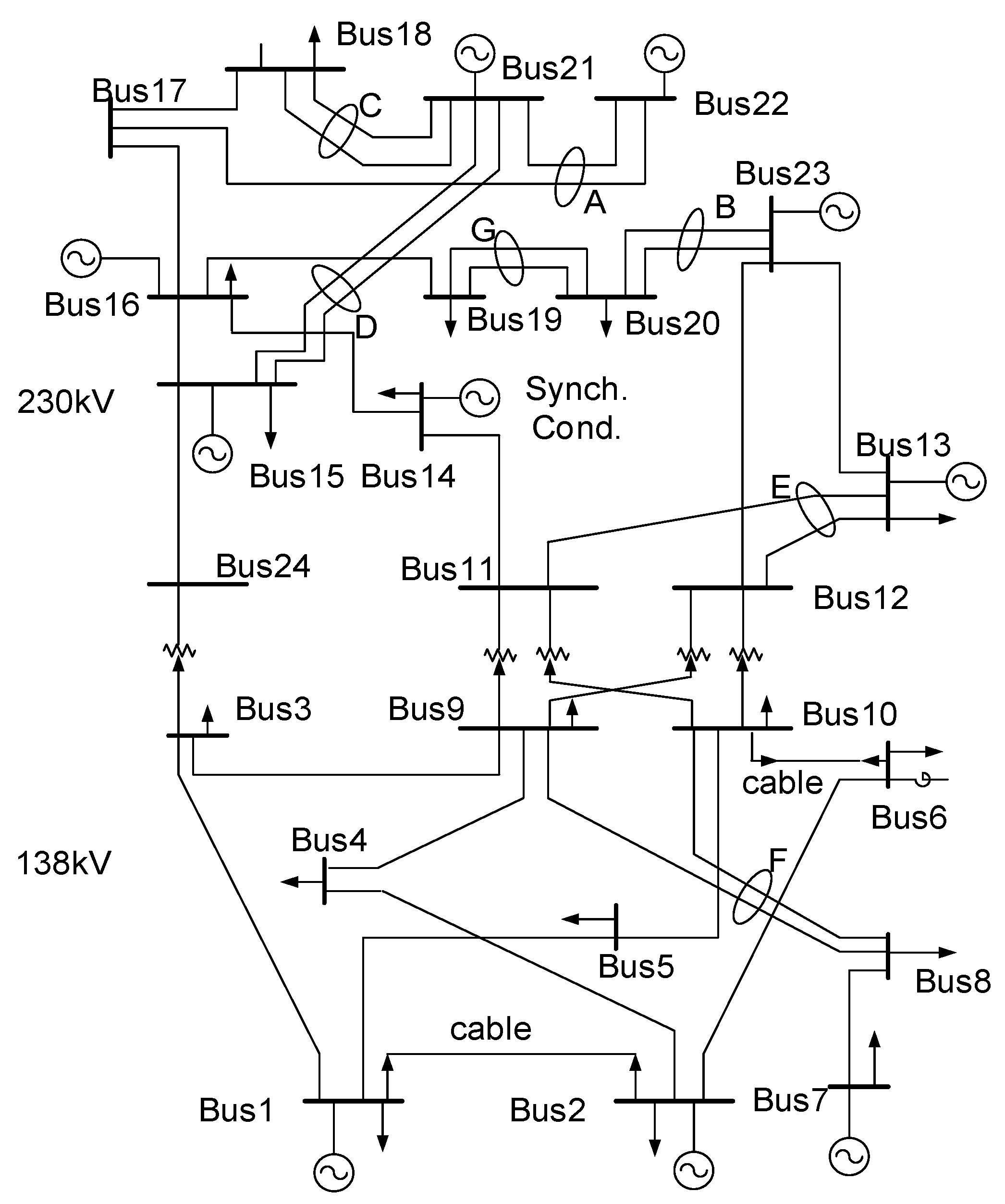
In this paper, the IEEE 24-bus system is used as an example for simulation purposes. The buses in the system are categorized into three classes: buses 1-8 are classified as Class I loads with a weight factor of 0.5, buses 9-16 are designated as Class II loads with a weight factor of 0.3, and buses 17-24 are categorized as Class III loads with a weight factor of 0.2. To model load fluctuations, numerous relevant literature sources indicate that these fluctuations follow a normal distribution pattern. Therefore, it is assumed in this study that the load fluctuations at each bus conform to a normal distribution. The expected value of the load fluctuation is set as the rated value of the respective bus load, and the standard deviation is assumed to be 20% of the average value.

The network topology of the power system is illustrated in Figure 4.

6.1. Typical scenario generation

6.1.1. Outage scenario generation model

Table 3 presents the relevant data necessary for the fault scenario generation model of power facilities proposed in this study. This dataset includes essential information required for the analysis and assessment of power system faults.

6.1.2. Rainfall and water distribution

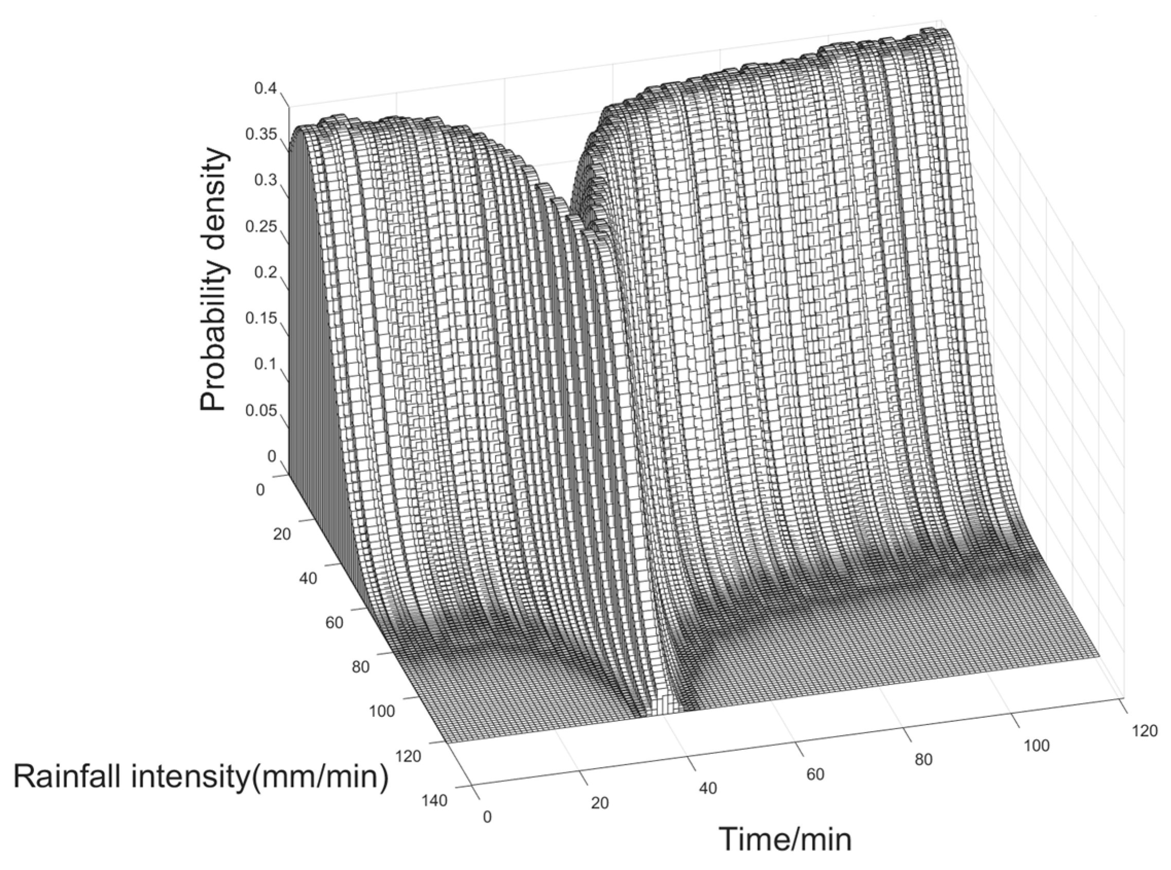
Assuming that the rainfall intensity follows a standard normal distribution, Figure 5 presents a three-dimensional plot showcasing the relationship between time, rainfall intensity, and the corresponding probability density. In the plot, the X-axis represents time in minutes, the Y-axis represents the instantaneous rainfall intensity in millimeters per minute (mm/min), and the Z-axis represents the probability density associated with the instantaneous rainfall intensity at a given time.

Figure 5 depicts the fluctuation of rainfall intensity within a specific range over time. It is observed that the rainfall intensity varies within certain bounds, exhibiting temporal variations. The probability density initially increases and then decreases as time elapses. As time advances, the probability density distribution reflects the changing likelihood of different rainfall intensity values. Moreover, it is apparent from the plot that when the rainfall intensity is large, the corresponding probability density tends to be smaller. This suggests that extreme rainfall events, characterized by higher intensities, occur with lower probabilities compared to moderate or lower intensity rainfall.

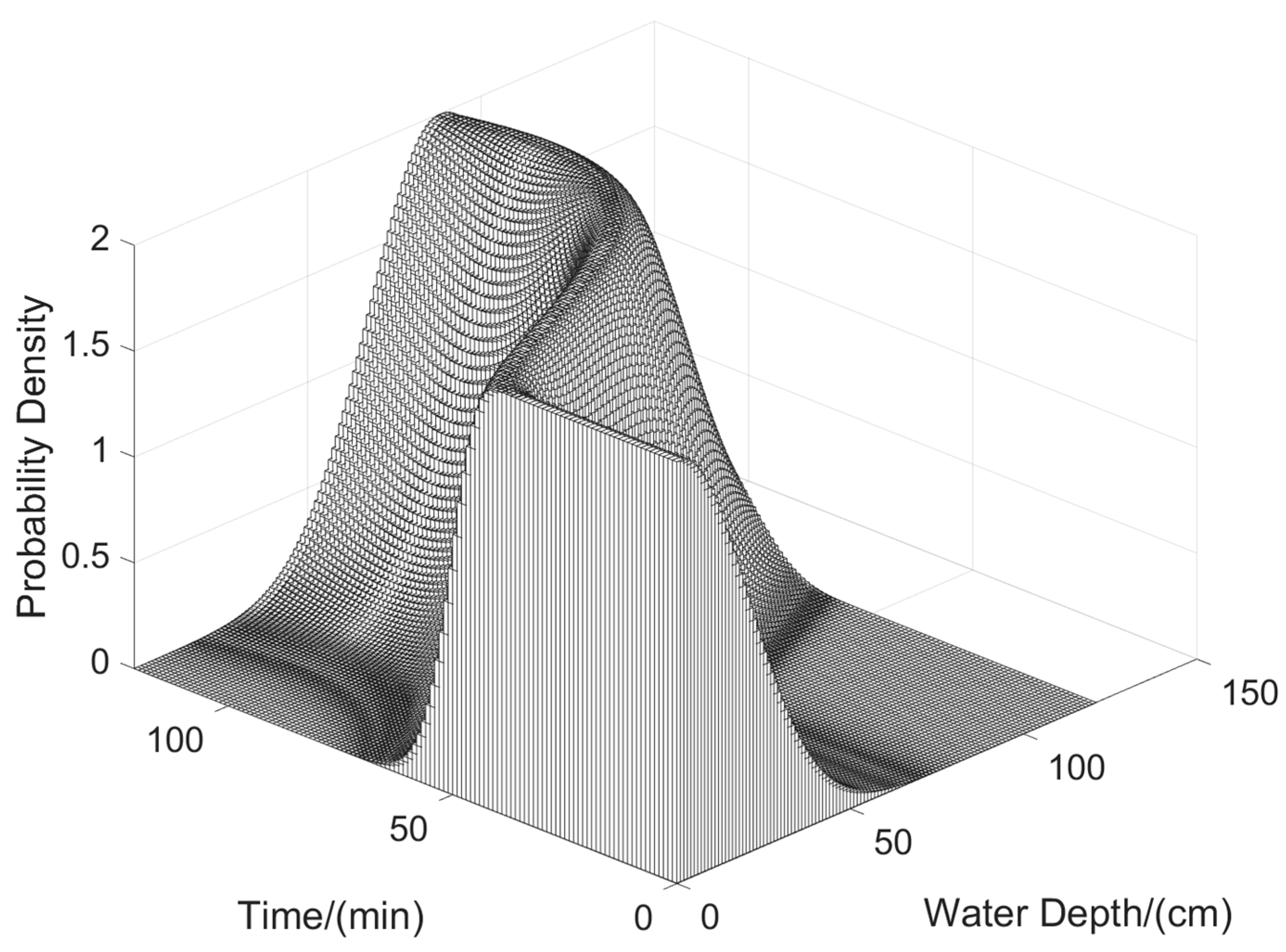
The observations derived from Figure 6 offer valuable information about the probabilistic characteristics of water depth over time. It is apparent that the probability density decreases as water depth increases during the first half of the time period. Moreover, in the second half of the time, the rate at which water depth increases, corresponding to higher probability density, gradually slows down. This suggests that as water depth reaches higher levels, the likelihood of further significant increases diminishes.

6.1.3. Scene library generation and reduction

After obtaining the distribution of rainfall intensity, the power system outage scenarios and their respective probabilities are determined using Monte Carlo sampling, as illustrated in Figure 7. The sampling is performed 10,000 times to capture a comprehensive range of possible scenarios. Within the considered power system, there are five substations with different heights: 0.95m, 0.9m, 0.85m, 0.8m, and 0.75m

Figure 7. Failure Scenarios and their corresponding probability histograms.

The bar chart presented in Figure 7 displays the results after applying statistical theory to discard low probability events. In this chart, (a), (b), and (c) represent the probabilities of occurrence for the same initial failure scenario under different conditions. The typical scenarios depicted in the bar chart are differentiated based on the number of faults occurring in the substations. Each bar represents a specific scenario, and its height corresponds to the probability of that scenario occurring. This approach ensures that the subsequent analysis and decision-making processes are based on typical scenarios that possess higher probabilities of occurrence.

6.2. Curtailment of load simulation results

To validate the efficacy of the proposed method, the benchmark value is defined as the power capacity that each branch can withstand under normal operating conditions. In this context, the power of 1.2 times the normal operating level is set as the limit for overloading. Table 4 provides the values of the power capacity for each branch under normal operating conditions.

Table 5 lists the total grid load reduction for each typical scenario group. It shows the cumulative load shedding taking into account power system load fluctuations under various conditions. It is found through analysis that the total load shedding of all buses in the power system increases with the number of substation faults. This indicates that as the number of substation failures increases, more loads need to be shed to maintain power system stability and avoid overloading.

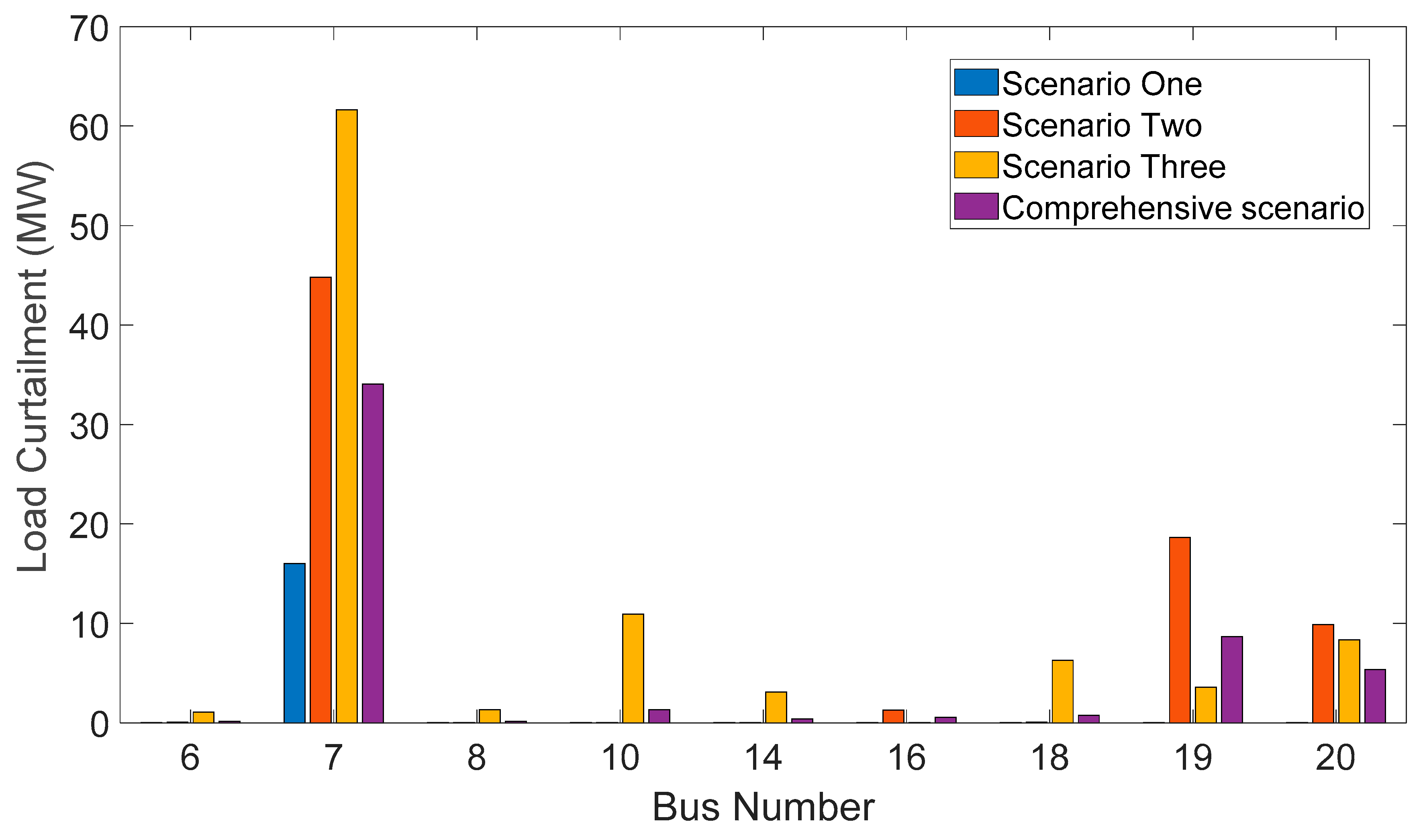
Figure 8 illustrates the load curtailment at the main buses for each typical scenario set and the comprehensive scenario. It is important to note that the load curtailment amounts at other buses, which are not depicted in the figure, are considerably smaller compared to the buses displayed. The focus of Figure 8 is on showcasing the load curtailment levels at the main buses that are most significantly impacted by the identified scenarios. These buses are typically the ones experiencing the highest load curtailment requirements and therefore require particular attention in terms of load management strategies and contingency planning.

6.3. Simulation results of branch power flow violation

Branches 7, 14, 15, 16, and 17 are designated as fault setting points in the analysis. It is important to note that when the load at bus 24 is zero, the power flow on branch 27 (between bus 15 and bus 24) is considered to be zero in the event of a failure on the branch connecting bus 3 and 24.

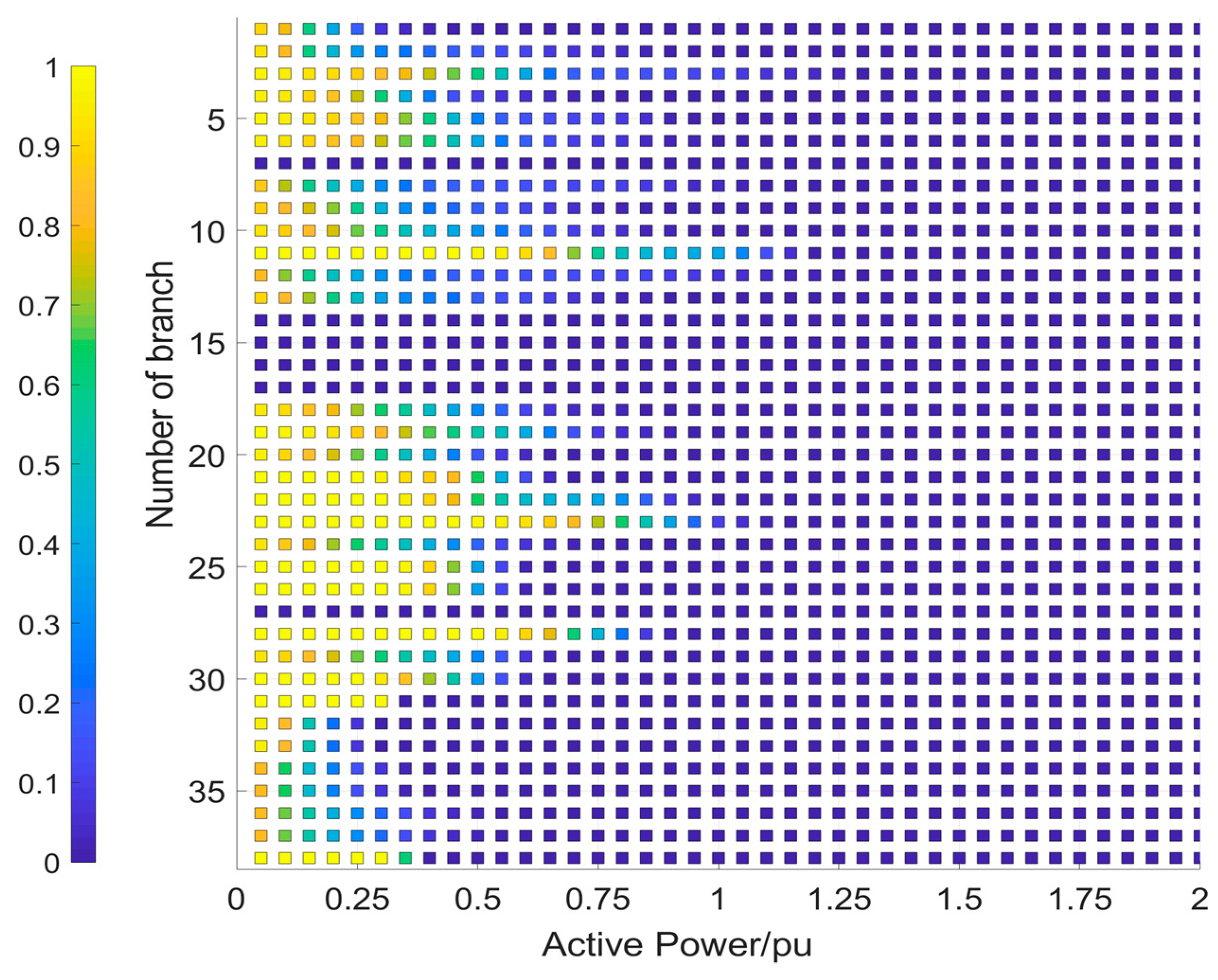
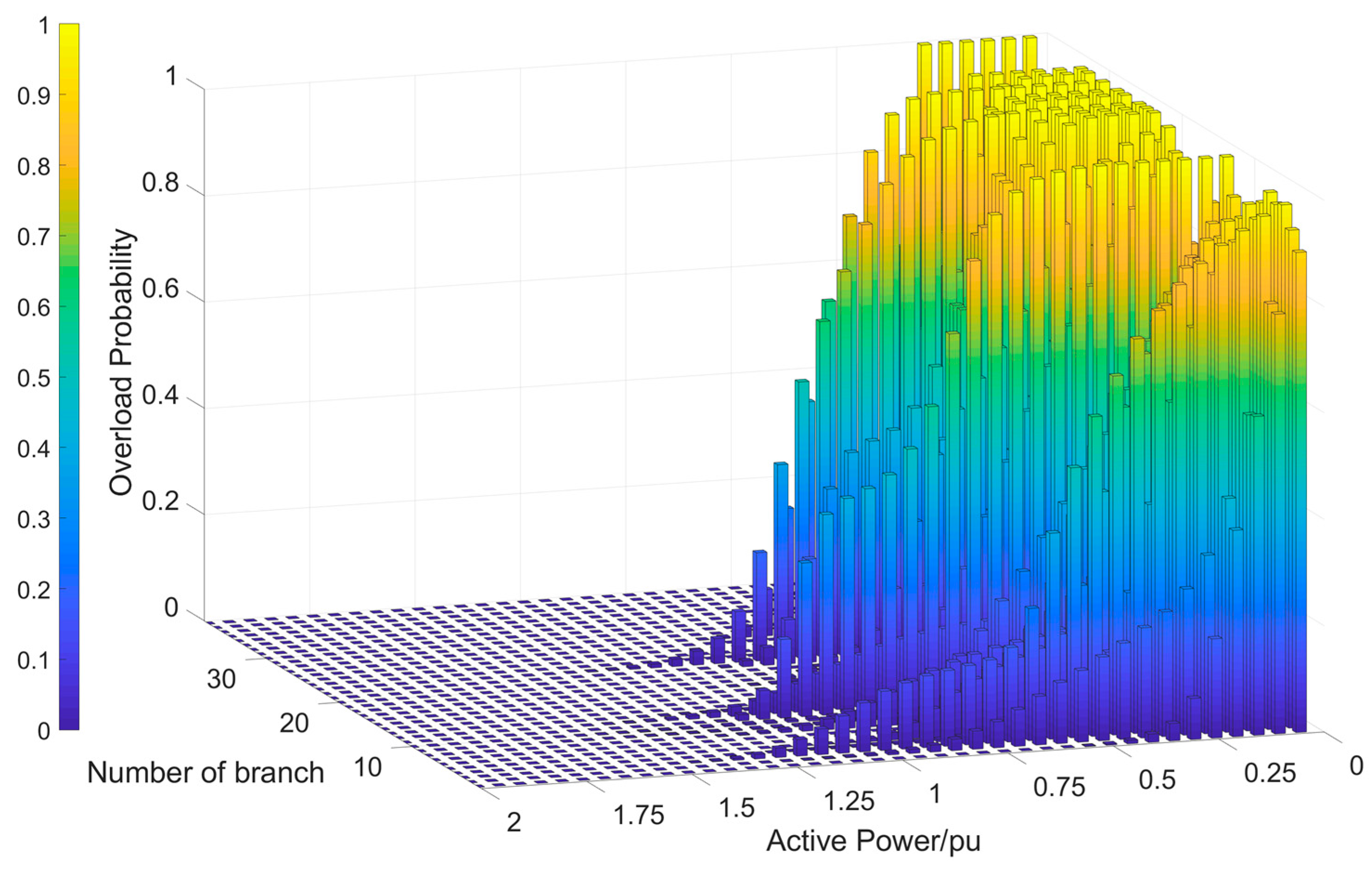
By analyzing Figure 9 and Figure 10, it is evident that branch 3 has an overreach probability of 3.56% at a power flow level of 1.2 pu, while branch 23 has a crossing limit probability of 0.52% at the same power flow level. It is worth noting that the overload probability of each branch in the comprehensive scenario remains below 5%. That demonstrates the model's effectiveness in identifying potential issues and evaluating the system's ability to maintain stability under varying conditions. This validation of the proposed model's performance highlights its value in decision-making processes related to load curtailment strategies and risk mitigation measures.

7. Conclusions

This paper employs the IEEE 24-bus system as a case study to validate the effectiveness of the proposed method. It supplements the existing power system risk assessment framework by incorporating the analysis of extreme rainfall weather conditions. The main features of this method can be summarized as follows:

The proposed approach involves determining the rainfall curve and the corresponding water accumulation curve through the combined use of the SWMM model and the extreme learning machine. To assess the probabilities of different initial fault scenarios, the Monte Carlo sampling method is applied. Using statistical theory, the initial fault scenarios are refined, resulting in the identification of typical scenario sets. These sets comprise specific fault scenarios with their corresponding probabilities.
The branch power flow overload probability of each initial scenario within a single typical scenario set is calculated using the semi-invariant and Gram-Charlier series expansion methods. By applying the full probability formula, the power grid overload probability is obtained for each typical scenario set. This calculation takes into account the probabilities of branch power flow overloads in the specific scenarios within the set. With the power grid overload probabilities determined for each typical scenario set, it becomes possible to calculate the power grid overload probability in the comprehensive scenario. This calculation involves aggregating the probabilities from all the typical scenario sets to provide an overall assessment of the likelihood of power grid transgressions.
In the optimal load curtailment model, the branch active power violation probability is incorporated as a constraint. This ensures that the power flow in each branch remains within the specified limits. To solve the constrained optimization problem, the particle swarm optimization (PSO) algorithm is employed. To handle the constraints, a penalty function approach is adopted, transforming the constrained optimization problem into an unconstrained one. This technique helps to speed up the solution process by converting the problem into a form that is more amenable to optimization algorithms like PSO.

Funding

This research was funded by the Science and Technology Project of State Grid of Zhejiang Electric Power Company, Ltd. (Project Number: 2022-KJLH-BC-012)

Conflicts of Interest

The authors declare that there is no conflict of interest.

References

Z.X, Yi; Z.L, Chen; K, Yin; L.C, Wang; K, Wang. Sensing as the key to the safety and sustainability of new energy storage devices. Protection and Control of Modern Power Systems, 2023, 8, 27.
L.C, Wang.; L.C, Xie; Y, Yang.; Y.B, Zhang. Distributed online voltage control with fast PV power fluctuations and imperfect communication. IEEE Transactions on Smart Grid (2023). [CrossRef]
S.Z, Xu; J.G, Gong. Lightning protection measures and zoning lightning protection for transmission lines in medium and heavy ice areas. Electric porcelain lightning arrester,2021, (4): 47-54.
C.Z, Xie; J.F, Bai; H.B, Wang. Risk assessment of transmission line over-icing disaster considering multiple factors based on evolutionary strategy-projection tracing algorithm. Power System Automation, 2013, 37(10): 92-97.
J.J, Song. Time-varying outage model for overhead transmission lines under severe disasters (Hangzhou: Zhejiang University,2013.
Y, Chen. Research on Risk Assessment and Control of Wenzhou Power System Considering Extreme Weather. Hangzhou: Zhejiang University,2022.
W, Riley; E.C, Sanchez; Ted. KA, Brekken. Toward Models of Impact and Recovery of the US Western Grid from Earthquake Events. Energies 15.24 (2022): 9275. [CrossRef]
R. A, Swief; T. S, Abdel-Salam; N. H. El-Amary. Photovoltaic and wind turbine integration applying cuckoo search for probabilistic reliable optimal placement. Energies 11.1 (2018): 139. [CrossRef]
X.Y, Deng; J.H, He; P, Zhang. A novel probabilistic optimal power flow method to handle large fluctuations of stochastic variables. Energies 10.10 (2017): 1623. [CrossRef]
X, Ye; Y.F, Wang; Multipoint linearized probabilistic power flow calculation with correlation of random variables Journal of Power Systems and their Automation:1-9[2023-05-16].
H.R, Lian, B.R, Zhou; Stochastic power flow resolution algorithm based on scenario partitioning. Power Grid Technology,2017,41(10):3153-3160.
P, Wei; J.K, Liu; Stochastic power flow algorithm based on semi-invariant and Gram-Charlier level expansion method. Power Engineering Technology,2017,36(01):34-38.
C, Li; Y, Zeng; An optimal dispatching method for power systems accounting for operational risks. Journal of Power Systems and their Automation,2016,28(06):73-79.
Y. Jia; W .X, Li. Penalty function improved particle swarm algorithm for optimal configuration of scenery storage system. Journal of Solar Energy,2019,40(07):2071-2077.
Q, Li. SWMM-based reliability analysis of urban stormwater pipe network and multi-objective reconstruction optimization research Dalian: Dalian University of Technology,2016.
L, Zhou; Z.X, Huang. Extreme learning machine for short-term power system load forecasting. Electronic World,2021(08):33-34.
S.S, Wang. Research on the application of production and convergence forecasting models in early warning systems Nanchang: Nanchang University,2019.
X. F, Rui. Discovery and development of the production flow model. Advances in Water Resources and Hydropower Science and Technology2013 (01), 1-6+26.
D. Q, Zhao; J.N Chen, Study on the influence of sub-catchment delineation on SWMM simulation results. Environmental Protection,2008(08):56-59.
X. T, Zeng. Study on the optimization model of stormwater pipe network based on NSGA-II algorithm Research. Chengdu: Southwest Jiao tong University,2021.
L, Xu. Power system voltage collapse risk assessment Chongqing: Chongqing University,2009.
W.T, Zhang; L.X, Fan. Wind power penetration power limit calculation based on DC probabilistic currents. Jiangsu Electrical Engineering,2014,33(04):1-4.
J.H, Fan; N, Xu. Fault recovery strategy for power distribution systems with distributed scenic power. Jiangsu Electrical Engineering,2014,33(01):1-4+8.
C.Y, Bian; X. Y, Fang. Site selection model of electric power emergency material storage considering load level. Journal of Power Systems and their Automation, 2017,29(01):78-83.
W.Q, Kang. A security risk assessment method for power monitoring network based on improved AHP algorithm. Automation and Instrumentation:2022(10):171-174.
26. X.J, Wang; Y, Huang. Comprehensive evaluation and type selection of energy storage based on hierarchical analysis method Zhejiang Electric Power,2022,41(11):1-8.
Subcommittee, P. M. "IEEE reliability test system." IEEE Transactions on power apparatus and systems 6 (1979): 2047-2054.

Figure 1. The generation process of power facility fault scenarios.

Figure 3. Flow chart of stochastic power flow algorithm.

Figure 4. Diagram of IEEE 24-bus system topology.

Figure 5. Three-dimensional plot of time, rainfall intensity and probability density.

Figure 6. Three-dimensional plot of time, water depth and probability density.

Figure 8. Bus Load curtailment in each scenario.

Figure 9. The overload probability of each branch in the comprehensive scenario（2D）.

Figure 10. The overload probability of each branch in the comprehensive scenario（3D）.

Table 1. Failure scenario generation process.

Algorithm: Electric utility failure scenario generation process
Input: past storm curve data $X_{i}$ activation function $g (\cdot)$ , number of hidden layer neurons $K$ ; Output: probability of failure of electrical facilities
1:	Import a rainfall dataset as input, noted as storm curve data $X_{i}$ ;
2:	Data preprocessing: processing of the desired output into a row vector, where each element of the vector represents a category, and calculation of the desired output matrix $y_{h}$ ;
3:	Set the activation function $g (\cdot)$ , the number of hidden layer neurons $K$ , and randomly initialize the weight matrix $W$ and the bias vector $b$ between the input layer and the hidden layer,where the weights are randomly generated between [-1,1] and the connection bias is randomly generated between [0,1];
4:	Calculate the hidden layer output matrix according to Eq (1), where $X$ is the matrix with each element being past storm curve data
5:	Calculate the output layer weight matrix according to Eq (2);
6:	Calculation of the output prediction data and visualization of the rainfall curve according to Eq (3);
7:	Calculate the amount of infiltration $q_{i}$ according to Eq (5) and Eq (6);
8:	Enter the puddle storage and evaporation volumes and calculate the production flow according to Eq (4);
9:	Calculate the pipe network sink flow rate $Q_{p}$ according to Eq (7);
10:	Calculate the variation curve of the ponded water level with time for a given precipitation intensity profile for the power facility according to Eq (8) and Eq (9).

Table 2. Load importance.

Class	Types
Class I	Government buildings, subway stations, airports, etc.
Class II	Commercial buildings, playgrounds, small factories, etc.
Class III	Residential areas, etc.

Table 3. Data required for outage mode.

Heading	Value in the model	Heading	Value in the model
Catchment area/m²	15000	Pipe Manning Roughness	0.01
Flood width /m	140	Pipe diameter/m	0.3
Catchment slope /%	0.2	Pipe bottom slope	0.2
Permeable Area Ratio/%	20	Maximum permeability/(m·min-1)	1.2
Manning roughness of impervious area	0.013	Minimum permeability/(m·min-1)	0.06
Manning roughness of permeable area	0.1	Permeability attenuation coefficient (min-1)	0.1

Table 4. Normal operating power for each branch of the IEEE 24-bus system.

Branch	MVA	Branch	MVA	Branch	MVA	Branch	MVA
1-2	175	7-8	175	12-23	500	17-22	500
1-3	175	8-9	175	13-23	500	18-21	500
1-5	175	8-10	175	14-16	500	18-21	500
2-4	175	9-11	400	15-16	500	19-20	500
2-6	175	9-12	400	15-21	500	19-20	500
3-9	175	10-11	400	15-21	500	20-23	500
3-24	400	10-12	400	15-24	500	20-23	500
4-9	175	11-13	500	16-17	500	21-22	500
5-10	175	11-14	500	16-19	500
6-10	175	12-13	500	17-18	500

Table 5. Total load curtailment in each typical scenario.

Scenarios	Total load curtailment (MVA)
Scenarios One	16.06
Scenarios Two	74.83
Scenarios Three	97.32
Comprehensive scenes	51.52

Disclaimer/Publisher’s Note: The statements, opinions and data contained in all publications are solely those of the individual author(s) and contributor(s) and not of MDPI and/or the editor(s). MDPI and/or the editor(s) disclaim responsibility for any injury to people or property resulting from any ideas, methods, instructions or products referred to in the content.

© 2023 by the authors. Licensee MDPI, Basel, Switzerland. This article is an open access article distributed under the terms and conditions of the Creative Commons Attribution (CC BY) license (http://creativecommons.org/licenses/by/4.0/).

Copyright: This open access article is published under a Creative Commons CC BY 4.0 license, which permit the free download, distribution, and reuse, provided that the author and preprint are cited in any reuse.

MDPI Initiatives

Important Links

Choose an area of interest and we will send you notifications of new preprints at your preferred frequency.

Disclaimer

Risk Assessment of Power Supply Security Considering Electricity Facility Outages in Extreme Precipitation Scenarios

Abstract

1. Introduction

2. Risk analysis framework considering waterlogged failures

3. Generation of typical fault scenarios for power facilities under extreme rainfall

3.1. Power Facility Failure Model

3.2. Generate the initial set of scenes

3.3. Building typical scenario sets

4. Stochastic Power Flow Calculation Considering Load Uncertainty

4.1. Calculation of semi-invariance of each order in a typical scenario

4.2. Gram-Charlier series expansion method

5. Particle swarm algorithm based decision model for load curtailment optimization

5.1. Optimal load curtailment model

5.2. Load Importance Level

5.3. Particle swarm algorithm based solution process

6. Example analysis

6.1. Typical scenario generation

6.1.1. Outage scenario generation model

6.1.2. Rainfall and water distribution

6.1.3. Scene library generation and reduction

6.2. Curtailment of load simulation results

6.3. Simulation results of branch power flow violation

7. Conclusions

Funding

Conflicts of Interest

References

MDPI Initiatives

Important Links

Subscribe