1. Introduction
There are several types of rotative encoders, each with its own advantages and disadvantages. Here are some of them:
1. Optical encoders: Some of these encoders use a disk with slots that interrupts the light emitted by an LED or laser to generate digital signals that indicate position. Optical encoders have high resolution, are precise, and can be used in high-speed applications. However, they are susceptible to electromagnetic interference and may require careful alignment. Other encoders of this type, use optical principles as polarization of light and interference patterns.
2. Magnetic encoders: These encoders use a Hall effect sensor to detect changes in a magnetic field generated by a rotating magnet. Magnetic encoders are resistant to electromagnetic interference and can be used in high-speed and extreme temperature applications. However, their resolution is limited and may require careful calibration.
3. Inductive encoders: These encoders use coils and magnetic cores to measure position. Inductive encoders have high resolution and are resistant to electromagnetic interference. However, they are less precise than optical and magnetic encoders and are limited to lower speeds.
4. Capacitive encoders: These encoders measure the distance between two electrically charged parallel plates. Capacitive encoders have high resolution and are resistant to electromagnetic interference. However, their use is limited to lower speeds and they may be sensitive to humidity.
For the case of optical encoders, the most relevant works where they are designed utilizing polarization properties of light, in the state-of-the-art, are: [
1,
2,
3,
4,
5,
6,
7,
8,
9,
10].
More information related to this subject can be found in [
11,
12,
13,
14,
15].
In particular, in [
16] a novel optical encoder is proposed, based on a phase shifting algorithm that utilizes the polarization properties of light. However, for devices like this one, the mathematical approach to predict the positional angle of the rotary element cannot be accurate, due to multiple factors. Thus, the use of Artificial Intelligence is needed as part of these kind of devices to make them reliable in industry.
Thus, the main contribution of this work is focused on designing and studying artificial neural networks to deal with information provided by polyphasic sensors, specially the one presented in the next section, to obtain a high precision neuro-encoder, which detects the angular position of the rotary element with negligible margin of error in small angular intervals, but endowed with some strategies to extend measurement ranges. Likewise, a simple machine learning strategy is proposed to train the neural networks for any angular interval.
The remainder of the document is organized as follows: In
Section 2, the problem that is intended to solve this study is established;
Section 3 is devoted to present the neural designs to deal with the polyphasic signals along with the training algorithm, the machine learning strategy and an implementation example;
Section 4 is focused on the performance results made via simulations for the neuro-encoder;
Section 5 is devoted to suggest the strategy so that the encoder can work in the full range from 0 to 360
o without losing its characteristic precision; and finally, in
Section 6, the main conclusions are given.
2. Problem setting
This work is devoted to designing and implementing Artificial Neural Networks (ANN’s), using a machine learning technique in the learning stage, to predict the angular position of rotary elements using the device reported in [
16].
However, some changes have been made to the original idea of [
16] in order to make it compatible with the Neural Network design.
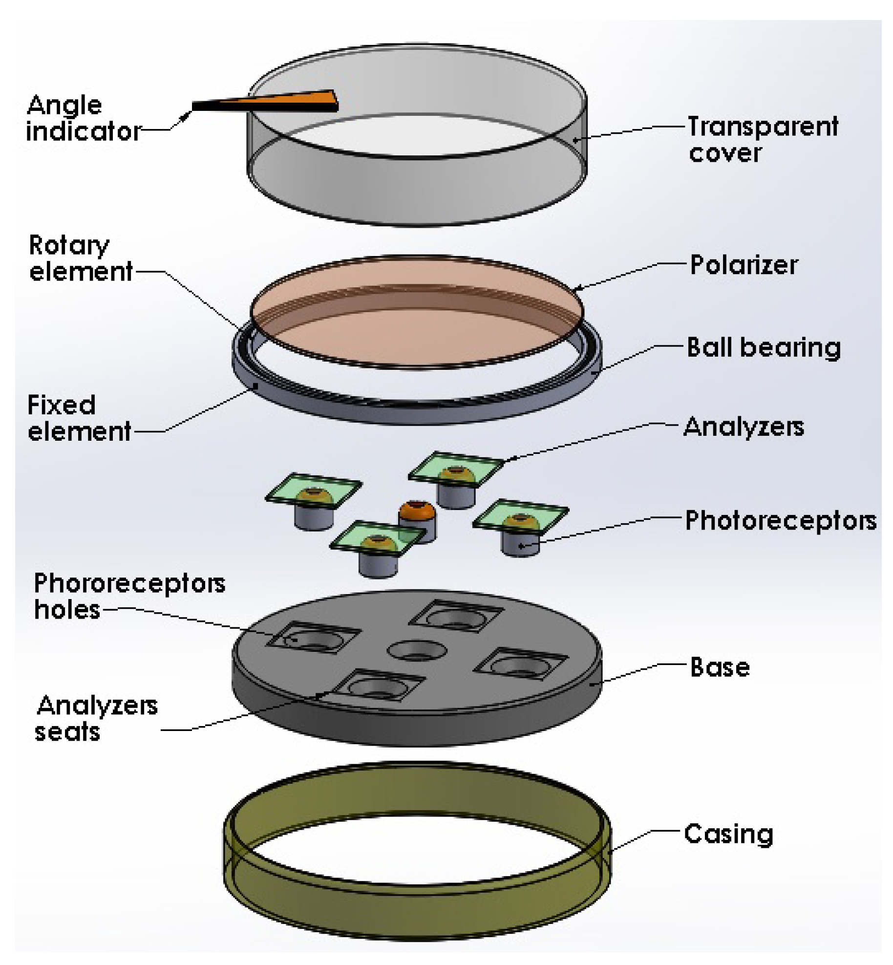
In
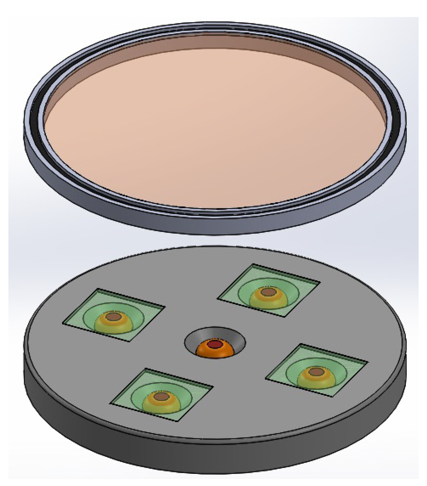
Figure 1, we have an exploded view of the device where each of its constituent components can be appreciated. In this figure, we have a base that has five holes to accommodate the five photoreceptors whose information constitutes the five inputs of the proposed neural network. The base also has four seats to house the analysers, which means that the central photoreceptor is without an analyser. On top of the base, a bearing is also seated, which allows the rotation of a polariser, since the latter is attached to the rotating element of the bearing. A housing unit solidly connects the base to the fixed element of the bearing. Finally, a transparent cover attached to the rotating element allows the entry of light from the outside. As an additional element, the cover can contain an arrow indicating the reading of the angular position, which must coincide with the output of the neural network.
In
Figure 2, the main elements of the basic idea of the sensor are shown. Both the photoreceptors and the analysers within their bases, and the rotating polariser in its position are displayed.
In
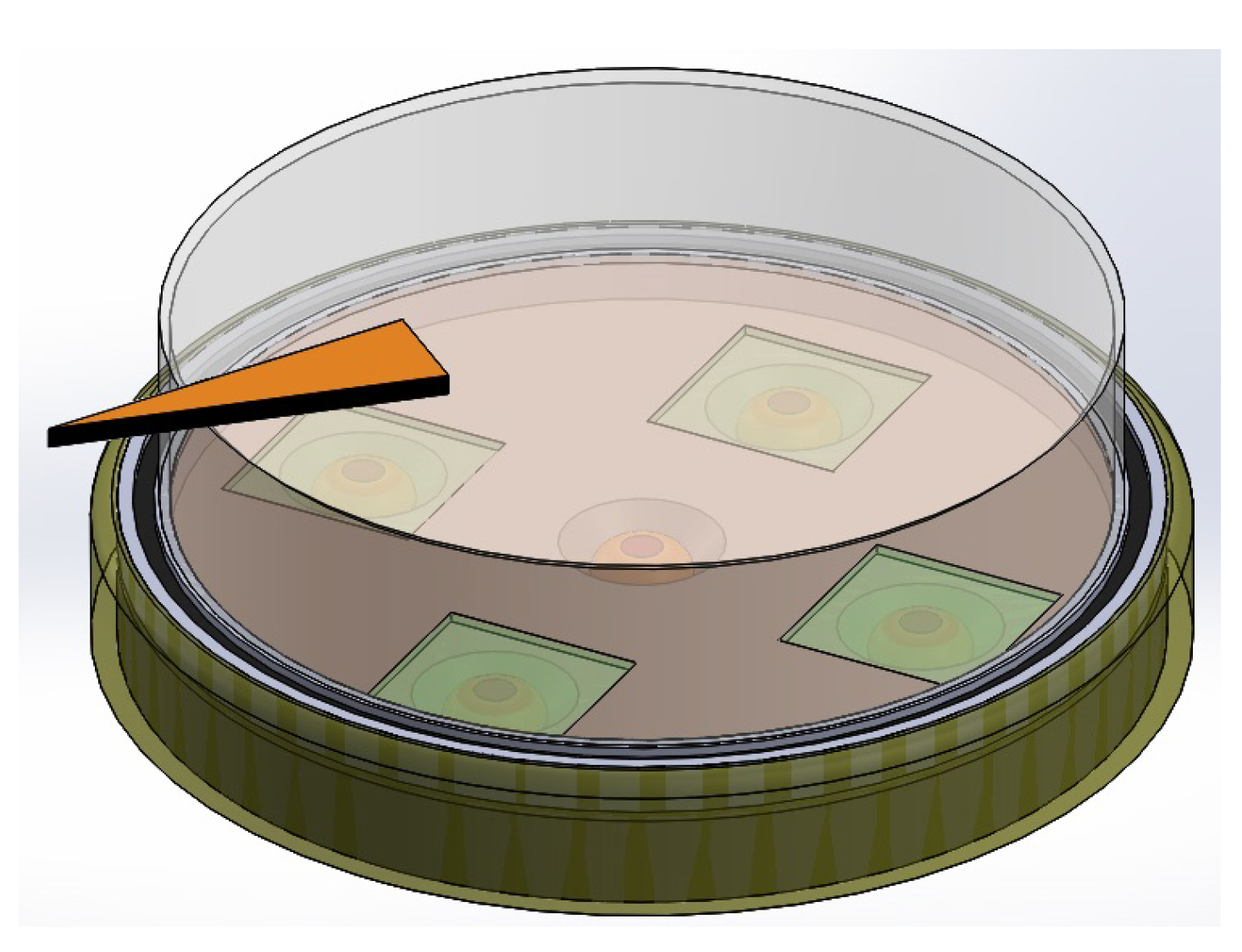
Figure 3, we have the assembly of all the constituent elements of the sensor.
To explain the operation of the encoder, we will begin by saying that when a beam of light passes through two consecutive polarisers (the first of them called "polariser" and the second one called "analyser"), the resulting light intensity
is quantified by the Malus’ law
where
represents intensity of light of reference,
i.e., the intensity of light before any polarization, and
is the angular position of the polariser (see [
17,
18]). Nevertheless, such arrange allows to measure an angle in the interval
, and to solve this major drawback, the studied sensory device consists of four phases which follow the Malus’ law, with phase shift of
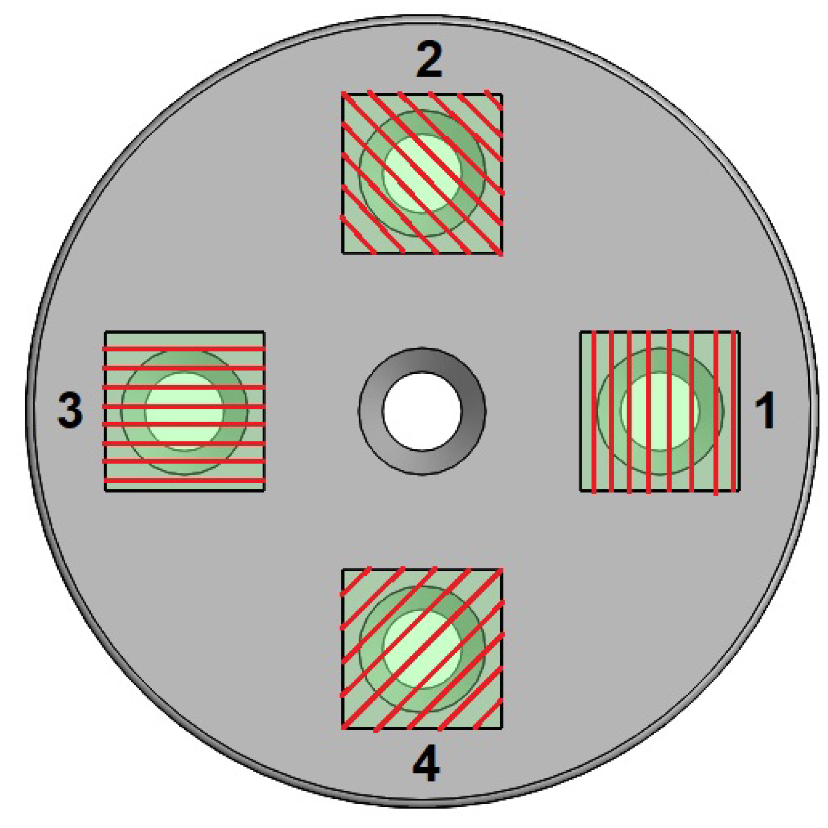
as depicted in
Figure 4. It should be clarified that the red grids are only a representation for didactic purposes of the polarization axes since they are not perceived by the naked eye.
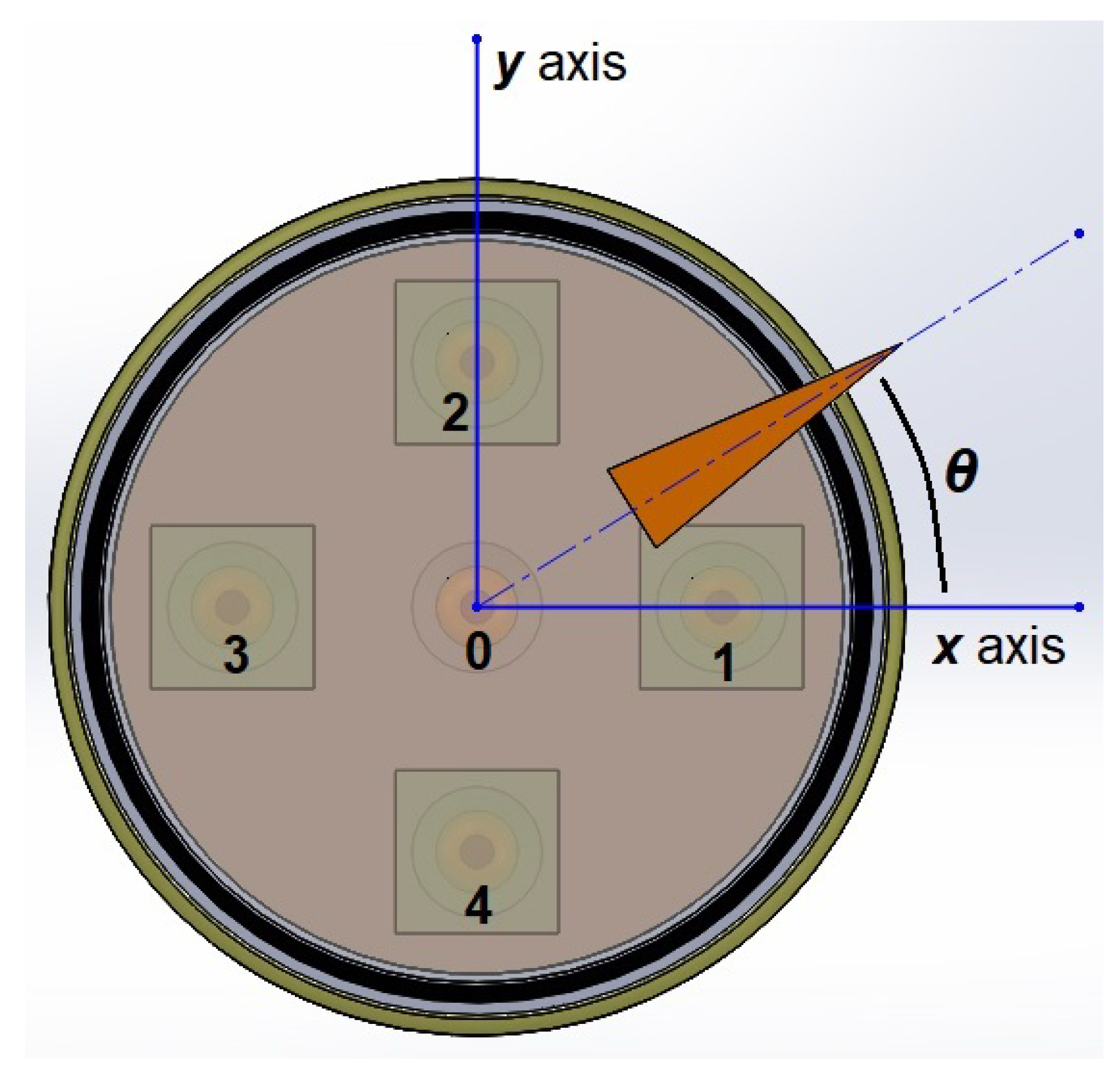
In this way, the light intensities coming from the reading of each photoreceptor will allow the identification of the angle generated by the polariser, as depicted in
Figure 5, whose value is in the interval
.
According to the equations relative to the phase shift polarization, in theory, the angle
can be obtained by
where the intensity of light for each of the four phases is modelled by
However, the use of the algorithm shown by the above equations only works under laboratory environment since the following conditions in the encoder’s manufacturing must be strictly met:
1. The phase shift angles must be exactly 45 degrees for 4 phases, 120 degrees for 3 phases, etc.
2. Both polarisers and analysers must be free of optical aberrations and must be manufactured perfectly.
3. The photoreceptors must present linear readings according to the intensities marked by Malus’ law and must be free from phenomena of saturation and hysteresis.
4. The device must work free from disturbances and noise.
Obviously, for heavy-duty work conditions in the industry, these conditions are practically impossible to meet. Therefore, a method based on artificial intelligence is proposed to obtain the reading of the encoder’s angular aperture.
Summarizing, according to the polyphasic encoder depicted by
Figure 1,
Figure 2,
Figure 3,
Figure 4 and
Figure 5, the problem to solve is focused on designing and implementing adequate ANN’s endowed with a machine learning technique, with an input vector of five intensities of light and one output to predict the angular position, such that none of the four conditions enumerated above, require necessary to be fulfilled to get an excellent encoder’s performance.
3. Neural Networks design
This study presents several neural networks instead of a single one, with the purpose of observing the behaviour of each of them and obtaining conclusions about the dimensions and characteristics that a neural system oriented to perform the proposed task should have.
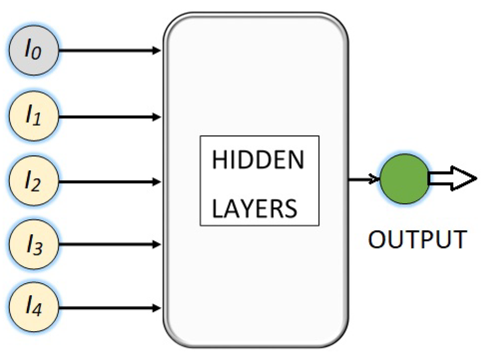
Thus, a set of four neural networks are being developed to perform a regression task, where the input of each is a vector with the values of five light intensities and the output is a predicted angle, as it is shown in
Figure 6, where the hidden neural layers are the ones that will process the input information and transform the data in a way that can be used to generate a good angle prediction. The number of hidden layers and the number of neurons in each of them is an hyperparameter that must be determined through experimentation and fine-tuning.
Figure 4 and
Figure 5, show the four phases from which the intensities of light
originate, along with the light’s intensity of reference
.
The first NN is a network with its five respective inputs, a single hidden layer with two neurons, and finally an output node. This is represented in
Figure 7.
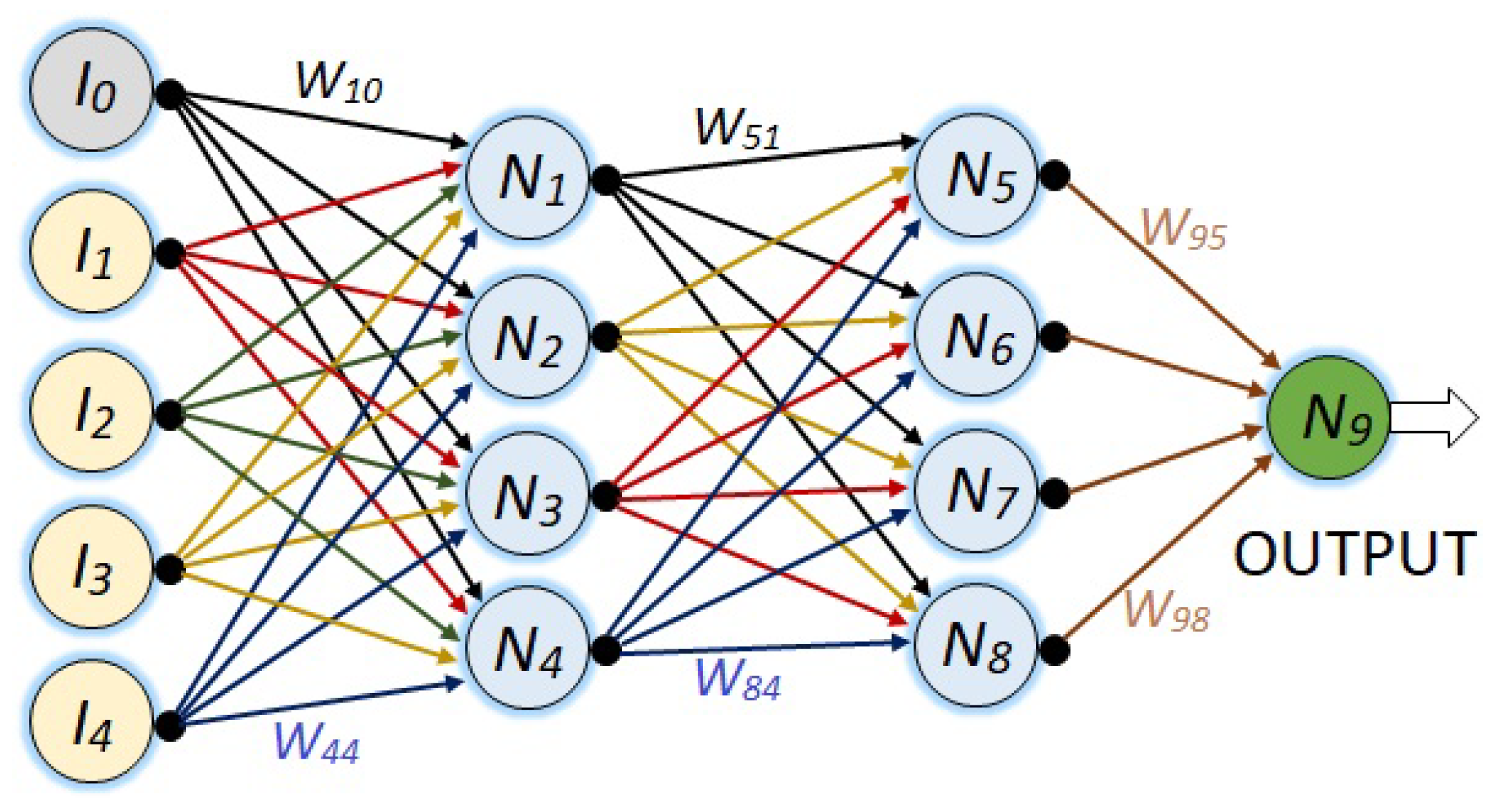
Figure 8, shows a more complex neural network with its five respective input nodes, two hidden layers of four neurons each, and its respective output node.
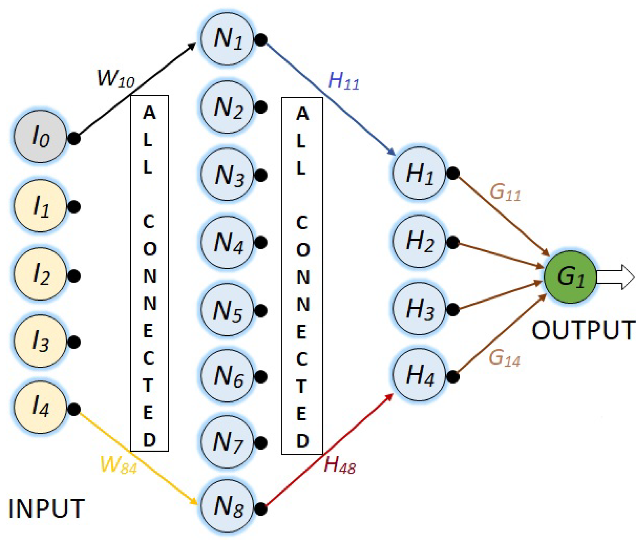
Figure 9, shows the most complex network of the last three, since it is similar to the previous network, but its first hidden layer has eight neurons instead of four.
In this last
Figure 9, not all connections are shown in order to preserve the quality of the figure. However, in all the networks shown, it is assumed that all the nodes in one layer are connected to all the nodes in the next layer and to all the nodes in the previous layer.
Finally, in
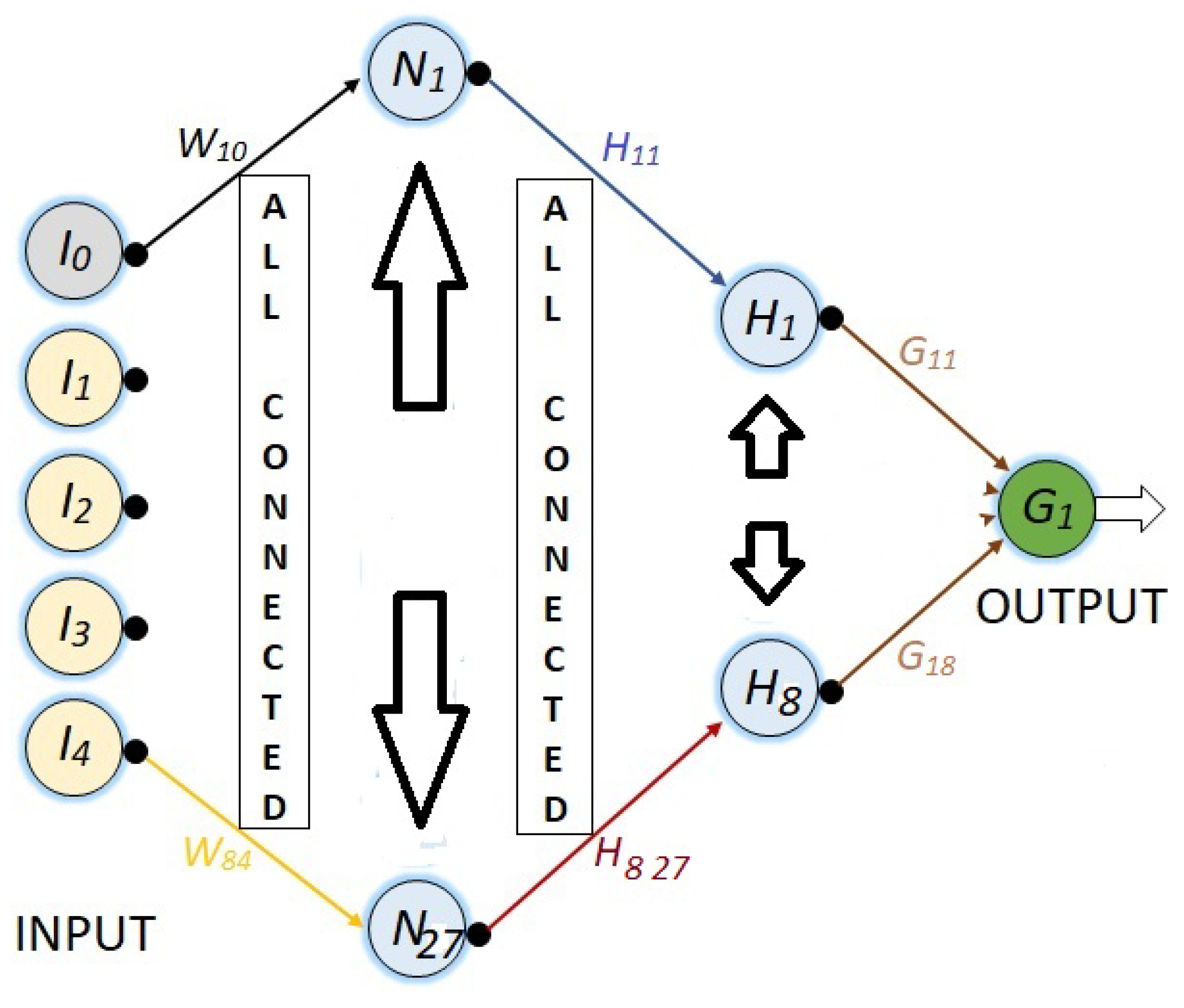
Figure 10, a NN with 36 neurons is presented, where the firs hidden layer has 27 and the second hidden layer has 8 neurons. As in the last NN, all nodes from one layer to the next are connected, such that there are 359 synaptic weights.
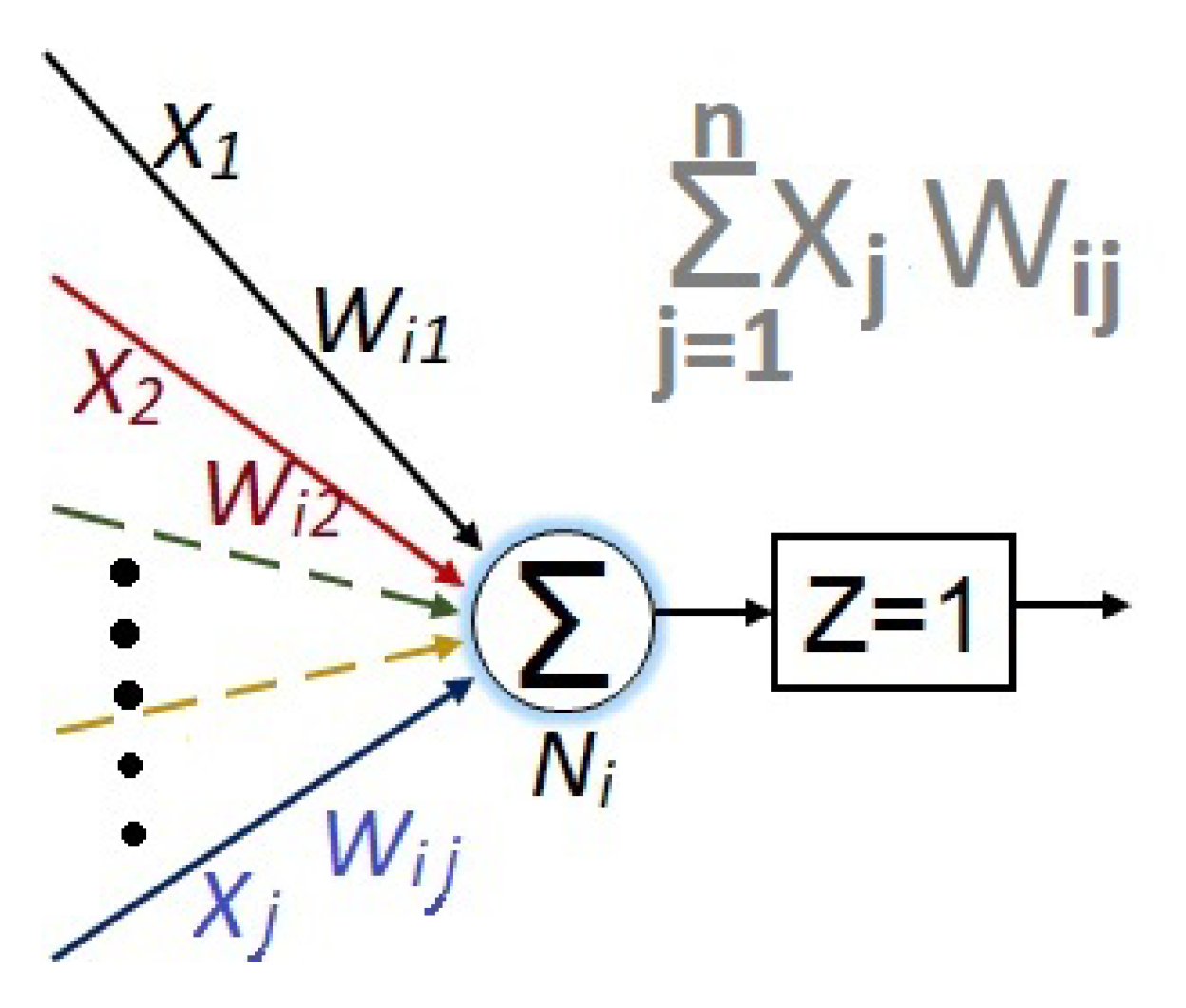
For all the NN’s, the synaptic weights are represented with , where i represents the destination node and j the source node.
Meanwhile, the activation functions for all the neurons in the network are the constant 1, since after attempting to work with other activation functions, the network does not work correctly. The activation functions that were tested were tanh, functions, and combinations of exponentials with sin and cos functions. Thus, a first conclusion is that the neural network for this type of application does not require the introduction of these types of nonlinearities.
Even more, the numerical value for each node is given by:
which is graphically exemplified in
Figure 11.
3.1. Training algorithm
To train the network, a labelled dataset containing values of light intensity and corresponding angles being predicted will be needed. These data will be used to adjust the weights of the network and improve its ability to make accurate predictions. The goal will be to minimize the error between predicted angles and actual values.
To make this job, the total error must be obtained with
where
is the real value of the angle, and
is the predicted angle. After this, the total error
must be retro propagate to the NN multiplying the error corresponding to each node by its respective synaptic weight
.
When the error has been retro propagated, the synaptic weights must be updated by
where
is the learning rate.
The updated numerical values for each node
is obtained by
When the output value has been obtained, this process is repeated using many training examples.
Once the neural network has been trained, it can be used to make predictions on new sets of data. The accuracy of the network will depend on the quality of the training data and the architecture of the network.
3.2. Training example
The last algorithm (
8)–(
10) is now exemplified to train the NN given by
Figure 8. However, to train the NN’s of
Figure 7 and
Figure 9, the procedure is the same. 1. The first step is the obtaining of the total output using (
8) in three consecutive stages.
a) To get the value for each neuron at the first hidden layer (
):
b) To get the value for each neuron at the second hidden layer (
):
c) And finally, to get the value for the total output of the NN:
The total output (
) is the predicted angle, and it is compared with respect to the expected actual value
, which is the total error
2. The second step consists in the retro propagation of the total error to each connection of the NN, also in three reversed stages.
a) To retro propagate the error from
to the second hidden layer (
):
b) To retro propagate the error from the second hidden layer to the first hidden layer (
and
):
c) And finally, to retro propagate the error from the first hidden layer (
and
), is also used (
16).
3. The third step consists in the updating of the synaptic weights using (
9) and (
15)–(
16) in the following forwarding direction.
a) From the input vector to the first hidden layer (
and
):
b) From the first to the second hidden layer (
and
):
c) And finally, from the second hidden layer to the output (
):
4. The last step is the obtaining of the new output and in some sense it is simultaneous with step 3, because the updating of the synaptic weights require also the update of the the last outputs, with the exception of the total output which must be obtained using (
10).
3.3. Machine learning strategy
The acquisition of information vectors for training a neural network is a time-consuming and laborious process. For this reason, it is desirable for the machine to have the ability to learn by itself using some strategy. A mathematical based strategy to use the given equations (
3)–(
6) to automatically obtain the values of light intensities for each angular value is desired.
To carry out this process, it is necessary to implement a system where the angle value is updated, and with that value, the light intensities are obtained. Subsequently, the network is trained with those values, and this entire process is repeated automatically in a repetitive manner.
In the initial step, an arbitrary value is assigned to the angle , and the given equations are used to calculate the light intensities , , , . Then, the angle is incremented/decremented to get , leading to the modification of the light intensities to , , , , and the synaptic weights are adjusted accordingly.
This process of updating the angle, calculating the new intensities, and modifying synaptic weights is repeated for
n iterations:
However, as has been said, algorithms based on mathematics must meet a series of requirements to be exact and precise. Therefore, the same principle can be implemented by means of a mechanical operating device, from which the light intensity values are associated to each determined angle, and automatically obtained.
3.4. Implementation example
This implementation example is done in Matlab’s Simulink program and involves applying the equations (
11)–(
19) that describe the neural network in the
Figure 8 along with its training, and the machine learning strategy (
20) is also a fundamental part of this example.
The same principles and programming techniques from this example are followed to program the other neural networks proposed in this work.
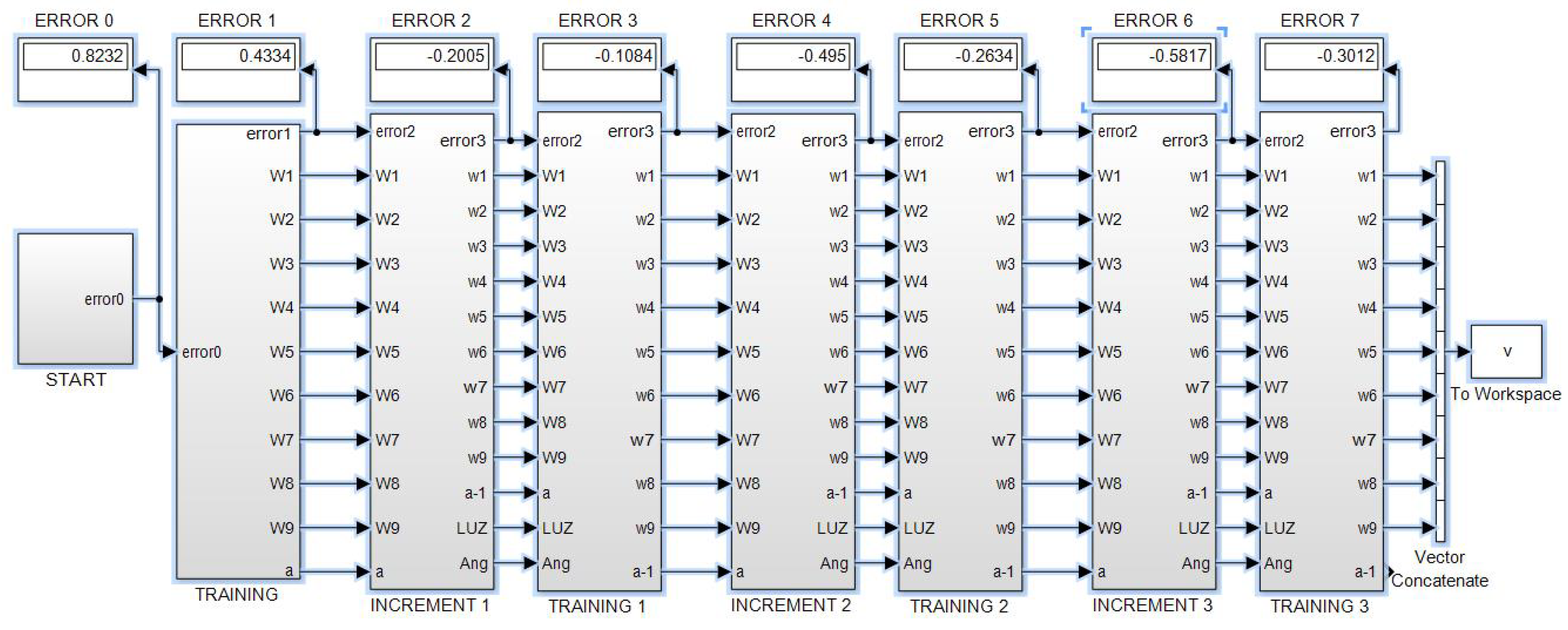
Figure 12, shows the root program, which consists of eight subsystems. The first subsystem contains the neural network with five inputs, two hidden layers with four neurons each, and one output neuron.
The second subsystem contains the program for the first training cycle, where the error is backpropagated, synaptic weights are adjusted, and an output is obtained with reduced error.
The third subsystem contains a program that calculates the corresponding light intensities for an angle that has a different value than the initial one. Meanwhile, the fourth subsystem contains the training program for this third subsystem, following the same description as for subsystem two.
The fifth and sixth subsystems are a repetition of the third and fourth subsystems. Similarly, the seventh and eighth subsystems are also a repetition of the previous ones, allowing for the addition of the desired number of pairs.
The , represent vectors of synaptic weights for each of the nine neurons in the exemplified network, totaling forty parameters that are updated in each angle update and its corresponding training. This process continues until the end of the sequence, where the values of the synaptic weights are stored in Matlab using the "To Workspace" instruction to initiate new training cycles that progressively reduce the error.
If, for example, we start with an angular value of 17 degrees and program a negative increment of one degree, then subsystem eight will provide us with adapted synaptic weights and corresponding light intensities for 14 degrees. However, prior to this, the network has been trained for values of 15, 16, and 17 degrees. If we repeat this process a sufficient number of times, it is expected that the network will be trained to predict angular measurements close to the 14-17 degree interval when given a vector of light intensities as input.
Both the accuracy and precision, as well as the range of the angle to be predicted, depend on the capacity of the neural network. In other words, a neural network with small hyperparameters and insufficient architecture will be able to predict within small angular intervals with wide margins of error. Meanwhile, powerful neural networks can predict with high accuracy and precision within the full 360-degree range detectable by the sensor.
Moving on to the next
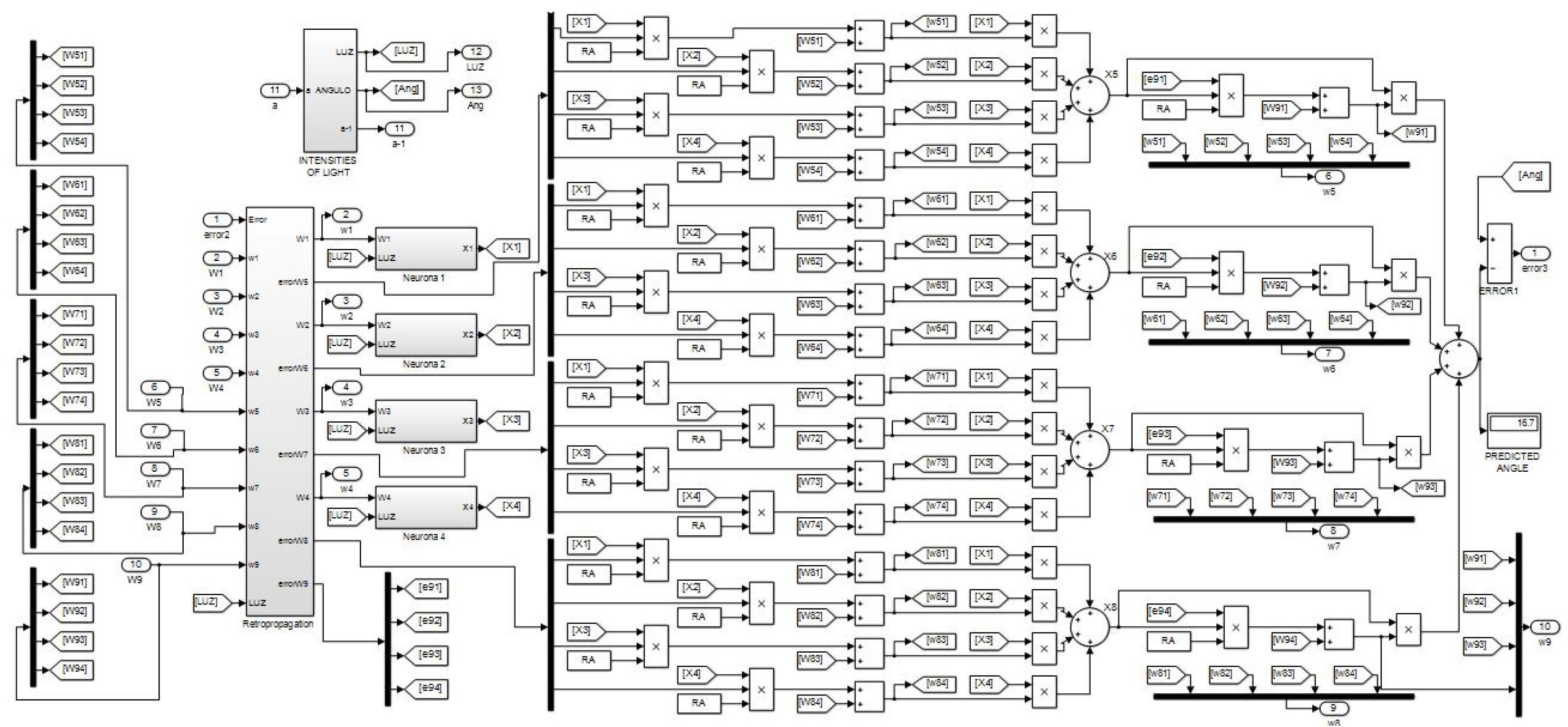
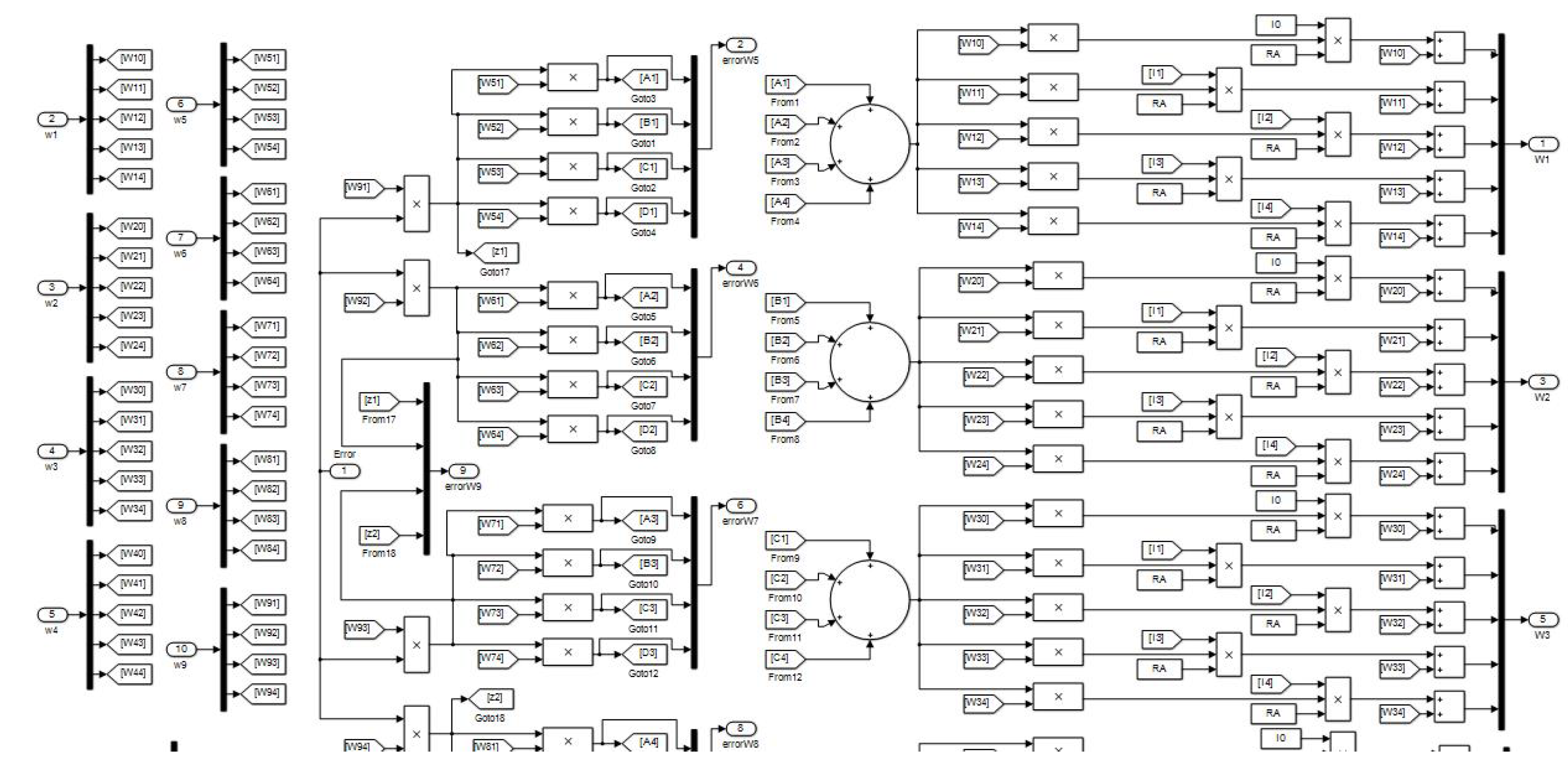
Figure 13, we have the block programming of what is contained in subsystems three, fifth and seventh of the previous
Figure 12. In program of
Figure 13, we can see other subsystems, one of them containing the error backpropagated inherited from the previous subsystem, another one containing the calculation of light intensities for new angles, and four others containing the neurons of the first hidden layer. The four summation nodes appearing on the right-hand side represent the four neurons of the second hidden layer. The rightmost summation node represents the output neuron, where the calculation of the total error at that stage is performed. As it can be seen, the synaptic weights are updated before the calculation of each neuron’s output.
In the next
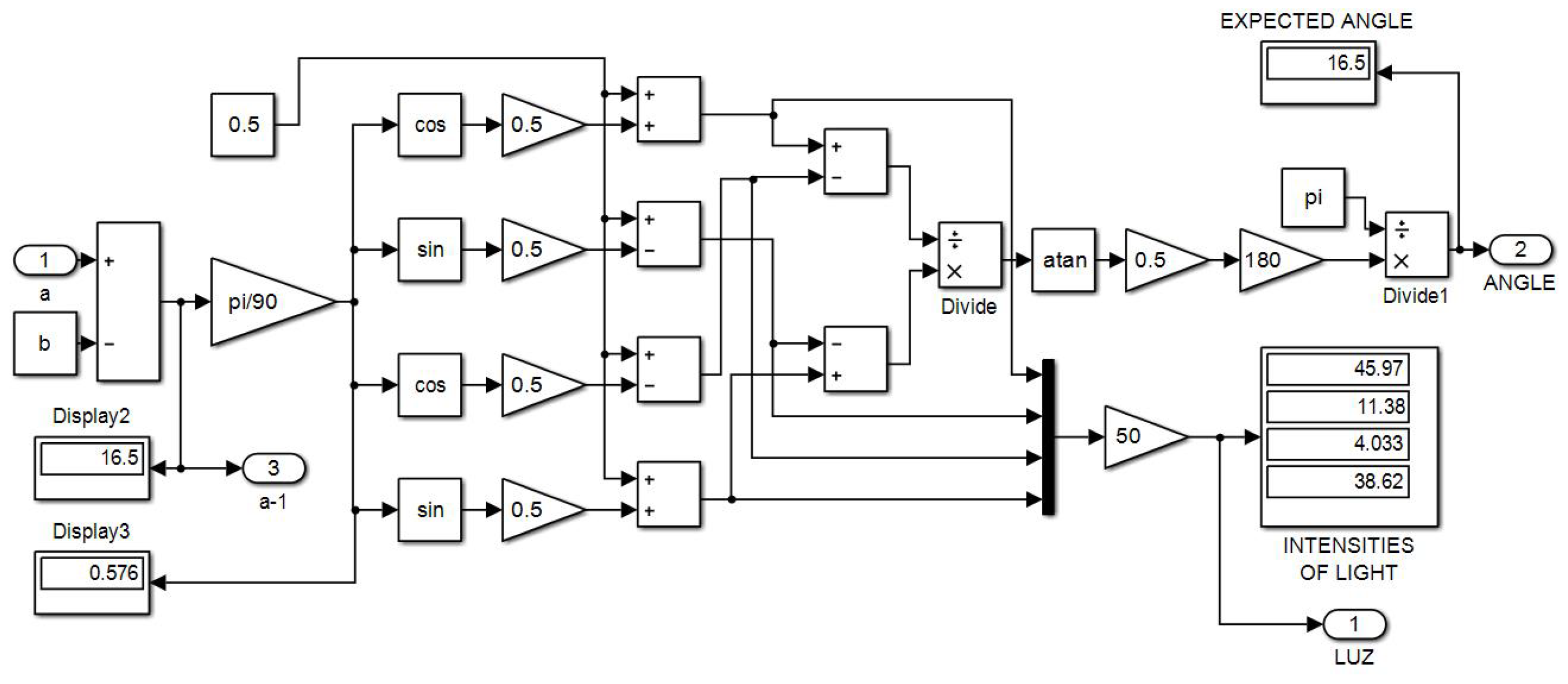
Figure 14, the program within the subsystem "Intensities of light" is shown, which corresponds to the calculation of the light intensities that should correspond to each angular measurement, according to what was explained in the subsection "Machine learning strategies".
The input "a" is the angle stored in the program’s working memory, starting with an arbitrary initial value. Meanwhile, the constant input "b" is the increment/decrement that will be applied to the angle in each iteration of the training process. By adding/subtracting "b" from "a," an updated value of "a" is obtained, which will change throughout the machine learning cycle.
If we take away the subsystem of
Figure 14 from
Figure 13, then, subsystems fourth, sixth and eight of
Figure 12 are obtained,because the exclusive training blocks do not include update of angle and light intensities. The same can be said for block two in
Figure 12, however, the first training block does not inherit previous synaptic weights.
The block program within the "Retropropagation" subsystem is shown in
Figure 15, where the items 3 and 4 of the "Training example" can be seen in a diagram block.
Finally, the
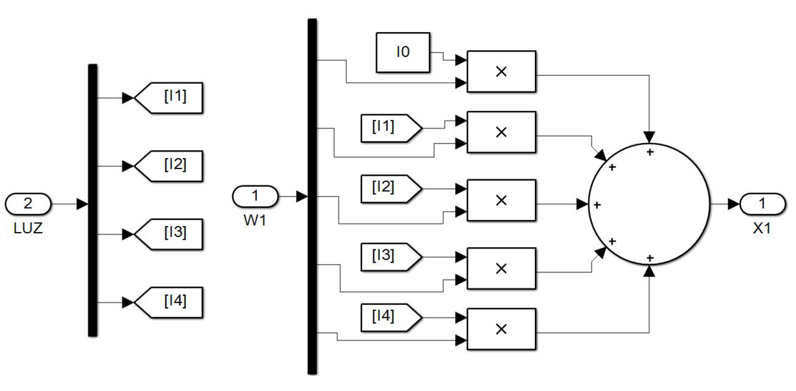
Figure 16 shows the interior of a neural subsystem where it can be observed that the only constant value is
. In this case, we are dealing with a neuron in the first hidden layer. As you can see, the synaptic weights converging on the node are multiplied by the light intensities from the encoder. The neurons in the second hidden layer have a similar structure but with four inputs coming from the first hidden layer.
Up to this point, the neural network of
Figure 8 has been exemplified using block diagrams and explanatory text, allowing the reader to implement this neural network on their own. Finally, as you may have noticed, for this program to work, two additional Matlab programs in .m format are required. The first program should be executed before running the block program and should contain the parameters "a" and "b" along with their initial light intensity values, the learning rate "RA," and the initial synaptic hyperparameter. The second .m program should be executed after each run and should contain the updated values of the synaptic weights sent to Matlab using the "To Workspace" instruction.
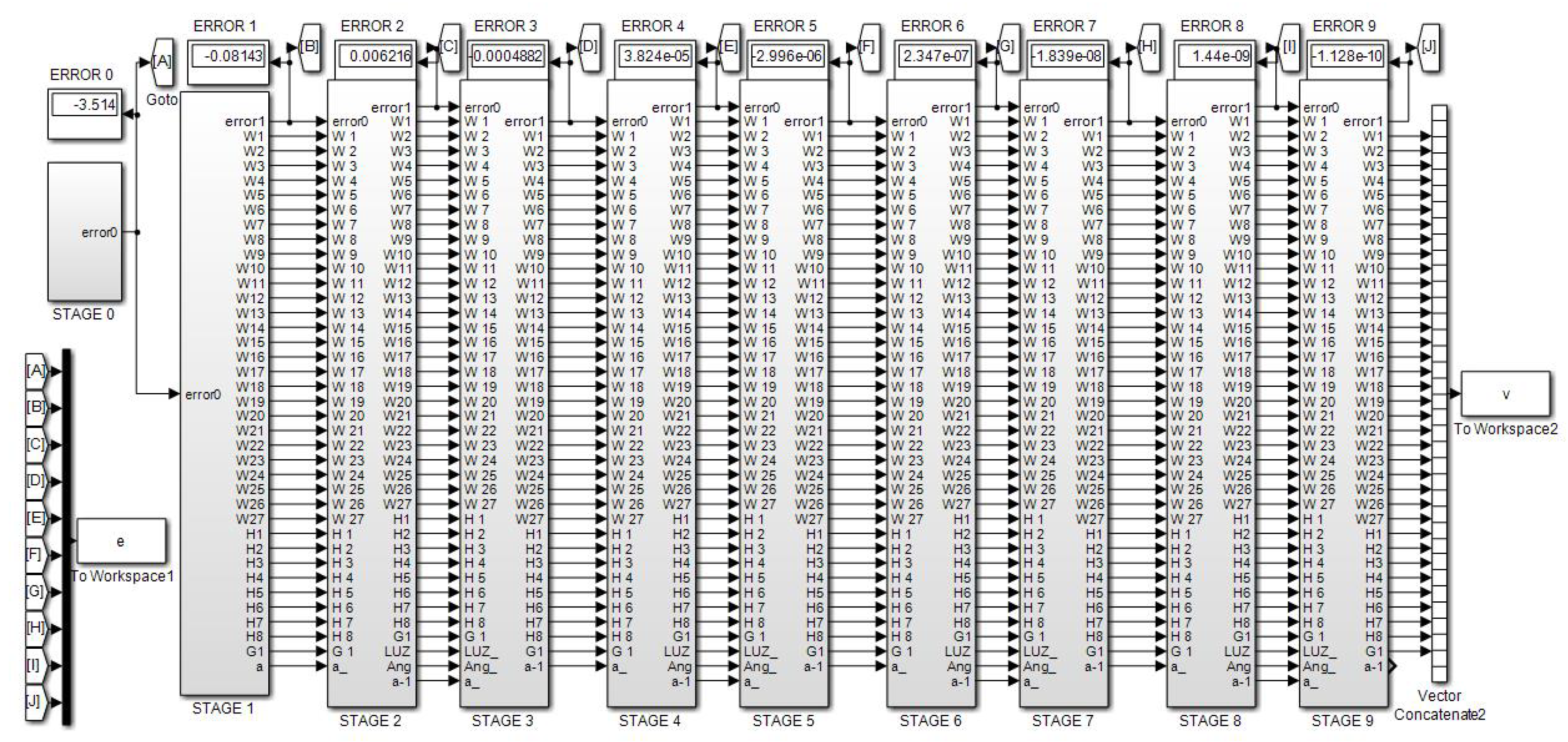
Now let us show another example with an arrange made for the NN of
Figure 10 endowed with 36 neurons, which corresponds to the program shown by
Figure 17, which has a different purpose than the one in the
Figure 12. Every "Stage" block of
Figure 17 has the same structure of the "Increment" block in
Figure 12, and both kind of structures will be used to obtain simulation results.
Observe that the hyper parameter for this NN is conformed by 359 synaptic weights.
Once the NN’s have been trained, the hyper parameters can be stored in a database to be used when they are required. In the Appendix, the initial synaptic weights along with the trained ones are provided for every NN.
Note.- The synaptic weights for do not appear for the first NN (3 neurons) since heuristically it was detected that they did not provide benefits for their good performance.
4. Performance results
The implementation for simulation purposes has been performed for the four networks shown in the
Figure 7,
Figure 8,
Figure 9 and
Figure 10, and below performance results are presented for an interval from 13 to 17 degrees, and symmetrically from 17 to 21 degrees, using the corresponding light intensity vector as system input. For this purpose, each NN has implemented in two versions, the first one with the structure shown by
Figure 12, and the second one with a structure as shown in
Figure 17.
The intensities of light for every angle
were obtained using equations (
3)–(
6), and taking
as the parameter for all simulation results.
Because neural networks behave quite strangely depending on their architecture and size, it is difficult to establish benchmarks between them. However, based on its functionality within this application, we will try to establish a way to perform comparisons.
Using the novel machine learning technique expressed by (
20) and illustrated by
Figure 12, a performance comparison between NN2, NN3 and NN4 is given in
Table 1 (NN1 is not considered because it presents low performance when it is trained for intervals).
The intervals in the first column of the referred table have a lower value, a central value and an upper one, such that the central value for every interval has arbitrary selected as 17 degrees for this study. This central value increases or decreases symmetrically in one, two, three and four degrees to obtain four intervals.
Remember that every Increment block increases/decreases "b" degrees (for this case b=1) from the previous block (accordingly with
Figure 14), such that the performance of the first interval is obtained taking data from the Training 1 block, the second interval takes data from the Training 2 block, wile the third interval takes data from the Training 3 block, shown in the mentioned
Figure 12.
The table indicates the minimum values obtained for the training at the extremes of every interval, taking into account the better learning rate (LR) heuristically found and used for each case.
Certain remarks can be drawn from
Table 1:
1. When the range of the interval is widened, the minimum error increases. Nevertheless, an increase in network capacity helps in reducing error.
2. The neural network of 36 neurons performs a little better than the others, however, the computational cost increases considerably. 3. Strangely, the network of 9 neurons is more efficient than that of 13, which supports the fact that the architecture of the network influences its efficiency.
4. Both the errors and the training rates of the network of 13 neurons are higher than those of the others (for the last three intervals), which supports the idea that both concepts are directly proportional to each other for a neural network (also see that in the first interval it is reversed).
5. An additional remark obtained from the research process, is that every one of the presented Neural Networks are extremely sensitive to small hyper parameter changes, since a single change of some initial synaptic weight value can lead to different NN behaviour. Nevertheless, those of
Table 1 are the better results obtained after many hours of tune and adjustment. Thus, it is concluded that a lot of time is required to tune the NN’s and to find their optimal functioning.
Once a comparative analysis between the different neural networks has been carried out, now let’s review the error that each of them throws when they are trained around a specific region. The angle must be specified by the user assigning the desired angular value "a" and "b=0" in the Matlab console directly or running beforehand a .m file containing this information, which feeds the subprogram shown in
Figure 14, and after running the program depicted in
Figure 17.
For this case is selected "a=17" (which with
can be used to detect angles in the range
–
). The corresponding intensities of light are automatically obtained by subprogram of
Figure 14, and the training process starts with the machine learning technique.
In the
Table 2,
Table 3,
Table 4 and
Table 5, the first column corresponds to the Learning Rate (LR), and the first row to the training stage from the initial reading (0) to the 9-th learning stage.
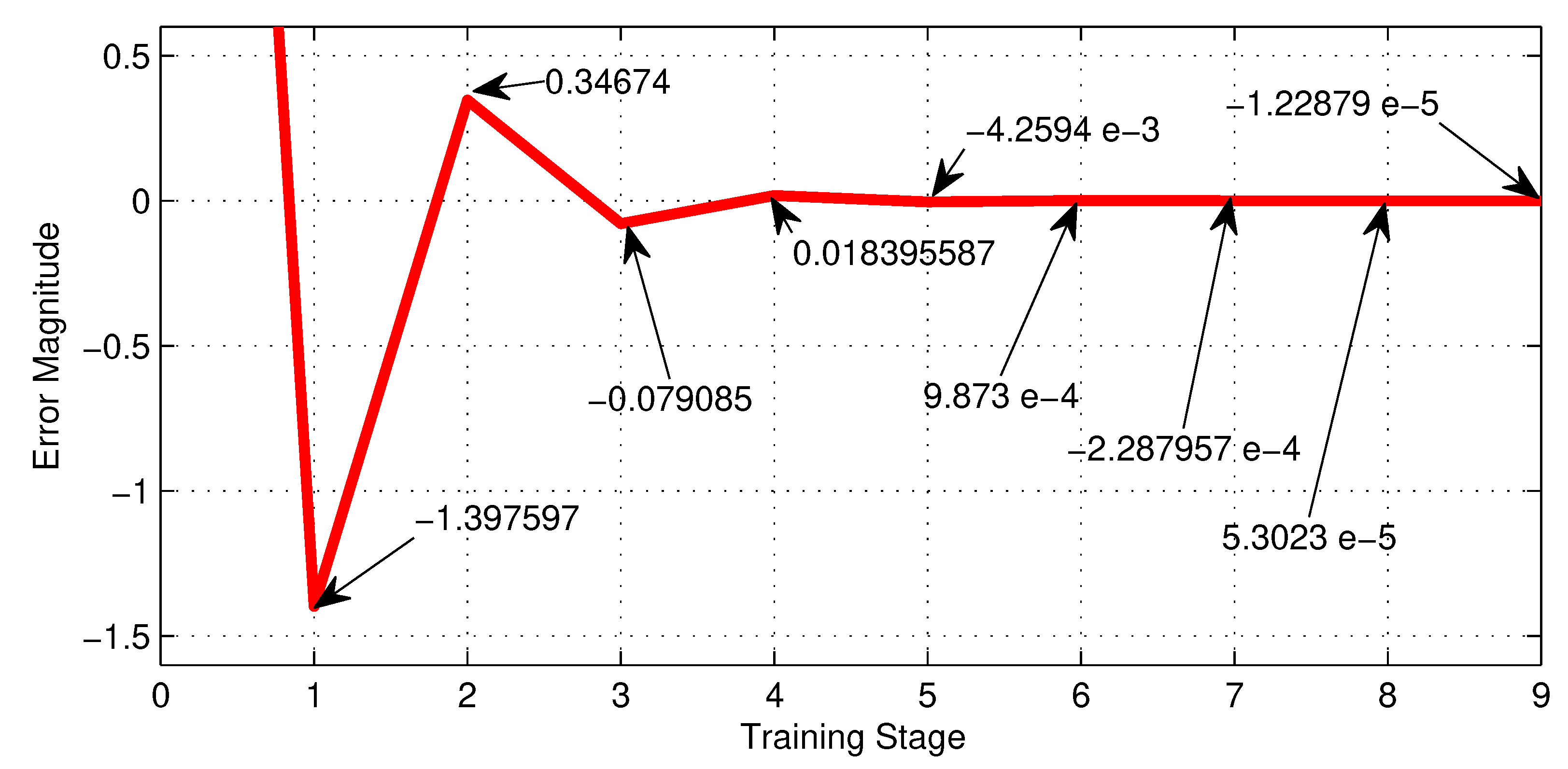
Table 2, shows the training performance of the first NN shown in
Figure 7, where the best LR is
and reaches a minimum error of
.
Figure 18, shows graphically the 4-th row of
Table 2.
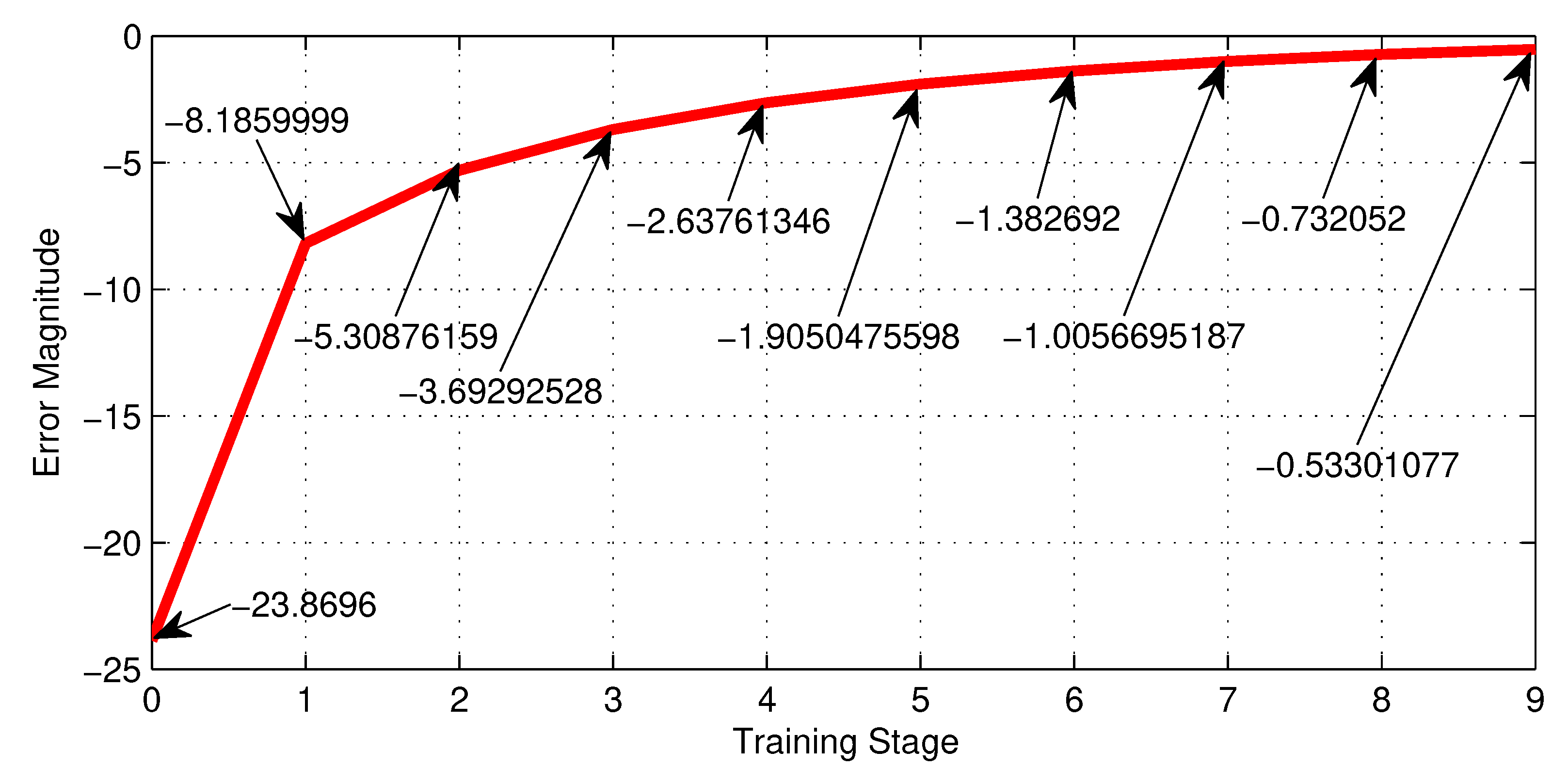
Table 3, shows the training performance of the first NN shown in
Figure 8, where the best LR is
and reaches a minimum error of
.
Figure 19, shows graphically the 5-th row of
Table 3.
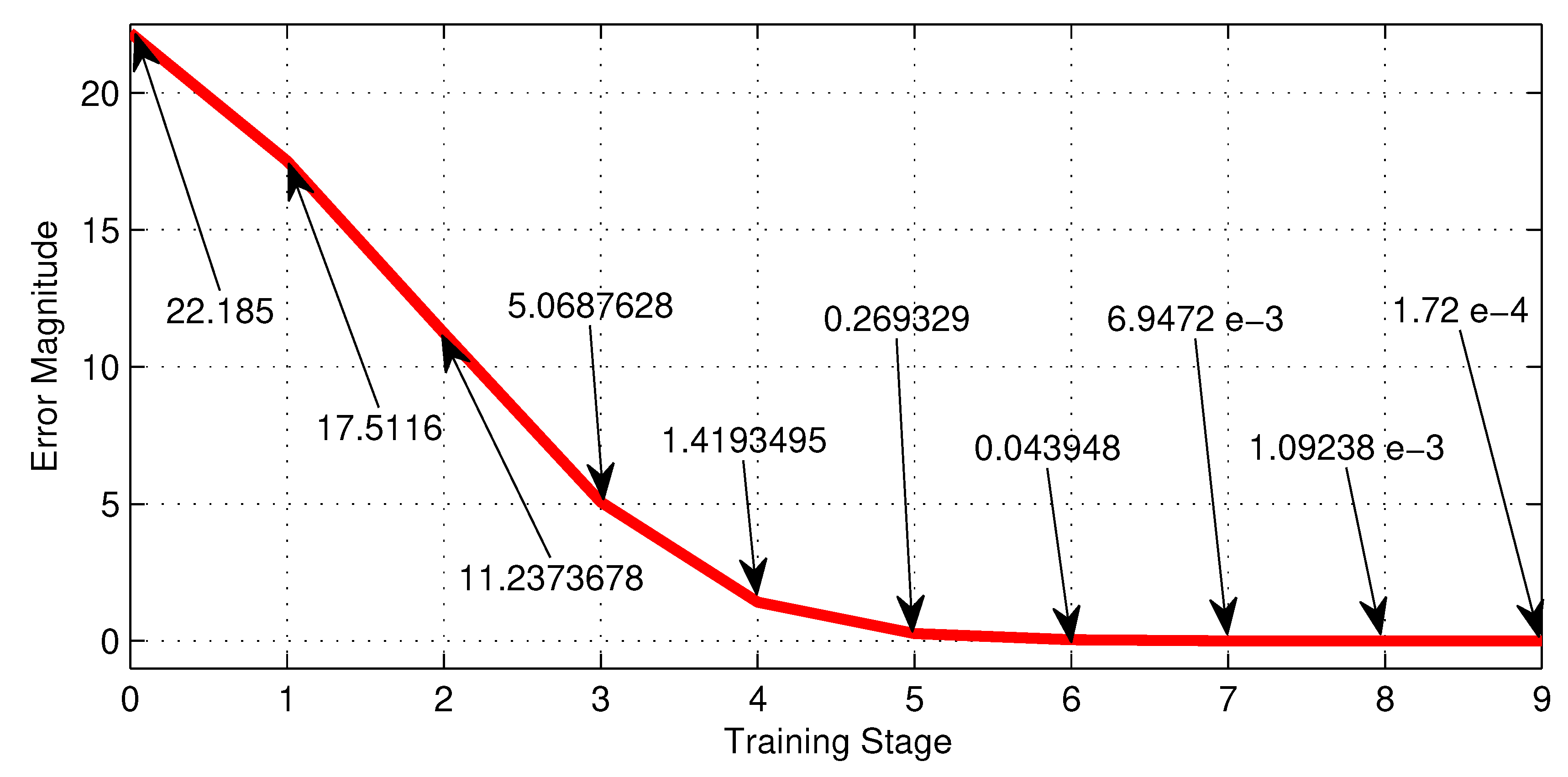
Table 4, shows the training performance of the third NN shown in
Figure 9, where the best LR is
and reaches an error of
.
Figure 20, shows graphically the 5-th row of
Table 4.
Table 5, shows the training performance of the third NN shown in
Figure 10, where the best LR is
and reaches an error of
.
Figure 20, shows graphically the 3-th row of
Table 5.
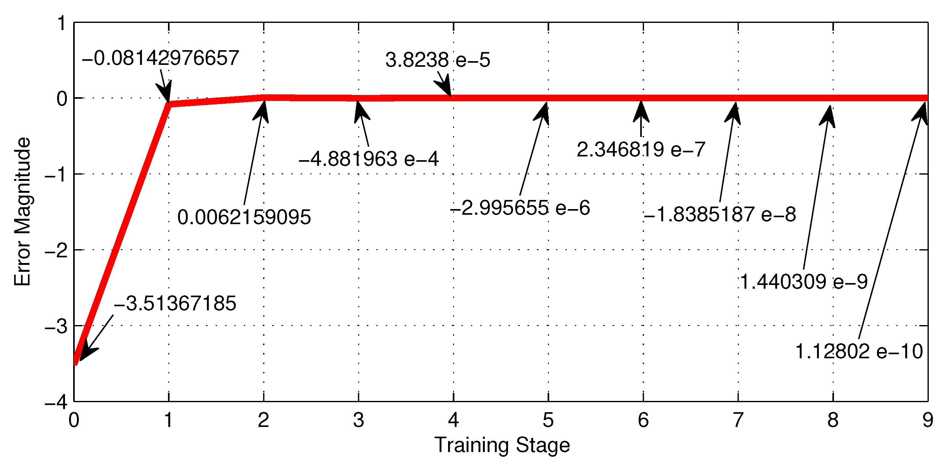
Figure 21.
Error behaviour of the NN with thirty six neurons given by
Figure 10 along the training stages from the initial 0 to the 9-th.
Figure 21.
Error behaviour of the NN with thirty six neurons given by
Figure 10 along the training stages from the initial 0 to the 9-th.
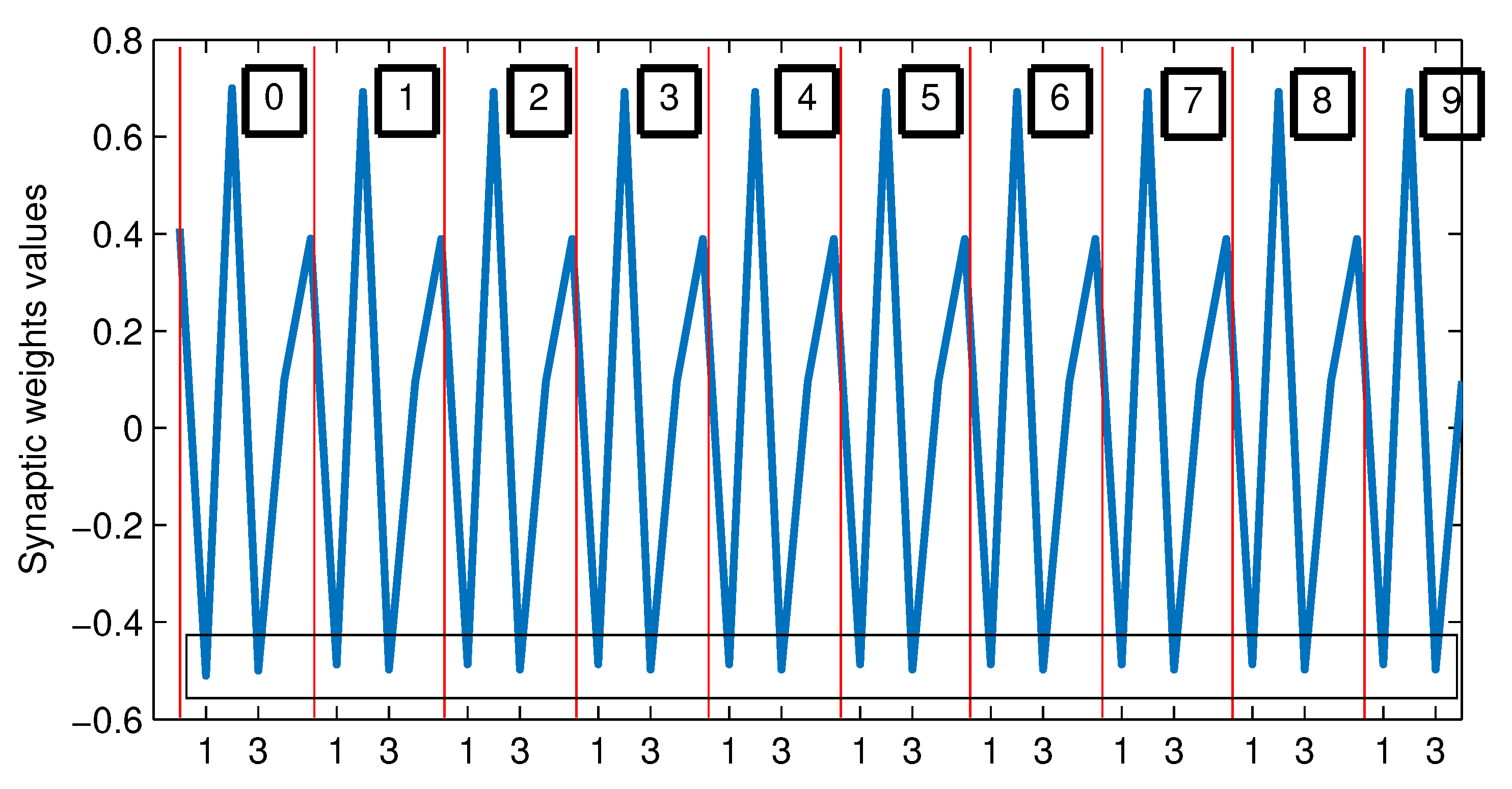
Important remarks can be obtained from the last study...
Figure 22.
Behaviour of the synaptic weights values of from the 0-th to the 9-th training stage.
Figure 22.
Behaviour of the synaptic weights values of from the 0-th to the 9-th training stage.
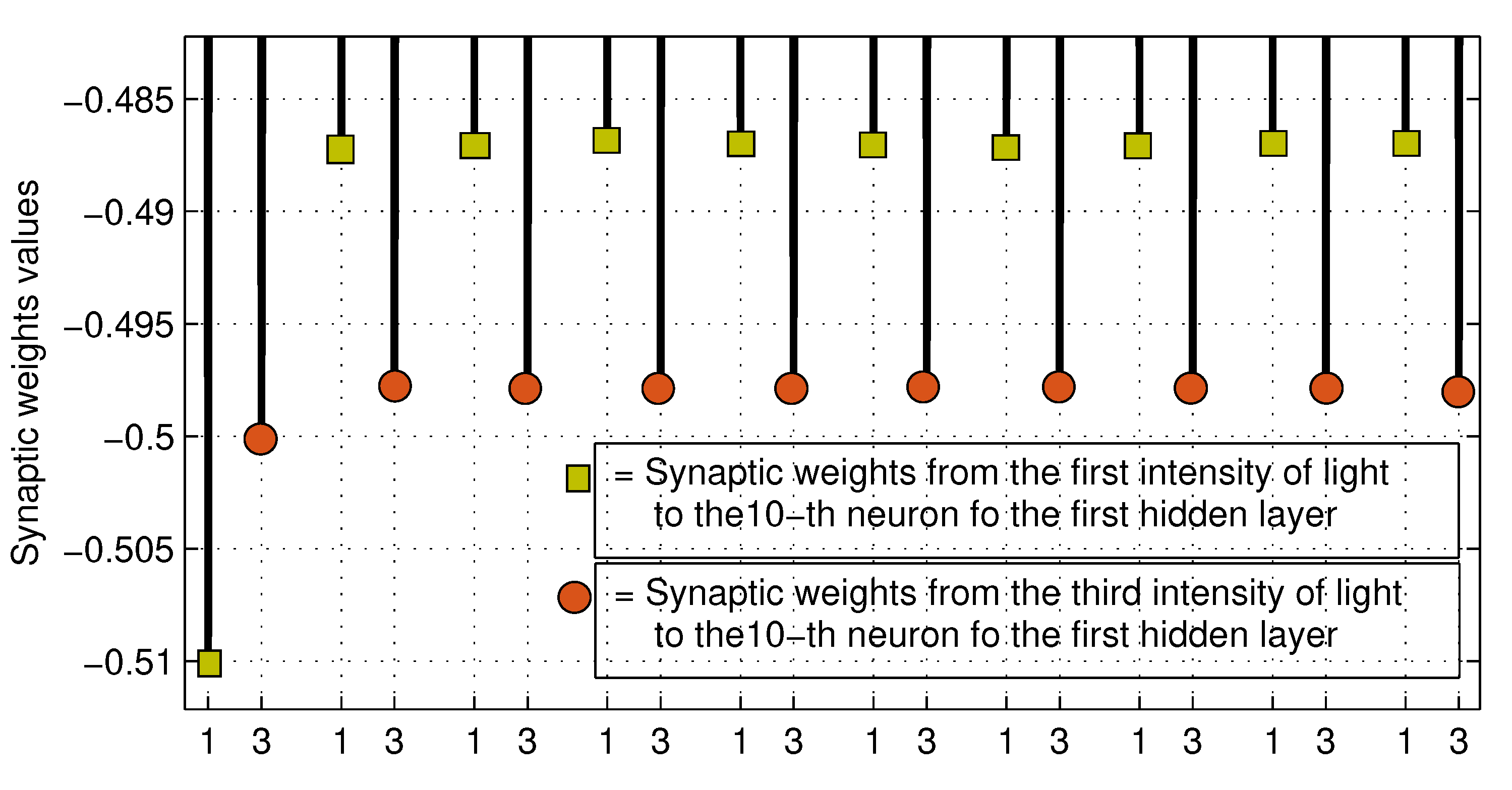
Figure 23.
Enlarged view into the rectangle at the button of
Figure 22.
Figure 23.
Enlarged view into the rectangle at the button of
Figure 22.
5. Intervals management
In
Table 6, the full range from 0 to 180
o is partitioned in 16 intervals of
each. In the first column the angular position is marked, and columns 2, 3, 4 and 5, the corresponding intensities of light are given (taking
). Observe that every interval has a defined and unrepeated relationship between the four intensities of light. For example, the first interval goes from 0 to
and the relationship between the corresponding intensities of light is:
Obviously the beginning of the first interval, or in other words, the zero degrees can be located at any position on the circumference, so it is possible to put any interval (
e.g.,
,
,
,
, and so on) in the center of any interval of
Table 6.
Under these considerations, the following methodology to measure angular positions from 0 to with grate precision is suggested:
1. Train the NN with 36 neurons, according to the scheme of
Figure 10 for each of the 16 intervals given by
Table 6.
2. Store the values of the synaptic weights trained for each of the intervals, in a data bank.
3. Use an automatic system to identify the interval in which the reading is found, based on the relationships between the values of light intensities.
4. Call the package of synaptic weights that correspond to the identified interval and use it to make the prediction of the angular measure.
Additionally, an index on/off detector can be located in the encoder to detect from 180o to 360o, and then a full range neural encoder can be obtained with outstanding accuracy.
6. Conclusions
A neuro-encoder that solves the drawbacks caused by mathematically based algorithms to deal with polyphasic signals has been designed and presented in this work.
The proposed neural architecture is ideal for predicting with great accuracy positions that are within small angular intervals. In such a way that the precision and accuracy of the neural device is inversely proportional to the length of the angular interval. The characteristics of the light intensities provided by the encoder allow segmenting the 180o of the semi-circumference into 16 intervals, which is very convenient for this type of artificial intelligence applications.
The accuracy, precision, and range of the angle to be predicted are influenced by the capacity of the neural network. A neural network with small hyper parameter and limited architecture may struggle to predict within wide angular intervals and may have larger margins of error. On the other hand, more powerful neural networks, with larger architectures and better training, have the ability to predict with higher accuracy and precision across a wider range of angle measurements. Properly choosing the neural network architecture and optimizing its hyper parameter, guaranty achieving optimal performance in angular prediction.
Acknowledgments
This work has been possible thanks to the support granted by Consejo Nacional de Humanidades Ciencia y Tecnología (CONAHCYT), México, under I1200/320/2022 MOD.ORD. /09/2022 Estancias Posdoctorales por México 2022, with application No. 2652024, awarded to the main author.
Appendix A
Initial synaptic weights for the three neurons NN:
W11=0.2921; W12=0.4535; W13=0.6159; W14=0.641; W21=0.8409; W22=-1.048; W23=0.3921; W24=-0.4775; W31=0.445; W32=-1.073;
After nine training stages the synaptic values are:
0.309371089476513; 0.460049135637463; 0.619358528620518; 0.673391503338393; 0.710784471418466; -1.009915837017339; 0.386601959514996; -0.414830180813457; 0.509201326369290; -1.093646052779812.
——————————————————-
Initial synaptic weights for the nine neurons NN:
W10=1; W11=-1; W12=0.5; W13=-0.8; W14=1; W20=1; W21=-1; W22=0.7; W23=-0.5; W24=1; W30=1; W31=-1; W32=0.4; W33=0.5; W34=-1; W40=1; W41=-1; W42=0.8; W43=-0.7; W44=1; W51=-1; W52=0.1; W53=-1.1; W54=1; W61=-1; W62=1.1; W63=-0.2; W64=1; W71=-1; W72=0.4; W73=-0.6; W74=1; W81=-1; W82=0.5; W83=-0.4; W84=1; W91=-1; W92=0.7; W93=-0.3; W94=1;
After nine training stages the synaptic values are:
1.039880053990216 -1.033239305418995 0.504041074761261 -0.802512051431480 1.028381939386067 0.777996585877908 -0.813051918386014 0.666923709525362 -0.490751780882688 0.839155944277211 0.833747121496673 -0.860424187421459 0.386047579188096 0.493187974436129 -0.880178051000489 0.957916826555126 -0.965083756076087 0.793322684596321 -0.697737519403375 0.970284571402989 -1.266502353129590 0.123154922501845 -0.991326342802792 1.261241654493599 -0.844283216609060 0.948147665602257 -0.214064814933969 0.847026647789969 -1.074765322759282 0.426200060696783 -0.581914526918561 1.073358832754733 -0.775592928518854 0.400251867838731 -0.442202067555261 0.779410970382417 -0.876292132042843 0.543984795600861 -0.256825650245113 0.867152586949721.
—————————————————–
Initial synaptic weights for the thirteen neurons NN:
W10=1; W11=-1; W12=0.5; W13=-0.8; W14=1; W20=1; W21=-1; W22=0.7; W23=-0.5; W24=1; W30=1; W31=-1; W32=0.4; W33=0.5; W34=-1; W40=1; W41=-1; W42=0.8; W43=-0.7; W44=1; W50=0.15; W51=-1; W52=0.1; W53=-1.1; W54=1; W60=0.35; W61=-0.53; W62=0.19; W63=-0.48; W64=0.8; W70=0.17; W71=-1.1; W72=0.9; W73=-0.88; W74=0.6; W80=0.2; W81=-1.2; W82=0.19; W83=-1; W84=0.9; H11=-1; H12=1.1; H13=-0.2; H14=1; H15=0.25; H16=-0.55; H17=0.4; H18=-0.35; H21=-1; H22=0.4; H23=-0.6; H24=1; H25=-0.3; H26=0.7; H27=-0.18; H28=0.3; H31=-1; H32=0.5; H33=-0.4; H34=1; H35=0.4; H36=-0.54; H37=0.45; H38=-0.29; H41=-1; H42=0.7; H43=-0.3; H44=1; H45=-0.6; H46=-0.66; H47=0.51; H48=-0.27; G11=0.5; G12=-0.55; G13=0.2; G14=-0.15;
After nine training stages the synaptic values are:
0.973316586648890 -0.977779843284244 0.497306092177081 -0.798326338515899 0.981035664417498 1.146358081032596 -1.120616621001501 0.719687641982480 -0.505419126233326 1.102162684910085 1.076658266688113 -1.063438433007409 0.406009789591604 0.502903686544218 -1.053894999426617 1.029352766911886 -1.024360704311696 0.804666196368594 -0.701581503832057 1.020740284626266 0.175601002789301 -1.140508164752758 0.103263285085375 -1.113821996218247 1.118918731363781 0.273784824349882 -0.432614662904822 0.181108676427552 -0.471194540834058 0.673338145559633 0.189585352469577 -1.204648726242231 0.920114759945990 -0.887590145120565 0.648417894536344 0.175726694377779 -1.077954320597960 0.185203617813933 -0.990153147773806 0.821523142806859 -1.173481103205025 1.322749115036263 -0.184979432653887 1.190706144191202 0.248085307662374 -0.592806989644411 0.383966950764191 -0.338444289089156 -0.833976389165167 0.324105324033352 -0.651817922539721 0.819732927745842 -0.302503826725900 0.644190563714590 -0.188065715650834 0.311017731836398 -1.062228353865710 0.536006416579679 -0.388616057344596 1.068086921094777 0.398860276413015 -0.555424334170047 0.443233129992580 -0.286401202768889 -0.954592052837150 0.663436010880030 -0.306596916524484 0.950494651070167 -0.601299699833615 -0.645958439402882 0.515875914250012 -0.272561056364805 0.716835327360211 -0.741597840367342 0.234187179534956 -0.180685083999298.
—————————————————–
Initial synaptic weights for the thirty six neurons NN:
W10=0.21; W11=-0.51; W12=0.5; W13=-0.8; W14=0.16; W20=0.17; W21=-0.18; W22=0.7; W23=-0.5; W24=0.11; W30=0.11; W31=-0.31; W32=0.4; W33=0.5; W34=-0.81; W40=0.17; W41=-0.19; W42=0.8; W43=-0.7; W44=1; W50=0.15; W51=-1; W52=0.1; W53=-1.1; W54=1; W60=0.35; W61=-0.53; W62=0.19; W63=-0.48; W64=0.8; W70=0.17; W71=-1.1; W72=0.9; W73=-0.88; W74=0.6; W80=0.2; W81=-1.2; W82=0.19; W83=-0.31; W84=0.9; W90=0.1; W91=-0.1; W92=0.55; W93=-0.85; W94=0.1; W100=0.41; W101=-0.51; W102=0.7; W103=0.5; W104=0.1; W110=0.61; W111=-0.11; W112=0.4; W113=0.5; W114=-1; W120=1; W121=-0.71; W122=0.8; W123=-0.7; W124=1; W130=0.15; W131=-0.71; W132=0.1; W133=-1.1; W134=1; W140=0.35; W141=-0.53; W142=0.19; W143=0.48; W144=0.8; W150=0.17; W151=-1.1; W152=0.9; W153=-0.88; W154=0.6; W160=0.2; W161=-1.2; W162=0.19; W163=-0.91; W164=0.9; W170=0.11; W171=-0.31; W172=0.5; W173=-0.8; W174=0.31; W180=0.51; W181=0.41; W182=0.7; W183=-0.5; W184=0.1; W190=0.61; W191=-0.11; W192=0.4; W193=0.5; W194=-0.1; W200=0.1; W201=-0.21; W202=0.8; W203=0.7; W204=0.11; W210=0.15; W211=-0.51; W212=0.1; W213=-1.1; W214=0.1; W220=0.35; W221=-0.53; W222=0.19; W223=-0.48; W224=0.8; W230=0.17; W231=-1.1; W232=0.9; W233=-0.88; W234=0.6; W240=0.2; W241=-1.2; W242=0.19; W243=-0.91; W244=0.9; W250=0.81; W251=-0.31; W252=0.5; W253=0.8; W254=0.31; W260=0.21; W261=-0.11; W262=0.7; W263=-0.5; W264=0.11; W270=0.11; W271=-0.1; W272=0.4; W273=0.5; W274=-0.1; H11=-1; H12=1.1; H13=-0.2; H14=1; H15=0.25; H16=-0.55; H17=0.4; H18=0.35; H19=-0.05; J11=-0.1; J12=0.11; J13=-0.2; J14=0.12; J15=0.25; J16=-0.55; J17=0.4; J18=-0.35; J19=-0.05; K11=-0.16; K12=0.11; K13=-0.2; K14=0.17; K15=0.25; K16=-0.55; K17=0.4; K18=-0.35; K19=-0.055; H21=-1; H22=0.4; H23=-0.6; H24=0.1; H25=-0.3; H26=0.7; H27=-0.18; H28=0.3; H29=0.18; J21=-0.1; J22=0.4; J23=-0.6; J24=0.1; J25=-0.3; J26=0.7; J27=0.18; J28=0.3; J29=-0.18; K21=-0.18; K22=0.4; K23=-0.6; K24=0.1; K25=-0.3; K26=0.72; K27=-0.18; K28=0.3; K29=-0.18; H31=-0.14; H32=0.5; H33=-0.4; H34=0.19; H35=0.49; H36=-0.54; H37=0.45; H38=-0.29; H39=-0.46; J31=-0.14; J32=0.5; J33=-0.47; J34=0.19; J35=0.48; J36=-0.54; J37=0.45; J38=-0.29; J39=-0.41; K31=-0.14; K32=0.53; K33=-0.44; K34=0.19; K35=0.42; K36=-0.54; K37=0.45; K38=-0.29; K39=-0.47; H41=-1; H42=0.7; H43=-0.3; H44=1; H45=-0.6; H46=-0.66; H47=0.51; H48=-0.27; H49=0.7; J41=-0.19; J42=0.7; J43=-0.3; J44=0.15; J45=-0.6; J46=-0.66; J47=0.51; J48=-0.27; J49=0.7; K41=-0.17; K42=0.7; K43=-0.3; K44=0.1; K45=-0.6; K46=-0.66; K47=0.51; K48=-0.27; K49=0.74; H51=-0.1; H52=1.1; H53=-0.2; H54=0.1; H55=0.25; H56=-0.55; H57=0.4; H58=-0.35; H59=0.25; J51=-0.12; J52=0.11; J53=-0.2; J54=0.1; J55=0.25; J56=-0.55; J57=0.4; J58=-0.35; J59=0.25; K51=-0.14; K52=0.11; K53=-0.2; K54=0.51; K55=0.25; K56=-0.55; K57=0.4; K58=-0.35; K59=0.25; H61=-1; H62=0.4; H63=-0.6; H64=1; H65=-0.3; H66=0.7; H67=-0.18; H68=0.3; H69=0.4; J61=-0.61; J62=0.4; J63=-0.6; J64=0.51; J65=-0.3; J66=0.7; J67=-0.18; J68=0.3; J69=0.4; K61=-0.31; K62=0.4; K63=-0.6; K64=0.21; K65=-0.3; K66=0.7; K67=-0.18; K68=0.3; K69=0.4; H71=-0.15; H72=0.5; H73=-0.4; H74=0.16; H75=0.42; H76=-0.54; H77=0.45; H78=-0.29; H79=-0.27; J71=-0.15; J72=0.52; J73=-0.4; J74=0.16; J75=0.47; J76=-0.54; J77=0.45; J78=-0.29; J79=-0.27; K71=-0.15; K72=0.59; K73=-0.41; K74=0.16; K75=0.43; K76=0.54; K77=0.45; K78=-0.29; K79=-0.15; H81=-0.31; H82=0.7; H83=-0.34; H84=0.21; H85=-0.6; H86=-0.66; H87=0.51; H88=-0.27; H89=-0.38; J81=-0.17; J82=0.7; J83=-0.3; J84=0.15; J85=-0.6; J86=-0.66; J87=0.51; J88=-0.27; J89=-0.37; K81=-0.13; K82=0.7; K83=-0.3; K84=0.13; K85=-0.6; K86=-0.66; K87=0.51; K88=-0.27; K89=-0.33; G11=0.5; G12=-0.55; G13=0.2; G14=-0.15; G15=0.5; G16=-0.55; G17=0.2; G18=-0.15.
After nine training stages the synaptic values are:
0.1877 -0.4604 0.4880 -0.7925 0.1467 0.1539 -0.1644 0.6851 -0.4959 0.1018 0.1035 -0.2933 0.3947 0.4974 -0.7726 0.1751 -0.1953 0.8053 -0.7018 1.0235 0.1289 -0.8710 0.0968 -1.0862 0.8894 0.4281 -0.6375 0.1989 -0.4886 0.9372 0.1539 -1.0045 0.8808 -0.8727 0.5554 0.2230 -1.3260 0.1947 -0.3130 0.9802 0.1032 -0.1029 0.5539 -0.8523 0.1025 0.3928 -0.4904 0.6934 -0.4982 0.0967 0.6422 -0.1153 0.4046 0.5022 -1.0410 0.9373 -0.6692 0.7888 -0.6962 0.9509 0.1547 -0.7304 0.1007 -1.1029 1.0244 0.3004 -0.4610 0.1838 -0.4739 0.7107 0.2078 -1.3224 0.9420 -0.8958 0.7025 0.1811 -1.0959 0.1859 -0.9024 0.8332 0.1227 -0.3426 0.5124 -0.8076 0.3376 0.5258 -0.4216 0.7047 -0.5013 0.1024 0.5992 -0.1082 0.3984 0.4992 -0.0986 0.1050 -0.2196 0.8088 -0.7030 0.1143 0.1413 -0.4830 0.0987 -1.0945 0.0955 0.3394 -0.5153 0.1887 -0.4787 0.7810 0.1464 -0.9600 0.8715 -0.8691 0.5345 0.2449 -1.4448 0.1989 -0.9265 1.0552 0.7341 -0.2834 0.4894 -0.7934 0.2872 0.2342 -0.1215 0.7173 -0.5048 0.1198 0.1134 -0.1028 0.4027 0.5013 -0.1024 -1.0062 1.0839 -0.2099 0.9331 0.2509 -0.5275 0.4067 -0.3553 -0.0495 -0.0990 0.1112 -0.1823 0.1181 0.2416 -0.5624 0.4065 -0.3470 -0.0488 -0.1534 0.1091 -0.2046 0.1639 0.2540 -0.5613 0.3774 -0.3415 -0.0547 -0.9927 0.4070 -0.5660 0.1083 -0.2987 0.7348 -0.1765 0.2947 -0.1822 -0.1012 0.3950 -0.6663 0.1019 -0.3121 0.6816 -0.1766 0.3031 -0.1853 -0.1891 0.4040 -0.5840 0.1043 -0.2944 0.7028 -0.1924 0.3087 -0.1811 -0.1404 0.4969 -0.4083 0.1846 0.4908 -0.5306 0.4532 -0.2919 -0.4580 -0.1394 0.5023 -0.4522 0.1887 0.4731 -0.5451 0.4531 -0.2889 -0.4057 -0.1375 0.5281 -0.4442 0.1871 0.4228 -0.5447 0.4392 -0.2870 -0.4689 -0.9981 0.7031 -0.2956 1.0204 -0.5993 -0.6682 0.5075 -0.2688 0.7022 -0.1906 0.6978 -0.3082 0.1507 -0.6061 -0.6556 0.5075 -0.2707 0.7052 -0.1721 0.7017 -0.2980 0.1011 -0.5972 -0.6560 0.5188 -0.2720 0.7412 -0.1006 1.0835 -0.2102 0.0931 0.2509 -0.5269 0.4069 -0.3555 0.2473 -0.1188 0.1112 -0.1819 0.0984 0.2414 -0.5627 0.4067 -0.3469 0.2436 -0.1340 0.1091 -0.2047 0.4912 0.2541 -0.5616 0.3769 -0.3413 0.2486 -0.9931 0.4066 -0.5679 1.0776 -0.2988 0.7327 -0.1767 0.2950 0.4046 -0.6167 0.3953 -0.6624 0.5191 -0.3114 0.6827 -0.1768 0.3029 0.4112 -0.3247 0.4037 -0.5849 0.2186 -0.2947 0.6843 -0.1917 0.3082 0.4024 -0.1504 0.4969 -0.4083 0.1554 0.4207 -0.5306 0.4532 -0.2918 -0.2688 -0.1494 0.5223 -0.3849 0.1589 0.4633 -0.5451 0.4531 -0.2889 -0.2672 -0.1474 0.5879 -0.4139 0.1576 0.4329 -0.5446 0.4392 -0.2870 -0.1497 -0.3094 0.7033 -0.3347 0.2146 -0.5993 -0.6687 0.5073 -0.2687 -0.3813 -0.1705 0.6976 -0.3087 0.1508 -0.6065 -0.6553 0.5074 -0.2707 -0.3729 -0.1317 0.7019 -0.2978 0.1315 -0.5970 -0.6557 0.5193 -0.2721 -0.3306 0.4092 -0.5656 0.1968 -0.1193 0.4475 -0.4655 0.1931 -0.1483.
References
- Horace A. Beall, Charles A. Call. Angle transducer employing polarized light. U.S. Patent 3,306,159, filed June 19, 1963, issued Feb. 28, 1967.
- Osamu Maehara, Yosbitaka Nakajima. Angle transducer employing polarized light. U.S. Patent 4,650,996, filed Aug. 8, 1984, issued Mar. 17, 1987.
- Paul L. Hutchinson, W. Gordon White. Angular position sensor using a polarized disc with coded tracks. U.S. Patent 5,235,177 A, filed Oct. 29, 1991, issued Aug. 10, 1993.
- Nicholas Albion, Romeal F. Asmar, Raymond W. Huggins, Glen E. Miller, Charles R. Porter. Optical angle sensor using polarization techniques. U.S. Patent 5,424,535, filed Apr. 29, 1993, issued Jun. 13, 1995.
- Olivier Egloff, LeMont; Olivier Campiche, Pully. Encoder using polarized filters. U.S. Patent 6,437,318 B1, filed Feb. 3, 1999, issued Aug. 20, 2002.
- Geert Johannes Wijntjes, Constantine T. Markos. Non-contact optical polarization angle encoder. U.S. Patent Application Publication 2005/0002032 A1, filed May 5, 2004, issued Jan. 6, 2005.
- Yee Loong Chin, Kee Siang Goh, Chee Keong Chong. Polaroid absolute encoder. U.S: Patent 7,622,707 B2, filed Mar. 26, 2004, issued Nov. 24, 2009.
- Patrick Baxter, Jeffrey Raynor. ROTARY ENCODERS. U.S. Patent 7,777,879 B2, filed Feb. 1, 2007, and issued Aug. 17, 2010.
- Dominique Gibard, Alain Grass, Taras Talvat, Sylvain Tremolieres, Philippe Guay. Optical sensor of absolute angular position using the polarimetry technique. E.P. Patent Application Publication 2,388,557 A1, filed May 23, 2010, issued May 23, 2011.
- Fumio Ohtomo, Kaoru Kumagai. Rotation angle measuring device. E.P. Patent Application Publication 2,843,374 A1, filed Sep. 2, 2013, issued March 4, 2015.
- Yeatman, E., Kushner, P., and Roberts, D. 2004. “Use of Scanned Detection in Optical Position Encoders”, IEEE Transactions on Instrumentation and Measurement, VOL. 53, NO. 1. (2004). [CrossRef]
- Prajapati, C., Pidishety, S., and Viswanathan, N. “Polarimetric measurement method to calculate optical beam shifts”, Optics Letters, Vol. 39, pp 4388-4391, No. 15. (2014). [CrossRef]
- Renshi Sawada, Eiji Higurashi, Osamu Ohguchi, and Yoshito Jin. “LONG-LIFE MICRO-LASER ENCODER”. IEEE, pp. 491-495. (2000). [CrossRef]
- Jitendra Nath Roy, & Panchatapa Bhowmik. “Polarization encoded all-optical multi-valued shift operators”, Optics Communications, Vol. 325, pp. 144-151. (2014). [CrossRef]
- Alfredo Arnaud, Fernando Silveira, Erna M. Frins, Alfredo Dubra, Ce´ sar D. Perciante, and José A. Ferrari. “Precision synchronous polarimeter with linear response for the measurement of small rotation angles”, Applied Optics, Vol. 39, No. 16, pp. 2601-2604. (2000). [CrossRef]
- Alvarez-Rodríguez, S., & Alcalá Ochoa, N. “Low-cost encoder using a phase shifting algorithm utilizing polarization properties of light”, Applied Optics, 2016; Vol. 55, No. 33, pp. 9450-9458. [CrossRef]
- Goldstein, D.H. “Polarized light”. CRC Press, Taylor & Francis Group, 3rd Ed., pp. 509, Boca Raton, FL. (2011).
- Huard, S. “Polarization of light”. John Willey & Sons, pp. 92 & 235, New York, NY. (1997).
Figure 1.
Exploded view of the encoder.
Figure 1.
Exploded view of the encoder.
Figure 2.
Main elements of the encoder.
Figure 2.
Main elements of the encoder.
Figure 3.
Assembly of the elements shown in
Figure 1.
Figure 3.
Assembly of the elements shown in
Figure 1.
Figure 4.
Orientation of the polarizing axes of each analyser.
Figure 4.
Orientation of the polarizing axes of each analyser.
Figure 5.
Angular position of the rotary polariser.
Figure 5.
Angular position of the rotary polariser.
Figure 6.
Basic design of the NN for the polyphasic encoder.
Figure 6.
Basic design of the NN for the polyphasic encoder.
Figure 7.
NN with five inputs, one hidden layer of two neurons, and the output neuron.
Figure 7.
NN with five inputs, one hidden layer of two neurons, and the output neuron.
Figure 8.
NN with five inputs, two hidden layers of for neurons each, and the output neuron.
Figure 8.
NN with five inputs, two hidden layers of for neurons each, and the output neuron.
Figure 9.
NN with five inputs, two hidden layers: the first one with eight and the second one with four neurons, and the output neuron.
Figure 9.
NN with five inputs, two hidden layers: the first one with eight and the second one with four neurons, and the output neuron.
Figure 10.
NN with five inputs, two hidden layers: the first one with twenty seven and the second one with eight neurons, and the output neuron.
Figure 10.
NN with five inputs, two hidden layers: the first one with twenty seven and the second one with eight neurons, and the output neuron.
Figure 11.
An individual neuron.
Figure 11.
An individual neuron.
Figure 12.
Root program of the machine learning technique.
Figure 12.
Root program of the machine learning technique.
Figure 13.
Program inside the third, fifth and seventh subsystem blocks of
Figure 12.
Figure 13.
Program inside the third, fifth and seventh subsystem blocks of
Figure 12.
Figure 14.
Automatic calculation of angular position along with its corresponding light intensities.
Figure 14.
Automatic calculation of angular position along with its corresponding light intensities.
Figure 15.
Program for the retropropagation of the error (part of the complete scheme is shown).
Figure 15.
Program for the retropropagation of the error (part of the complete scheme is shown).
Figure 16.
An individual neuron.
Figure 16.
An individual neuron.
Figure 17.
Neural training around an specific angular value.
Figure 17.
Neural training around an specific angular value.
Figure 18.
Error behaviour of the NN with three neurons given by
Figure 7 along the training stages from the initial 0 to the 9-th.
Figure 18.
Error behaviour of the NN with three neurons given by
Figure 7 along the training stages from the initial 0 to the 9-th.
Figure 19.
Error behaviour of the NN with nine neurons given by
Figure 8 along the training stages from the initial 0 to the 9-th.
Figure 19.
Error behaviour of the NN with nine neurons given by
Figure 8 along the training stages from the initial 0 to the 9-th.
Figure 20.
Error behaviour of the NN with thirteen neurons given by
Figure 9 along the training stages from the initial 0 to the 9-th.
Figure 20.
Error behaviour of the NN with thirteen neurons given by
Figure 9 along the training stages from the initial 0 to the 9-th.
Table 1.
Minimum error in training for angular intervals.
Table 1.
Minimum error in training for angular intervals.
| • |
|
NN 2 |
NN 3 |
NN 4 |
| Interval |
|
9 neurons |
13 neurons |
36 neurons |
| 16-17-18 |
|
0.007742 (LR= 2.705 e-4) |
0.0029 (LR= 1.29 e-4) |
0.00474 (LR= 5.35 e-4) |
| 15-17-19 |
|
0.01664 (LR= 2.6 e-4) |
-0.08481 (LR= 8.5 e-5) |
-0.01136 (LR= 3.9 e-4) |
| 14-17-20 |
|
-0.03545 (LR= 2.5 e-4) |
0.08497 (LR= 6 e-5) |
0.02585 (LR= 3 e-4) |
| 13-17-21 |
|
-0.4323 (LR= 2 e-4) |
-0.8673 (LR= 5 e-5) |
-0.303 (LR=3 e-4) |
Table 2.
Error magnitude of the NN with three neurons of
Figure 7, taking different learning rates (LR), along the nine training stages.
Table 2.
Error magnitude of the NN with three neurons of
Figure 7, taking different learning rates (LR), along the nine training stages.
| LR |
0 |
1 |
2 |
3 |
4 |
5 |
6 |
7 |
8 |
9 |
| 0.003 |
7.24 |
-56.8 |
2 e+4 |
- e+19 |
-4 e+102 |
nan |
nan |
nan |
nan |
nan |
| 0.002 |
7.24 |
-33.08 |
225.1 |
-3 e+7 |
-2 e+36 |
2 e+199 |
nan |
nan |
nan |
nan |
| 0.001 |
7.24 |
-11.14 |
12.63 |
-9.032 |
4.085 |
-0.4246 |
0.065 |
-9.2 e-3 |
1.3 e-3 |
-1.9 e-4 |
| 0.0005 |
7.24 |
-1.398 |
0.3467 |
-0.079 |
0.0184 |
-4.3 e-3 |
9.9 e-4 |
-2.3 e-4 |
5.3 e-5 |
-1.2 e-5 |
| 0.0001 |
7.24 |
5.61 |
4.318 |
3.303 |
2.513 |
1.905 |
1.439 |
1.084 |
0.8156 |
0.6124 |
| e-5 |
7.24 |
7.077 |
6.92 |
6.766 |
6.615 |
6.457 |
6.321 |
6.179 |
6.039 |
5.903 |
Table 3.
Error magnitude of the NN with nine neurons of
Figure 8, taking different learning rates (LR), along the nine training stages.
Table 3.
Error magnitude of the NN with nine neurons of
Figure 8, taking different learning rates (LR), along the nine training stages.
| LR |
0 |
1 |
2 |
3 |
4 |
5 |
6 |
7 |
8 |
9 |
| 0.003 |
-23.9 |
-6.6 e+4 |
-3.7 e+50 |
nan |
nan |
nan |
nan |
nan |
nan |
nan |
| 0.002 |
-23.9 |
-1.3 e+4 |
-6 e+38 |
nan |
nan |
nan |
nan |
nan |
nan |
nan |
| 0.001 |
-23.9 |
-657.5 |
-1.8 e+20 |
-4 e+250 |
nan |
nan |
nan |
nan |
nan |
nan |
| 0.0005 |
-23.9 |
-48.67 |
-5170 |
5 e+30 |
nan |
nan |
nan |
nan |
nan |
nan |
| 0.0001 |
-23.9 |
-8.187 |
-5.309 |
-3.693 |
-2.638 |
-1.905 |
-1.383 |
-1.006 |
-0.732 |
-0.533 |
| e-5 |
-23.9 |
-21.59 |
-19.71 |
-18.11 |
-16.75 |
-15.56 |
-14.53 |
-13.6 |
-12.78 |
-12.04 |
Table 4.
Error magnitude of the NN with thirteen neurons of
Figure 9, taking different learning rates (LR), along the nine training stages.
Table 4.
Error magnitude of the NN with thirteen neurons of
Figure 9, taking different learning rates (LR), along the nine training stages.
| LR |
0 |
1 |
2 |
3 |
4 |
5 |
6 |
7 |
8 |
9 |
| 0.003 |
22.19 |
- e+4 |
4 e+38 |
nan |
nan |
nan |
nan |
nan |
nan |
nan |
| 0.002 |
22.19 |
-2380 |
4 e+28 |
nan |
nan |
nan |
nan |
nan |
nan |
nan |
| 0.001 |
22.19 |
-271.5 |
2 e+14 |
- e+171 |
nan |
nan |
nan |
nan |
nan |
nan |
| 0.0005 |
22.19 |
-37.81 |
-254.6 |
-2 e+12 |
-3 e+143 |
nan |
nan |
nan |
nan |
nan |
| 0.0001 |
22.19 |
17.51 |
11.24 |
5.069 |
1.42 |
0.2693 |
0.044 |
6.9 e-3 |
1.1 e-3 |
1.7 e-4 |
| e-5 |
22.19 |
21.83 |
21.46 |
21.08 |
20.67 |
20.25 |
19.82 |
19.37 |
18.9 |
18.42 |
Table 5.
Error magnitude of the NN with thirty six neurons of
Figure 10, taking different learning rates (LR), along the nine training stages.
Table 5.
Error magnitude of the NN with thirty six neurons of
Figure 10, taking different learning rates (LR), along the nine training stages.
| LR |
0 |
1 |
2 |
3 |
4 |
5 |
6 |
7 |
8 |
9 |
| 0.003 |
3.51 |
3.19 |
-8.635 |
13.15 |
2.4 e+4 |
5.6 e+41 |
nan |
nan |
nan |
nan |
| 0.002 |
3.51 |
1.986 |
-2.851 |
1.13 |
0.693 |
0.296 |
-0.1436 |
0.06515 |
0.0304 |
0.014 |
| 0.001 |
3.51 |
-0.081 |
0.0062 |
4.9 e-4 |
3.82 e-5 |
-2.99 e-6 |
2.35 e-7 |
-1.84 e-8 |
1.44 e-9 |
-1.1 e-10 |
| 0.0005 |
3.51 |
-1.59 |
0.7184 |
-0.3263 |
0.1487 |
0.06788 |
0.031 |
0.01418 |
6.48 e-3 |
2.96 e-3 |
| 0.0001 |
3.51 |
-3.09 |
-2.72 |
-2.398 |
2.116 |
1.869 |
1.652 |
-1.462 |
-1.294 |
-1.147 |
| e-5 |
3.51 |
-3.47 |
-3.427 |
-3.385 |
-3.344 |
-3.303 |
-3.262 |
-3.222 |
-3.183 |
-3.144 |
Table 6.
Intensities of light with .
Table 6.
Intensities of light with .
| Angle (deg) |
|
|
|
|
| 0 |
50 |
25 |
0 |
25 |
| 11.25 |
48.1 |
15.42 |
1.9 |
34.57 |
| 22.5 |
42.7 |
7.32 |
7.32 |
42.7 |
| 33.75 |
34.57 |
1.9 |
15.43 |
48.1 |
| 45 |
25 |
0 |
25 |
50 |
| 56.25 |
15.43 |
1.9 |
34.57 |
48.1 |
| 67.5 |
7.32 |
7.32 |
42.7 |
42.7 |
| 78.75 |
1.9 |
15.43 |
48.1 |
34.57 |
| 90 |
0 |
25 |
50 |
25 |
| 101.25 |
1.9 |
34.57 |
48.1 |
15.43 |
| 112.5 |
7.32 |
42.7 |
42.7 |
7.32 |
| 123.75 |
15.43 |
48.1 |
34.57 |
1.9 |
| 135 |
25 |
50 |
25 |
0 |
| 146.25 |
34.57 |
48.1 |
15.43 |
1.9 |
| 157.5 |
42.7 |
42.7 |
7.32 |
7.32 |
| 168.75 |
48.1 |
34.57 |
1.9 |
15.43 |
| 180 |
50 |
25 |
0 |
25 |
|
Disclaimer/Publisher’s Note: The statements, opinions and data contained in all publications are solely those of the individual author(s) and contributor(s) and not of MDPI and/or the editor(s). MDPI and/or the editor(s) disclaim responsibility for any injury to people or property resulting from any ideas, methods, instructions or products referred to in the content. |
© 2023 by the authors. Licensee MDPI, Basel, Switzerland. This article is an open access article distributed under the terms and conditions of the Creative Commons Attribution (CC BY) license (http://creativecommons.org/licenses/by/4.0/).
