Mathematical Modeling for Infinite and Finite Dimensional Production-Inventory Systems Subject to Demand Fluctuation

Preprint

Communication

Mathematical Modeling for Infinite and Finite Dimensional Production-Inventory Systems Subject to Demand Fluctuation

Altmetrics

Downloads

205

Views

Comments

Submitted:

30 July 2023

Posted:

01 August 2023

You are already at the latest version

Alerts

Abstract

This research work aims to develop a mathematical modeling for production-inventory systems. Two mathematical models are present: An infinite dimensional, partial differential equation (PDE), production level modeling is present and a finite dimensional system for a coupled dynamic pricing, production rate and inventory level ordinary differential equations (ODE), integrating a proper Lyapunov stability analysis of the dynamical system and simulations.

Keywords:

Subject: Engineering - Industrial and Manufacturing Engineering

MSC: 90B30

1. Introduction

Mathematical modeling plays an important role in industrial engineering, moreover in production-inventory systems, which is the case for high volume production systems that presents low variability. The application of PDE and ODE are important considering the greater amounts of data and business decisions, which are facing decision-makers. There is a growing interest in using real-time information to improve, support and validate business decision-making [1]. Today’s enterprises work towards flexible, reliable and responsive business operations. Therefore, they need to implement systematic decision-making processes [2]. In production and logistics systems, supply chain management (SCM) and Industry 4.0 networks: Uncertainty, feedback cycles and system dynamics are mandatory goals [3]. This research work aims to explore the dynamic nature of a production-inventory system, via the development of infinite dimensional systems (PDEs) and finite dimensional systems, subject to demand fluctuations. Inventory management (IM) presents a crucial role in the operations and management sciences. SCM refers to the cooperation process management of materials and information flows between supply chains partners [4]. A supply chain is a network of facilities and distribution entities such as: Suppliers, manufacturers, distributors, retailers [5].

A supply chain is characterized by three flows: materials and cash (forward flow) and information (backward flow). By definition, IM is part of the SCM that plans, implements and controls the forward, and reverse flow of goods and services (as well as storage), in an efficient and effective way, between the point of origin and the point of consumption in order to meet customer requirements [6]. Inventories, in nature, are present all along the supply chain (SC) and inventory control is a crucial activity by a company’s management [7]. To maintain appropriate inventory levels is crucial task for a company [8], considering that quick and positive response to customers are related to high inventory levels (which increase the cost), while low inventory levels might cause scarcity. In SCM systems there are disruption in: Supply, transportation, production and demand fluctuation [9]. In production-inventory systems some works analyzes supply disruption [10], with multi-echelon production-inventory system supply disruption [11]. In relation to production disruptions in [12] presents deteriorating items, while random disruptions are present in [13,14] and a system dynamics approach is developed for production process disruption in [15]. Supply chain dynamism builds the strategic orientation supply chain disruption orientation [16]. In a typical supply chain network efficient collaboration between all parts is vital, in times of uncertainty and unpredictable disruption [17]. Product demand variation, which is increased or decreased in a time horizon period corresponds to demand fluctuation. Table 1 summarizes a literature review in demand fluctuation with proper application sector.

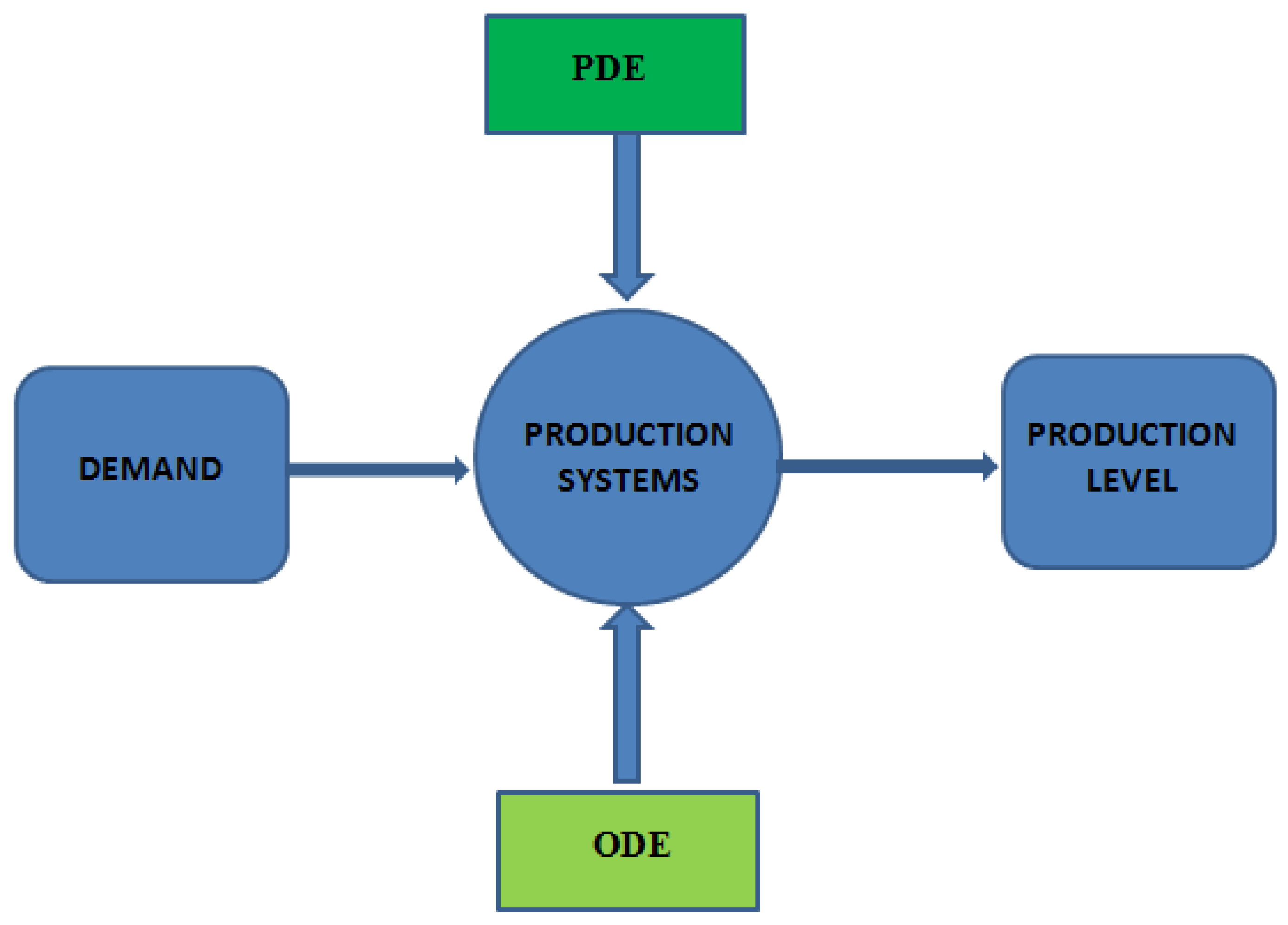
Figure 1 presents a general taxonomy for production systems, from a mathematical modeling context, considering the demand profile and production level along this research work.

This technical note is integrated in section 2 by the mathematical formulation and solution of the infinite dimensional system for production level modeling, in section 3, a finite dimensional production-inventory system is analyzed with a proper stability analysis. Finally, conclusions and future work are present in section 4.

2. Infinite dimensional production level modeling

In general, a production system combines humans, machinery and equipment that are next to common material and information flow [23]. In a previous work [24], a PDE for production level subject to dynamic pricing and time, was presented, with the form:

v_{p} \frac{\partial^{2} φ (p, t)}{\partial p \partial t} + (β + a_{p}) \frac{\partial φ (p, t)}{\partial p} + α β \frac{\partial φ (p, t)}{\partial t} + K φ (p, t) = D (p, t)

(1)

Where

φ (p, t)

is the production level subject to price and time,

D (p, t)

is the demand level, v_p is the price velocity, a_p is the price acceleration, β is the damping coefficient, α is the scaling production factor and K is the production system resilience, with

β + a_{p} > 0 .

Our aim is to solve equation (1) analytically, subject to similar conditions for which a production system approaches to demand levels near to zero.

Theorem 1.

Considering the PDE in (1) assumming that:

D (p, t) = w P^{’}

β + a_{p} = 1

and

α β = 1

, which gives the following solution:

φ (p, t) = e^{- α p} (e^{- (\frac{K - α}{1 - α v_{p}}) t} + \frac{α w}{α - K})

Proof.

v_{p} \frac{\partial^{2} φ (p, t)}{\partial p \partial t} + \frac{\partial φ (p, t)}{\partial p} + \frac{\partial φ (p, t)}{\partial t} + K φ (p, t) = w P^{’}

(2)

Applying the separation of variables method, we have the following:

φ (p, t) = P (p) T (t) .

(3)

Substituting equation (3) in the PDE (2):

\dot{v_{p} P^{'} T^{'} + P^{'} T - w P^{'} + P T^{'} + K P T = 0} .

(4)

Where:

P^{'} = \frac{d P}{d p}

and

T^{'} = \frac{d T}{d t}

Grouping terms from equation (4):

P^{'} (v_{p} T^{'} + T - w) = - P (T^{'} + K T) .

(5)

Separating terms in equation (5):

- \frac{P^{'}}{P} = \frac{(T^{'} + K T)}{v_{p} T^{'} + T - w} = α .

(6)

For separate ordinary differential equation (ODE), in time domain:

\frac{P^{'}}{P} = - α .

(7)

Therefore:

\frac{d P}{P} = - α d p .

(8)

Solving equation (8):

P (p) = e^{- α p} .

(9)

For the ODE, in time domain:

T^{'} + K T = α (v_{p} T^{'} + T - w) .

(10)

After some algebraic manipulation, equation (10) becomes:

T^{'} + (\frac{K - α}{1 - α v_{p}}) T = - (\frac{α w}{1 - α v_{p}}) .

(11)

Solving the equation (11), we have:

T (t) = C e^{- (\frac{K - α}{1 - α v_{p}}) t} + \frac{α w}{K - α} .

(12)

Finally, the solution for the PDE production level subject to price and time is:

φ (p, t) = e^{- α p} (e^{- (\frac{K - α}{1 - α v_{p}}) t} + \frac{α w}{α - K}) .

(13)

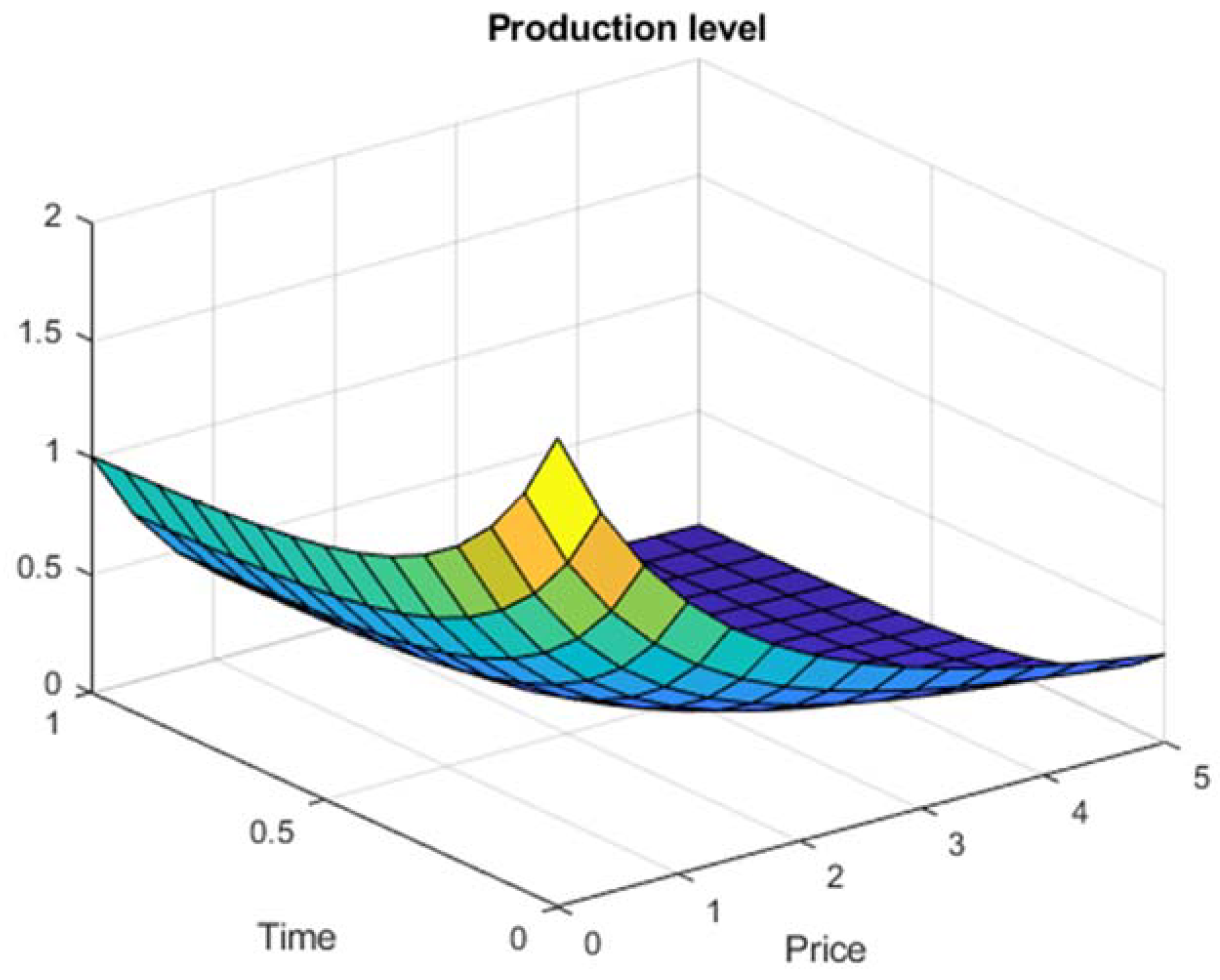
In Figure 2, a PDE production level normalized solution in function of price and time is present, considering a tendency to zero production level conforming price and time tends to infinity.

3. Finite dimensional production-inventory modeling

In [25] a dynamic production-inventory system is presented via optimal control theory. For mathematical modeling purposes an extension, of this previous work is present here, considering dynamic pricing and time delayed effects.

3.1. Mathematical modeling

A time-delayed production inventory system is proposed via a set of coupled ordinary differential equations which are described as follows: In order to incorporate a dynamic pricing perspective in the production-inventory system, we propose:

\frac{d p}{d t} = u_{1} (t) - p (t) + k \frac{I (t)}{C}

(14)

Where from equation (14),

u_{1}

= denotes the purchase price level; p = denote the sales price level; I= inventory level; k= associated cost for inventory and C=Capacity level.

To develop the production-inventory system dynamics for production level and production rates, the following equation is proposed:

C \frac{d^{2} Q}{d t^{2}} + I (t) \frac{d Q}{d t} + γ Q (t - θ) = d (t)

(15)

From equation (15), Q= production level; dQ/dt= production rate; d= demand level, θ= lead time and

γ

= production resilience factor.

The following ODE describes the inventory level of the system:

\frac{d I}{d t} = μ I (t - θ) + γ Q (t) - d (t)

(16)

In order to provide a linear approximation, via Taylor series, for the time delay terms as in [26], and neglecting high order terms:

x (t - τ) \approx x (t) - τ \dot{x} (t)

(17)

Developing a state space formulation for the time delayed production inventory system from equations (14)-(16) and applying equation (17) our new state space system is:

\dot{x_{1}} (t) = - x_{1} (t) + k_{1} x_{4} (t)

(18)

\dot{x_{2}} (t) = x_{3} (t)

(19)

\dot{x_{3}} (t) = - k_{2} x_{3} (t) x_{4} (t) - k_{3} x_{2} (t) + k_{4} x_{3} (t)

(20)

\dot{x_{4}} (t) = k_{5} x_{2} (t) + k_{6} x_{4} (t)

(21)

Where x₁(t) = p(t), x₂(t)=Q(t), x₃(t)=dQ/dt, x₄(t) = I(t) and the constants k₁ = k/C, k₂ = 1/C, k₃ =γ/C, k₄ = γθ/C, k₅ = γ/(1+μθ), k₆ = μ/(1+μθ).

3.2. Stability analysis

Theorem 2.

In order to have a stability analysis, for the system of equation 18-21, the following conditions must be satisfied,

γ ϑ > 0

μ > 0

and

C > 1 + μ θ

Proof.

In order to proof theorem 2, the following Lyapunov candidate function is proposed:

V (x_{1}, x_{2}, x_{3}, x_{4}) = \frac{1}{2} x_{1}^{2} + \frac{1}{2} x_{2}^{2} + \frac{1}{2} {(x_{3} - x_{4})}^{2}

(22)

Applying the derivative with respect to time, to the Lyapunov candidate function:

\dot{V} (x_{1}, x_{2}, x_{3}, x_{4}) = x_{1} {\dot{x}}_{1} + x_{2} {\dot{x}}_{2} + (x_{3} - x_{4}) ({\dot{x}}_{3} - {\dot{x}}_{4})

(23)

After some algebraic manipulation, and applying the LaSalle Theorem in the equilibrium point.

\dot{V} (x_{1}, x_{2}, x_{3}, x_{4}) < - x_{1}^{2} + k_{4} x_{3}^{2} + k_{6} x_{4}^{2} - (k_{3} - k_{5} - 1) {| Q |}^{2} - (k_{4} + k_{6}) {| O |}^{2} - (k_{5} - k_{3}) {| P |}^{2}

(24)

Equation 24, can be simplified to:

\dot{V} (x_{1}, x_{2}, x_{3}, x_{4}) < - x_{1}^{2} - (k_{4} + k_{6}) {| O |}^{2} - (k_{5} - k_{3}) {| P |}^{2}

(25)

In order to achieve stability, the following condition must be satisfied:

k_{4} + k_{6} > 0

k_{5} - k_{3} > 0

Therefore:

k_{4} > 0

and

k_{6} > 0

Considering that:

k_{4} = \frac{γ θ}{C}

and

k_{6} = \frac{μ}{1 + μ θ}

Also,

k_{5} > k_{3}

From which we can conclude that:

γ ϑ > 0 μ > 0 C > 1 + μ θ

3.3. Simulations

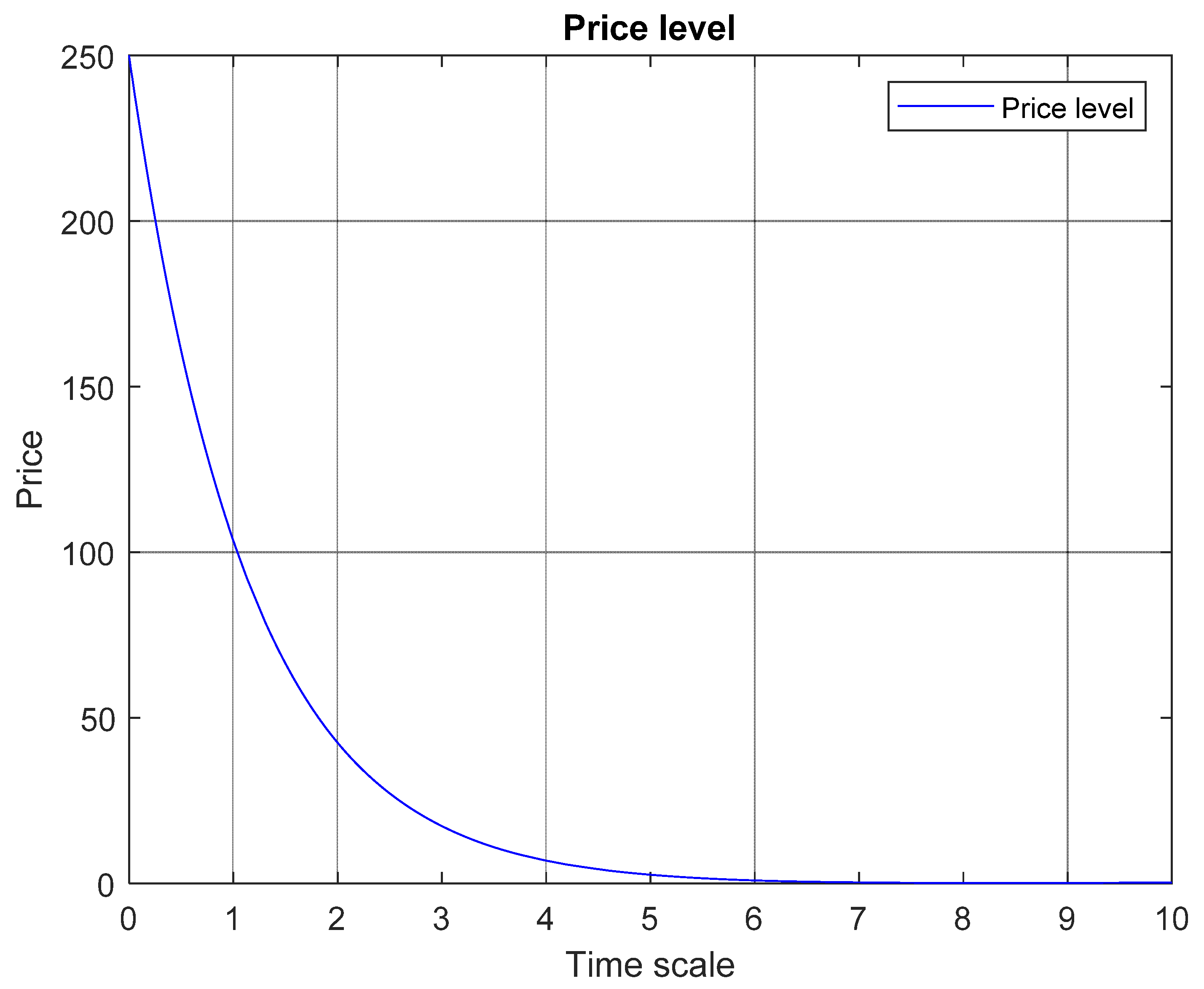
Simulations were developed applying MATLAB, for the equations (18)-(21), in which in Figure 3 presents a decaying performance for price level of the finite dimensional production system. This is considering the Equation 14, which presents the dynamic pricing analysis for production-inventory system. Conforme time increases the pricel level tends to zero.

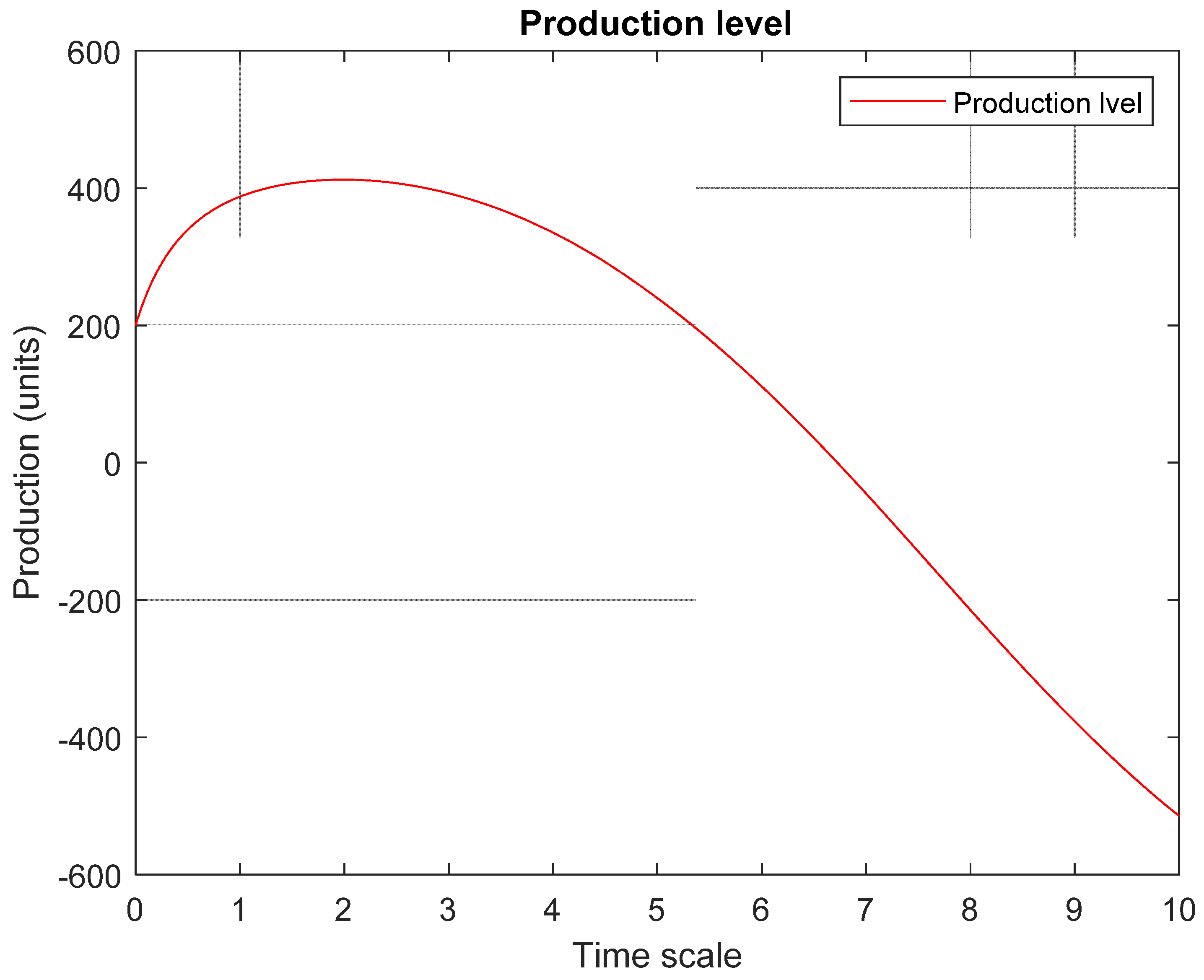
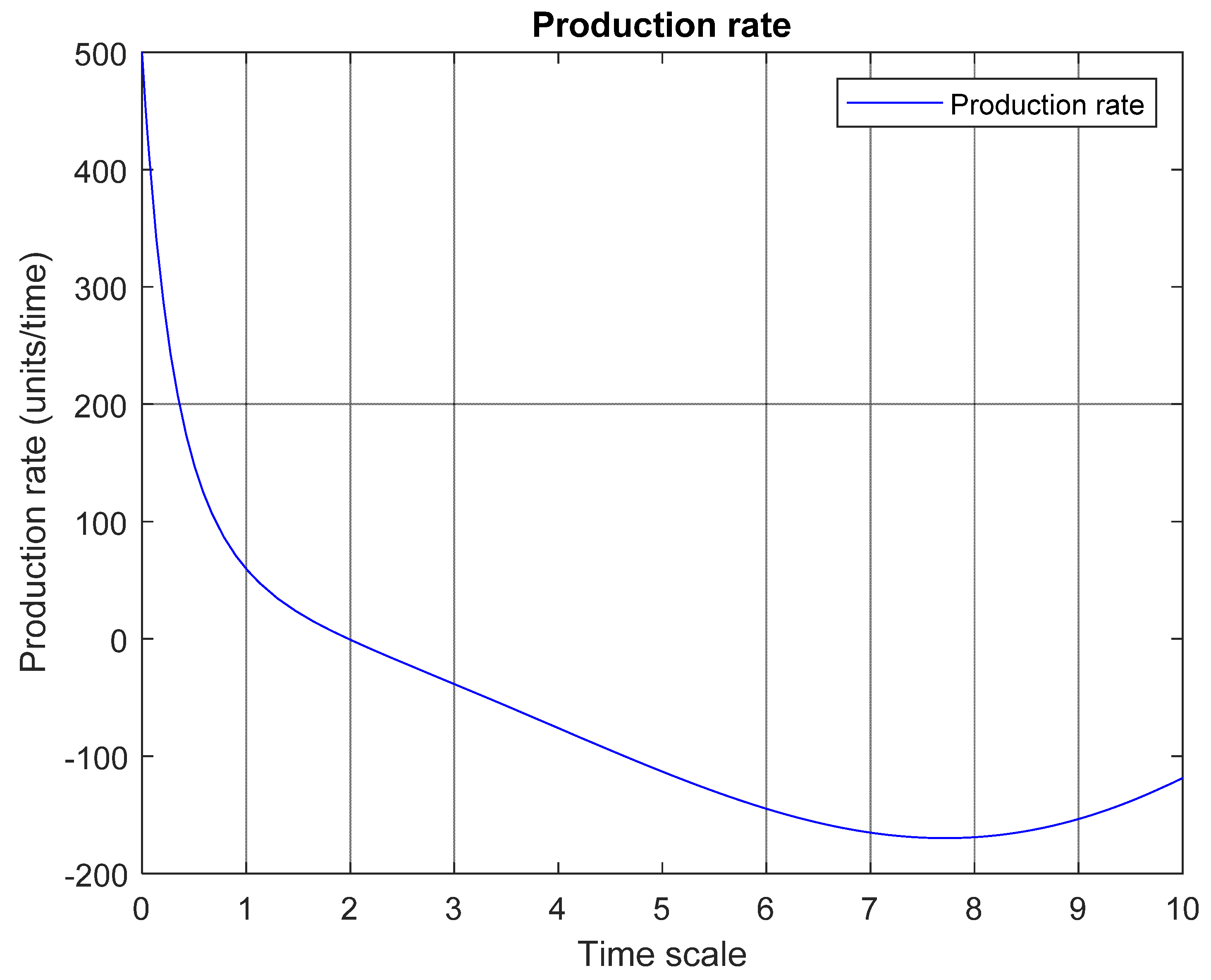
In Figure 4 a production level achieves a maximum for the finite dimensional system which is based on the context that this is the level the production rate. From Figure 5, unproduce is related with a negative production rate performance. This effect is present aroung time unit two, and conforms tends to higher values the production rate decreases.

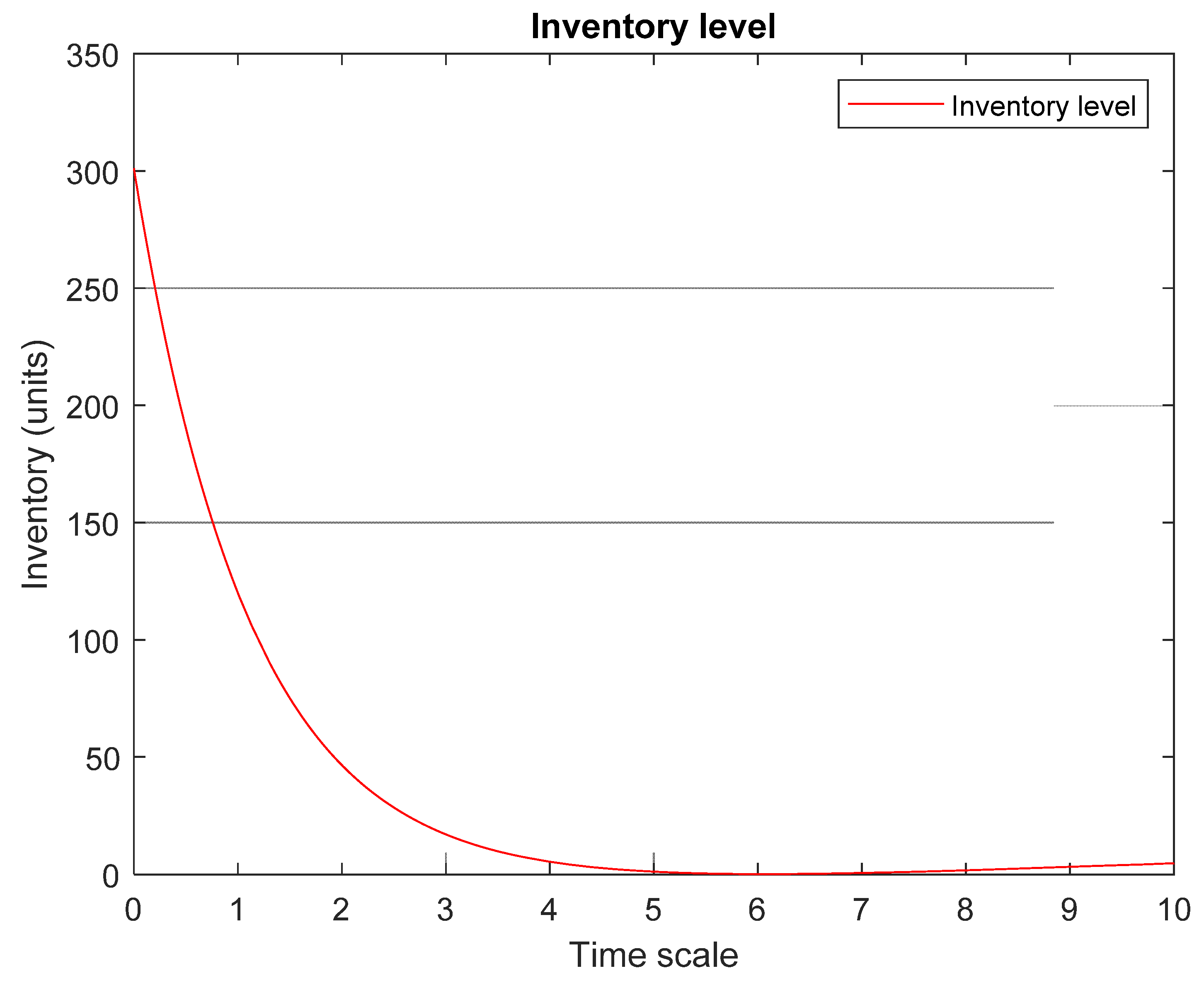
Figure 6 presents a decaying inventory level conforms production rate tends to a negative value, which is an effect of the relation of maximum production level towards lower levels for inventory. This is present from Equation 16, which presents a dynamic inventory level with time delaying.

4. Conclusions

This communication presents that mathematical modeling in high volume production systems, is important via the application of infinite and finite dimensional approaches, which corresponds to the use of partial differential equations (PDE) and ordinary differential equations (ODE), respectively.

This mathematical modeling considers low variability and cause-effect relation for deterministic approach in high volume production systems. This research work presents two novel approaches via PDE and ODE to model high volume production systems, with emphasis on demand fluctuation. In general, demand fluctuation corresponds to product demand variation, which is increased or decreased in a time horizon period.

In future work, our interest is to apply optimal control theory in order to extend the results based on mathematical modeling for both dynamical systems.

Author Contributions

Conceptualization, Y.Davizón, J.Amillano, and J. Leyva; methodology, C.Hernández, J.Sanchez and R. Ramírez; software, Y.Davizón and E. Olivares.; validation, B.Valenzuela and E.Smith ; formal analysis, C.Hernández and E. Olivares; investigation, Y.Davizón.; resources, B.Valenzuela, E. Olivares, R. Ramírez and N.Smith; writing—original draft preparation, Y.Davizón and J.Amillano; writing—review and editing, J.Sanchez, C.Hernández and J. Leyva; supervision, E. Olivares and E.Smith; funding acquisition, E.Olivares, J.Sanchez, E.Smith and N.Smith. All authors have read and agreed to the published version of the manuscript.

Funding

This research was funded by Universidad Panamericana (grant number UP-CI-2022-GDL-11-ING).

Acknowledgments

The authors are grateful and recognize the optimal feedback provided by Dr. Cesar Martínez-Olvera and Dr Carlos Hinojosa, for their comments and advising during the development of this research work.

Conflicts of Interest

The authors declare no conflict of interest.

References

Sourirajan, K. , Ramachandran, B. and An, L. Application of control theoretic principles to manage inventory replenishment in a supply chain. International Journal of Production Research. 2008. 46 (21). pp. 6163–6188.
Perea, E., Grossmann, I., Ydstie, E., and Tahmassebi, T. Dynamic modeling and classical control theory for supply chain management. 2000. Computers and Chemical Engineering 24 pp.1143-1149.
Dolgui, A. , Ivanov, D., Sethi, S. and Sokolov, B. Control theory applications to operations systems, supply chain management and Industry 4.0 networks. 2018. IFAC PapersOnLine 51-11 pp. 1536–1541.
Sucky, E. Inventory management in supply chains: A bargaining problem. International Journal of Production Economics. 2005. 93-94. pp. 253-262.
Sarimveis, H. , Patrinosa, P., Tarantilis, C.D. and Kiranoudisa, C.T. Dynamic modeling and control of supply chain systems: A review. 2008. Computers & Operations Research 35 pp. 3530–3561.
Singh, D. and Verma, A. Inventory management in supply chain. Materials Today: Proceedings 5 (2018) 3867–3872.
Bieniek, N. The ubiquitous nature of inventory: Vendor Managed Consignment Inventory in adverse market conditions. European Journal of Operational Research. 2019. In press.
Duan, L. and Ventura, J.A. A Dynamic Supplier Selection and Inventory Management Model for a Serial Supply Chain with a Novel Supplier Price Break Scheme and Flexible Time Periods. European Journal of Operational Research. (272) 2019.
Paul, S.K. , Sarker, R. and Essam, D. Managing risk and disruption in production-inventory and supply chain systems: A review. Journal of Industrial & Management Optimization, 2016, 12 (3). pp.1009-1029. [CrossRef]
Li, S. , He, Y. and Lujie, C. Dynamic strategies for supply disruptions in production-inventory systems. International Journal of Production Economics.2017, 194. pp 88-101. [CrossRef]
Pal, B. , Sana, S.S. and Chaudhuri, K. A multi-echelon production–inventory system with supply disruption. Journal of Manufacturing Systems. 2014, 33(2), pp. 262-276. [CrossRef]
He, Y. and He, J. A Production Model for Deteriorating Inventory Items with Production Disruptions. Discrete Dynamics in Nature and Society. 2010. Article ID 189017. [CrossRef]
Karim, R. and Nakade, K. A stochastic model of a production-inventory system with consideration of production disruption. International Journal of Advanced Operations Management, 2019. 11(4). pp.287- 316. [CrossRef]
Moinzadeh, K. and Aggarwal, P. Analysis of a Production/Inventory System Subject to Random Disruptions. Management Science, 1997. 43(11), pp.1577-1588. [CrossRef]
Sánchez-Ramírez, C. , Ramos-Hernández, R., Mendoza Fong, J.R., Alor-Hernández, G., and García-Alcaraz, J.L. A system dynamics model to evaluate the impact of production process disruption on order shipping. Applied Sciences, 2020, 10, 208. [CrossRef]
Stephens, A.R. , Kang, M. and Robb, C.A. Linking Supply Chain Disruption Orientation to Supply Chain Resilience and Market Performance with the Stimulus–Organism–Response Model. Journal of Risk and Financial Management. 2022.
Nunes, M. , Abreu, A. Bagnjuk, J., Nunes, E. and Saraiva, C. A Strategic Process to Manage Collaborative Risks in Supply Chain Networks (SCN) to Improve Resilience and Sustainability. Sustainability, 2022.
Morikawa, M. Demand fluctuations and productivity of service industries. Economics Letters. 2012.
Paul, S.K. , Sarker, R. and Essam, D. Managing real-time demand fluctuation under a supplier–retailer coordinated system. Int. J, Production Economics. 2014.
Tian, Z. , Zhou, J. and Wang, M. Dynamic evolution of demand fluctuation in bike-sharing systems for green travel. Journal of Cleaner Production, 2019.
Yang, L. , Ng, C.T. and Cheng, T.C.E. Optimal production strategy under demand fluctuations: Technology versus capacity. European Journal of Operational Research. 2011.
Xiong, G. and Helo, P. An application of cost-effective fuzzy inventory controller to counteract demand fluctuation caused by bullwhip effect, International Journal of Production Research, 2006.
Alexopoulos, K. , Papakostas N., Mourtzis D., Gogos, P. & Chryssolouris, G. Oscillator analogy for modelling the manufacturing systems dynamics, International Journal of Production Research, 2008, 46:10, 2547-2563.
Davizón, Y.A. , Soto, R., Rodríguez, J.J., Rodríguez-Leal, E., Martínez-Olvera, C. and Hinojosa, C. Demand management based on model predictive control techniques. Mathematical Problems in Engineering, 2014. Article ID 702642. [CrossRef]
Davizón, Y.A.; Martínez-Olvera, C.; Soto, R.; Hinojosa, C.; Espino-Román, P. Optimal Control Approaches to the Aggregate Production Planning Problem. Sustainability 2015, 7, 16324-16339. [CrossRef]
Insperger, T. On the Approximation of Delayed Systems by Taylor Series Expansion. Journal of Computational and Nonlinear Dynamics. 2015, Vol. 10.

Figure 1. General taxonomy for production systems

Figure 2. PDE production level solution in function of price and time

Figure 3. Price level for the finite dimensional production system

Figure 4. Production level for the finite dimensional production system

Figure 5. Production rate for the finite dimensional production system

Figure 6. Inventory level for finite dimensional production system

Table 1. Demand Fluctuation Literature review.

Paper	Contribution	Application
Morikawa [18]	The aim of this paper presents evidence on the relationship between short-term demand fluctuations and the total factor productivity of service industries.	Service industries
Paul, et al [19]	This paper considers a supplier–retailer system, with an imperfect production process and a possibility of having demand fluctuation. Also, a dynamic planning process is analyzed to deal with short-term demand fluctuations.	Supply chain

Tian, et al [20]	This paper main contribution is the statistical physics method is applied to the demand fluctuation of two different bike sharing system.	Urban traffic
Yang, et al [21]	This paper presents a comparison for two types of flexibility investment, which are flexible technology and flexible capacity, under demand fluctuations.	Flexible manufacturing systems
Xiong and Helo [22]	This paper presents a fuzzy inventory model to counteract the demand fluctuation in supply demand networks, applying fuzzy logic controller.	Supply demand networks

Disclaimer/Publisher’s Note: The statements, opinions and data contained in all publications are solely those of the individual author(s) and contributor(s) and not of MDPI and/or the editor(s). MDPI and/or the editor(s) disclaim responsibility for any injury to people or property resulting from any ideas, methods, instructions or products referred to in the content.

© 2023 by the authors. Licensee MDPI, Basel, Switzerland. This article is an open access article distributed under the terms and conditions of the Creative Commons Attribution (CC BY) license (https://creativecommons.org/licenses/by/4.0/).

Copyright: This open access article is published under a Creative Commons CC BY 4.0 license, which permit the free download, distribution, and reuse, provided that the author and preprint are cited in any reuse.

MDPI Initiatives

Important Links

Choose an area of interest and we will send you notifications of new preprints at your preferred frequency.

Disclaimer

Mathematical Modeling for Infinite and Finite Dimensional Production-Inventory Systems Subject to Demand Fluctuation

Abstract

1. Introduction

2. Infinite dimensional production level modeling

3. Finite dimensional production-inventory modeling

3.1. Mathematical modeling

3.2. Stability analysis

3.3. Simulations

4. Conclusions

Author Contributions

Funding

Acknowledgments

Conflicts of Interest

References

MDPI Initiatives

Important Links

Subscribe