Preprint
Article

Towards Automated Measurement of As-Built Components Using Computer Vision

Altmetrics

Downloads

103

Views

15

Comments

0

A peer-reviewed article of this preprint also exists.

This version is not peer-reviewed

Submitted:

28 July 2023

Posted:

01 August 2023

You are already at the latest version

Alerts
Abstract
Regular inspections during construction work verify that the work completed is consistent with the plans and specifications and ensure that it is within the planned time and budget. This requires frequent physical site observations to independently measure and verify the completion percentage of the construction progress performed over periods of time. The current computer vision-based (CV) techniques for the measurement of as-built elements, predominantly use 3D laser scanning or 3D Photogrammetry modelling to determine the geometrical properties of as-built elements on construction sites. Both techniques require data acquisition from several positions and angles to generate sufficient information about the element’s coordinates making the deployment of these techniques on dynamic construction project sites a challenging task. In this paper, we propose a pipeline for automating the measurement of as-built components using artificial intelligence (AI) and computer vision (CV) techniques. The pipeline requires a single image obtained with a stereo-camera system to measure the size of selected objects or as-built components. We demonstrate our approach by measuring the size of concrete walls and columns. The novelty of this work is attributed to the fully automated CV-based method for measuring any given element using a single image only. The proposed solution is suitable for use in measuring the sizes of as-built components of built assets. It has the potential to be further developed and integrated with BIM models for use on construction projects for progress monitoring.
Keywords: 
Subject: Computer Science and Mathematics  -   Artificial Intelligence and Machine Learning

1. Introduction

The accurate and up-to-date measurement of as-built components is essential for the design, construction, operation and maintenance of as-built assets. Additionally, the measurement of as-built components is an essential part of construction project management functions such as cost and schedule control, financial reporting, claims and productivity measurement. It is, therefore, considered to be one of the most crucial, yet challenging tasks facing site managers. Most current approaches are still predominately manual, time-consuming and error-prone. Site managers normally spend a significant amount of time measuring, recording and analysing as-built information [1,2,3]. The lack of accurate and up-to-date as-built information due to the laborious and manual data collection practices could lead to increased cost, delays, and poor project performance, which in turn, could reduce the ability to detect or manage the variability and uncertainty inherent in the project activities [4,5,6].
In recent years, however, the construction industry has been exploring various emerging technologies to support the visual inspection and progress monitoring of construction work [7]. The on-site application of these technologies has indeed demonstrated significant potential for digitising and automating the capturing, measuring, and reporting updates of the as-built components and project information [6,8].
One notable example of these technological tools for automating the measurement of as-built components is the use of computer vision (CV). CV is a digitisation process for determining project progress which combines computer science, architecture, construction engineering, and management disciplines. It takes visual media, such as photos, videos, or scans as inputs and produces decisions or other forms of representation as outputs [9].
The two most popular CV-based techniques for measuring the as-built components are laser-based scanning, and imaging-based Photogrammetry [4,8,11,12]. Three-dimensional (3D) laser scanning is used to generate 3D point clouds which are processed to enable the estimation of sizes and quantities of as-built components [13]. The imaging-based approach, on the other hand, emulates human visualisation to extract three-dimensional (3D) geometrical information about objects from two-dimensional (2D) inputs [14,15].
A fully automated CV-based method for measuring as-built components would comprise four main sub-processes; data acquisition, information retrieval and processing, measurement estimation, and finally producing valuable output[16,17,18,19]. Each of the four sub-processes involves different techniques to achieve the desired outputs with its own benefits and limitations [8,20].
Despite some studies having made significant strides in automating CV-based methods for as-built component measurement, at present, there are still no applications that are fully automated. This is due to two main reasons. Firstly, the technologies involved are still emerging and undergoing experimentation with only a few functional demonstrations available [21]. Secondly, existing studies tend not to address the four stages together but focus on the individual stages, such as 3D point cloud generation in data acquisition [22,23], and feature recognition in information retrieval and processing [24,25,26].
This study aims to address this research gap by developing a pipeline for a fully automated as-built component measurement approach using CV-based methods. The proposed pipeline can run in real-time and is intended to estimate the size of as-built components of built assets. The pipeline employs stereo camera techniques for data acquisition, machine learning, object detection and instance segmentation for information retrieval and processing of as-built elements, Green’s theorem [27] for measurement estimation of the size of object(s) under consideration and finally visualisation of the output as labelled images. To demonstrate our work, we have trained a neural network model on concrete walls and columns, but the same principles can be extended to cover other types of as-built components.
The rest of this paper is structured as follows: Section 2 provides a literature review of related previous studies, highlighting the existing research and theories relevant to the subject matter. Section 3 focuses on the instrumentation and materials used in this study, outlining the experimental setup and the tools employed for data collection. We delve into the methodology of geometric estimation, explaining the mathematical models and algorithms utilised to estimate the geometric properties of the as-built components of interest. Section 4 presents the results obtained from our experiments, including a detailed analysis and discussion. Finally, section 5 summarises the key findings and conclusions drawn from this study, highlighting the implications, significance, and limitations of our research.

2. Literature Review

The measurement of as-built components is an essential aspect of the design, construction, operation and maintenance of built assets. It is particularly a key function in the continuous monitoring and periodic updates of the actual work undertaken on a construction site and comparing it with the as-planned or expected progress [28,29,30] and identifying variations between the planned and actual progress, which are essential for schedule updating [31]. The most common CV-based method for undertaking spatial measurements of the actual work on construction sites is 3D laser scanning. During the process, the construction site is scanned from different angles and locations at different times to generate spatial data, which can then be used to estimate the quantities of work performed within the time interval considered between two successive scans. 3D laser scanning yields data in the form of 3D points, known as “point clouds” which are later displayed as images that can be viewed from different perspectives using specialised software systems [32,33]. Many researchers have proposed and demonstrated that the technology can be used to obtain 3D data on the actual progress of a project efficiently [34,35,36,37,38].
However, this method has certain limitations as 3D data can be obtained only on the as-built components that are located within the laser scanner’s range and field of view. Secondly, even components that are physically within the range of the scanner may still be blocked from view by various pieces of equipment and other obstacles located around the construction site resulting in an incomplete 3D data set obtained on a construction site. To overcome this problem, a group of researchers have proposed UAV-based 3D laser scanning methods [39,40,41,42,43,44,45,46,47]. The authors argued that this approach can provide visual and detailed progress information with good area coverage and views from human-inaccessible angles. UAV-based data acquisition, however, requires careful operation handling as it can pose potential safety hazards and cause distractions to workers on-site. UAVs also require accurate path planning to avoid obstruction which in the case of any sudden rotational motion or sharp angular movements can result in motion blur. They can also be affected by wind speeds and other environmental anomalies.
Aside from issues related to the acquisition approach, there are other limitations associated with 3D laser scanning. This includes the time required to perform a single scan, and the number of scan positions necessary to acquire accurate information. The technique is also costly, technically intricate, and requires skilled experts to capture and model the whole project. Moreover, the collected 3D point cloud also requires extensive time and computational resources to process data and produce meaningful interpretations which may not be adequate for use on complex project sites to generate real-time updates.[48]. The incomplete or partially occluded patches in a 3D point cloud will also incur technical challenges during the registration of multiple point clouds [23,49,50,51].
On the other hand, the availability of high-quality and precise still image cameras has advanced 3D modelling from photo images [52]. As a result, an image-based scanning method called Photogrammetry has been proposed as an alternative to 3D laser scanning [53]. With Photogrammetry, the geometrical properties of an object on site are generated from its photo image. The technique, however, requires the placement of many targets strategically on the object(s) being photographed to identify the object’s coordinates and several photos of the object are then taken from different positions and angles to generate sufficient information on object coordinates [54]. The use of image-based scanning may also incur other practical limitations, particularly, when extracting geometrical properties of surfaces with little texture or poor definition [55]. Additionally, a recent study has also shown that the accuracy of the model generated from the image-based reconstruction is less than the laser scanner and becomes even less accurate as the length of the element increases. According to the study, the process of reconstructing a 3D model from an image dataset remains reliant on human intervention at various steps to improve the output quality.[56].
Compared to existing Photogrammetry techniques which require the placement of many targets on the object and several photos taken from different positions and angles to generate sufficient geometrical information, our proposed method requires a single image obtained from a stereo camera system and one target only to extract the information about the object’s coordinates. Additionally, unlike 3D laser-based scanning which also requires the construction site to be scanned from different locations and generates computationally extensive 3D point clouds, our proposed pipeline is capable of generating real-time updates of as-built components on construction sites.

3. Instrumentation

In this section, we discuss the pipeline for the full CV-based method which we have developed for measuring as-built components. To demonstrate our results, we used images containing concrete walls and columns captured from buildings at Oxford Brookes University - Headington campus to apply the pipeline to estimate the sizes and area of concrete elements. The pipeline which is depicted in Figure 1, can run in real-time and comprises seven steps: camera calibration, scene capturing, calculating the distance to a point in the scene, instance segmentation, depth map generation, estimate world coordinates, and finally calculating the area of the object of interest. This section will be divided into four subsections: data acquisition; information retrieval and processing; as-built component measurement; and finally visualisation of the output.

3.1. Initialisation

Camera calibration: We use a stereo camera system to capture the scene containing the object of interest. It is important that the camera system is accurately calibrated. The calibration is a one-time process for determining the intrinsic (principle point, distortion parameters, and focal length) and the extrinsic parameters (rotation and translation) of each camera and the relative pose between them. Both these sets of parameters are essential to attain 3D information given a set of 2D coordinates of corresponding image points. [57]. The process of recovering the third missing dimension is an ill-posed problem and is known in image geometry applications as depth estimation [58,59].
There are many different techniques for approximating the intrinsic and extrinsic parameters for a specific camera model. The most common one is Zhang’s method [60], (the one adopted in this work) and the direct linear transformation (DLT) [61].
Zhang’s method uses multiple views of a 3D pattern of known structure but unknown position and orientation in space. It is a flexible technique for camera calibration and well suited for use without specialised knowledge of 3D geometry or computer vision. The technique only requires the camera to observe a planar pattern shown at a few (at least two) different orientations. During the calibration process, both the camera and the planar pattern can be freely moved, but motion need not be known [60,62].
DLT on the other hand is a mathematical approach which aims to solve the problem of determining the pinhole camera parameters from at least six correspondences between 2D image points and 3D world points. A camera model maps each point of the 3D world to a point of the 2D image through a projection operation. The pinhole camera model makes the assumption that the aperture size of the camera is small so that it can be considered as a point. Thus, the ray of light has to pass across a single point, the camera centre and there are no lenses, no distortion, and an infinite depth of field [63,64].
In their simplest form, the intrinsic parameters can be represented by a 3 × 3 matrix called camera matrix denoted by the letter K as presented below:
K = f x 0 c x 0 f y c y 0 0 1
where f x , f y are the length of the focal point (in pixels) which is the distance from the centre of the lens to the principal points of the lens. c x , c y are the principal point which is the point on the image where a ray of light travelling perpendicular to the image plane passes through the focal point of the lens and intersects the camera’s sensor.

3.2. Data Acquisition

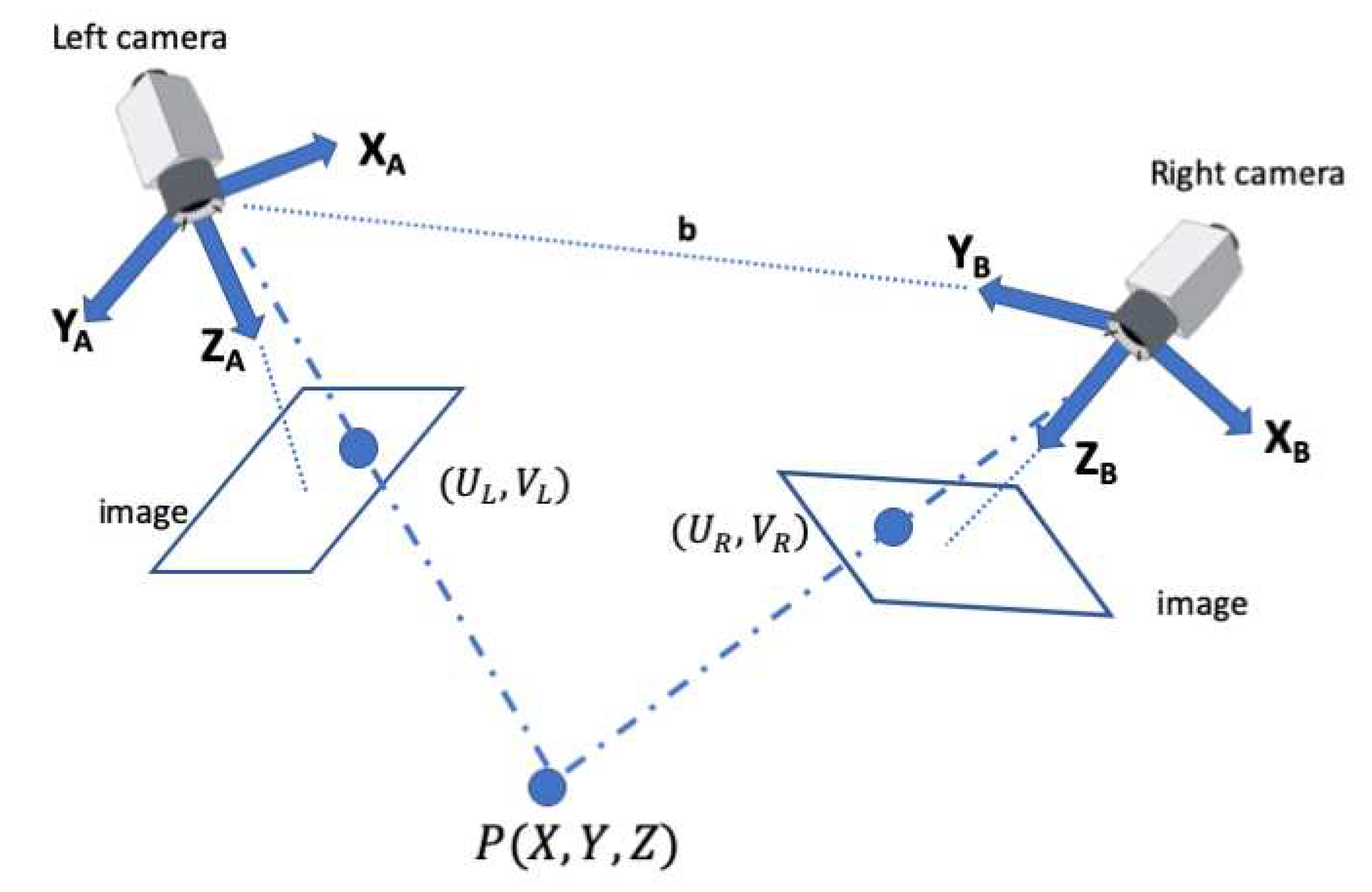
Scene capturing: A stereo vision system, also known as binocular stereo-vision, is a machine vision technique which uses exactly two cameras to capture a scene from two viewpoints. The two cameras are separated by a short distance known as the baseline b and are mounted almost parallel to one another. The principle of stereo vision is similar to that of the 3D perception of the human eyes. It can provide a 3D perception with real-time depth measurement based on the triangulation of rays from the two viewpoints (see Figure 2).
where b is the baseline, f is the focal length of the camera, u L and u R are the projections of the real-world point P in an image acquired by the left and right cameras. X A and Z A are the X-axis and the optical axis of the left camera respectively, whereas X B and Z B are the X-axis and the optical axis of the right camera respectively. P is a real-world point defined by the coordinates X, Y, and Z [65].
Calculating the distance to target (Z): In order to calculate the depth information Z, which is the distance to the real-world point P, first we need to calculate the disparity D which is the horizontal shift in position between two corresponding points projected on the image plane in the stereo vision system. In our approach, we used a red circular target and calculated the horizontal disparity between the centres of the circles appearing in the left and right frames. It is important that both the target and the object of interest are visible in the two frames, and that both the left and the right frames have at least 30 % overlapping. The calculation of the depth and disparity values are shown in (2), (3).
D = u L u R
Z = f b / D
where b is the baseline, f is the focal length of camera obtained from (1), u L and u R are the projections of the real-world point P in an image acquired by the left and right cameras [66].
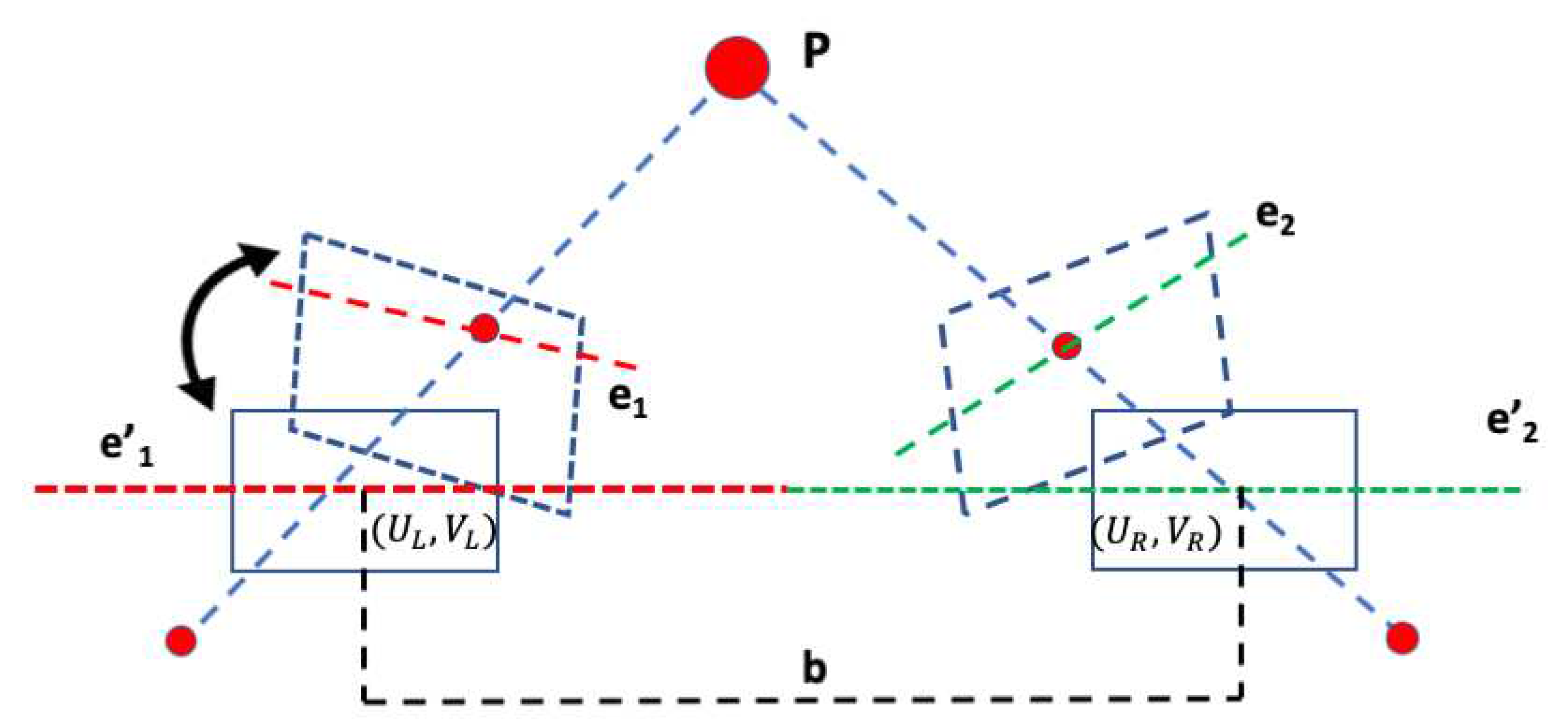
When capturing a scene from two distinct viewpoints using a stereo-cameras system, the left and right frames are not lined-up perfectly, and when the cameras rotate or move forward or backwards, the pixels will also move accordingly. This makes matching the corresponding pixels in each frame a very challenging task. To simplify the subsequent stereo correspondence problem, a process called rectification is applied first (see Figure 3). Stereo rectification is the determination of two image transformations (or homographies) that map corresponding points on the two images, projections of the same point in the 3D space, onto the same horizontal line in the transformed images [67,68].
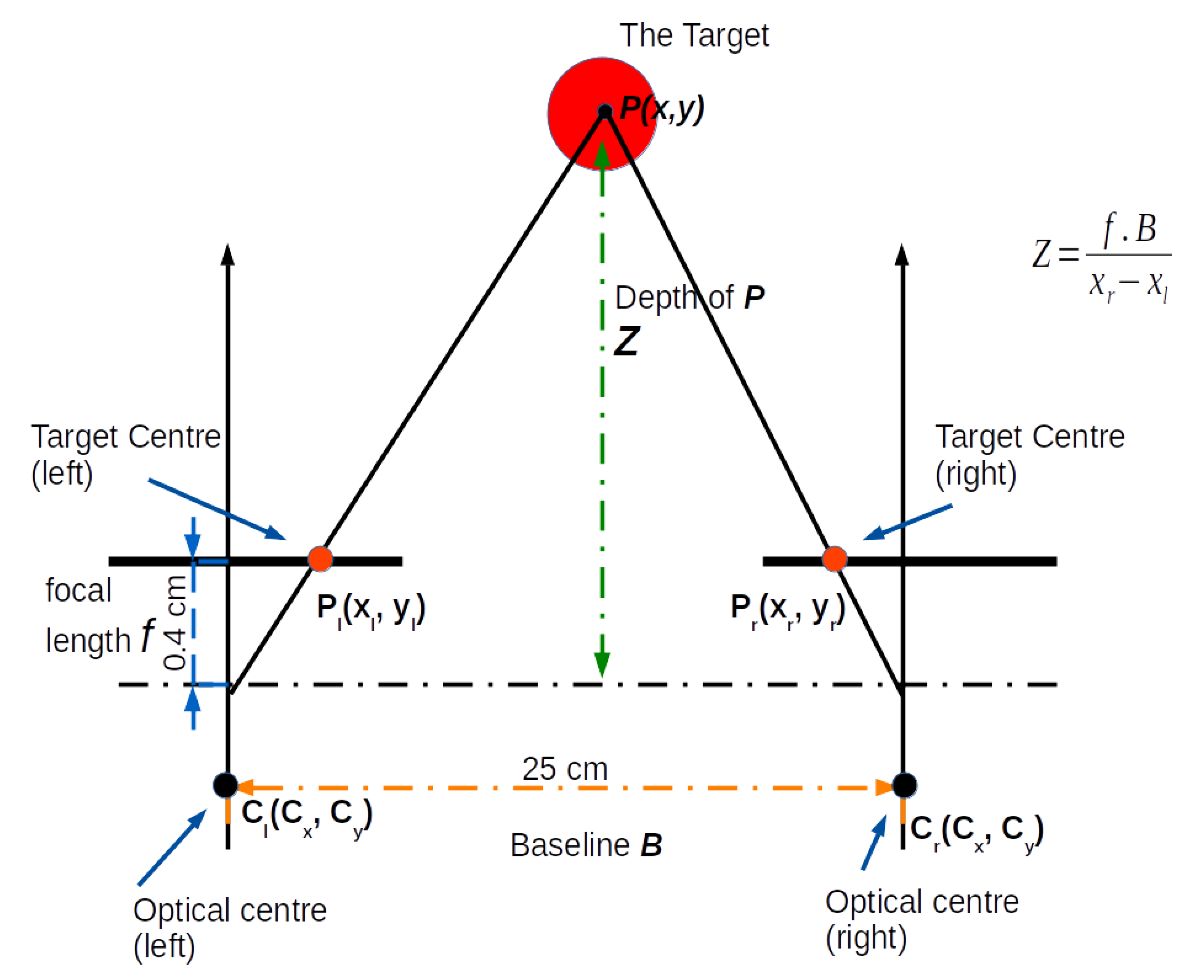
The target can be placed anywhere in the scene and need only to be visible by both cameras. Placing the target closer or on the object of interest would, however, improve accuracy. A target is any artefact object that can be distinguished from the surrounding, either by shape or colour. We used a red circular object as our target to be able to apply image processing techniques to detect the (red) colour and determine the circumference of the target in both left and right frames. The circular shape allows us to easily obtain the centre of the disk in both frames. Therefore, the horizontal displacement (the disparity D) between the two centres in the left and right frame is the difference between the x components of the target’s centre point ( x L x R ). To calculate the depth (i.e. the distance to target (Z) We apply the triangulation method (see Figure 9) to estimate the absolute distance to the target using (2 - 3).
Depth map generation: Depth estimation to all corresponding points projected on the image plane in the stereo vision system using the triangulation method will, inevitably, generate depth maps that are, in most cases, rough and sparse wherever matching between corresponding pixels fails [69]. Meanwhile, with the rapid development of deep/convolutional neural networks (CNN), monocular depth estimation based on deep learning has been widely studied recently and achieved promising performance in accuracy. These CNN-based methods are able to generate dense depth maps from single images where the depth at every pixel in the image is estimated by the neural network in an end-to-end manner [70,71,72] (see Figure 4). With CNN-based methods, the estimation of absolute depths (i.e. depth from the object to the camera) directly from a single image can be ambiguous in scale; for example, an object may appear the same as another identically-shaped but a smaller object in a nearer distance [73]. Relative depth on the other hand, which is the ratio between the depths of two points in an image is scale-invariant. This principle also applied to humans since it is easier even to choose the nearer between two points than to estimate the absolute depth of each point and therefore, relative depths are easier to estimate than ordinary (absolute) depths [73]. The adopted monocular depth estimation in this work [74] generates a relative dense depth map of each pixel in a single image with values between 0 and 1.0 where pixels with higher values are closer to the camera, and pixels with small values are further from the camera. By inverting this dense map we are able to assign small relative distances to closer pixels to the camera and higher relative distances to the furthest pixels from the camera.
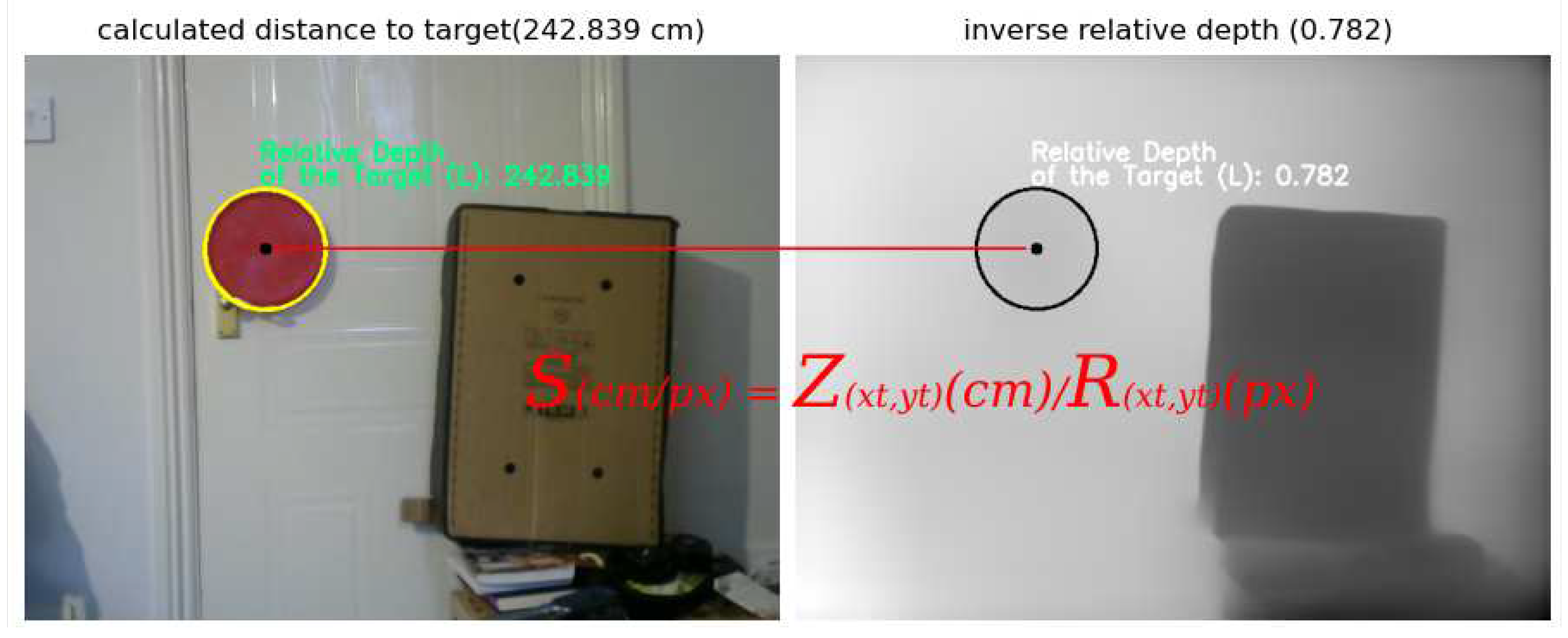
Next, we use the (absolute) distance of the target obtained from (2), (3) to compute a scalar S such that:
S c m / p x = Z x t , y t ( c m ) R x t , y t ( p x )
where Z x t , y t is the (absolute) distance to the centre of the target in cm, R x t , y t is the (relative) distance to the centre of the target in pixels (see Figure 5).
In this scenario, the scale S = 242.839 / 0.782 = 342.857 . By multiplying the scalar S with every entry in the relative dense depth map, we are able to generate the absolute depth map. To illustrate this, suppose a point p i is a pixel anywhere in the image with relative distance equal to the one for the centre of the target R x i , y j = 0.782 , i.e, both the point p i and the centre of the target are the same distance from the camera, then the absolute distance at p i = 0.782 × 342.857 = 242.389 cm, that is the same absolute distance of the target from the camera. Similarly, if p j is a pixel with relative distance R x i , y j = 0.384 , that is closer to the camera than the target, then the real distance of that point is p j = 0.384 × 342.857 = 130 cm.

3.3. Information Retrieval and Processing

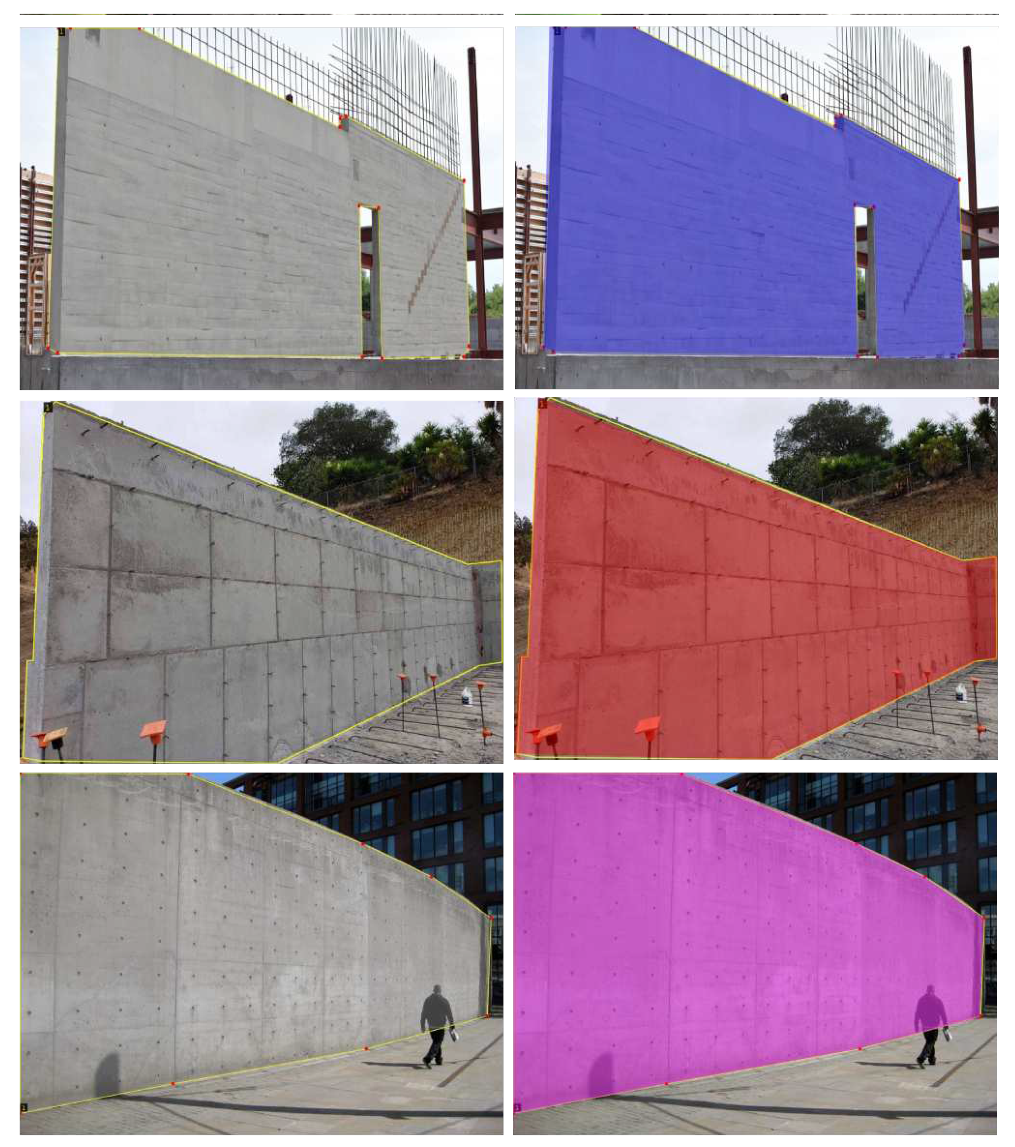
Instance Segmentation: Now, we turn our attention to Information retrieval and processing using object detection. Since our current implementation is devoted to measuring concrete structures (concrete columns and walls) only, we trained a neural network model [76] to extract (segment) those objects from a given image. A sample of the dataset used for training our model is presented in Figure 6).
Object detection and segmentation is the process of identifying the presence of an object in the image. It associates every pixel of that object with a single class label, e.g., a person, box, car and so on [77]. For every class, the neural network applies a unique colour mask over all the pixels of that object. There are two types of object segmentation, semantic: where the neural network treats multiple objects of the same class as a single entity and instance segmentation, which, in contrast to semantic, it treats multiple objects of the same class as distinct individual instances [77].
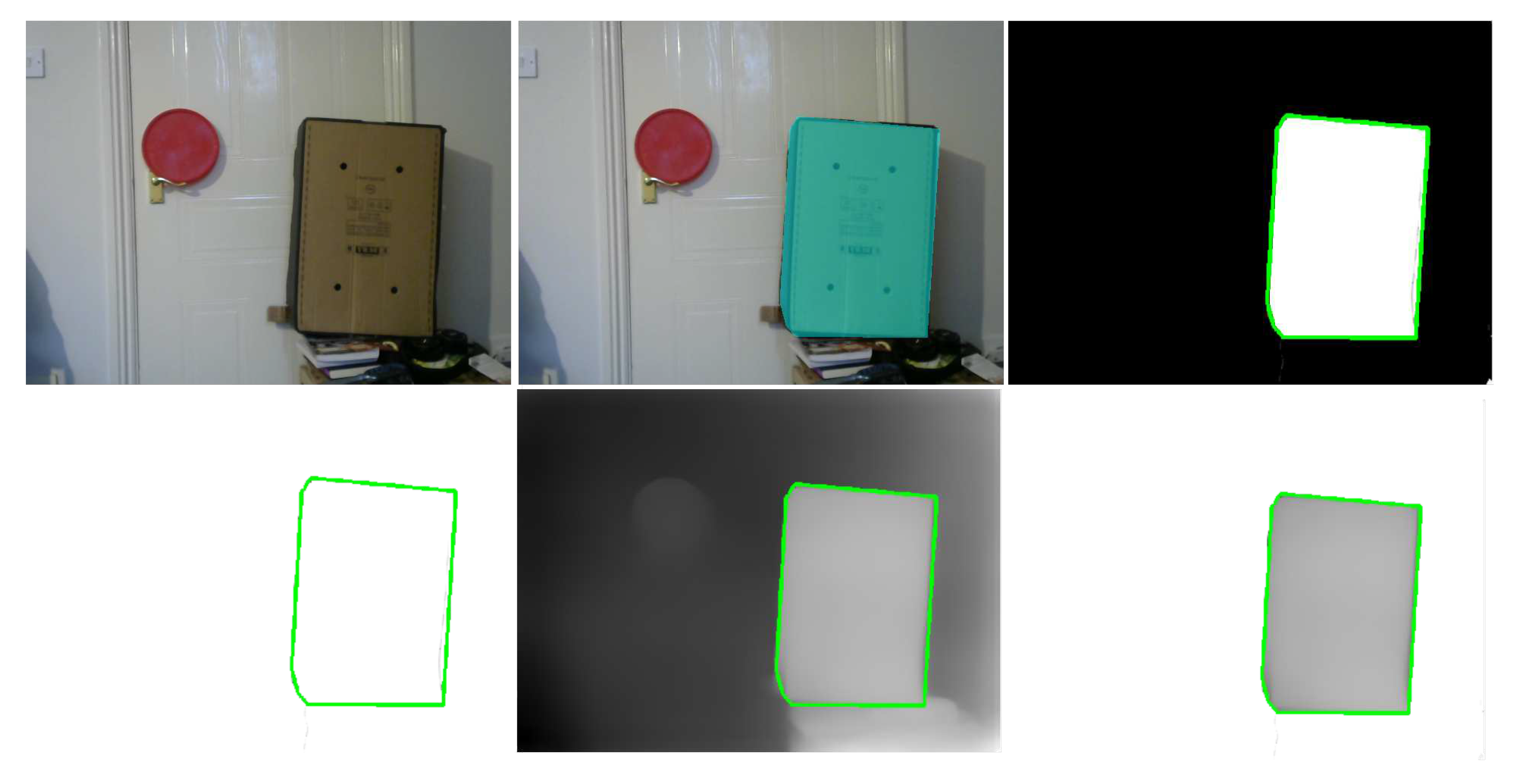
Figure 7 demonstrates the process of using object segmentation in an image to extract the corresponding pixels with absolute depth values of that object from the dense depth map.
First, we pass a single image (left frame) through the neural network for instance segmentation (Figure 7, top left). The model generates a colour mask over the object of interest and assigns all pixels related to the object with a single label (Figure 7, top middle). The corresponding masks of each object which are saved separately are used to extract the boundary of that object (Figure 7, top right).
The extracted boundary of the object (Figure 7, bottom left) is projected on the dense depth map containing the computed absolute depths (Figure 7, bottom middle) to separate only those pixels of the object of interest (Figure 7, bottom right). The mathematical formulation of this process is presented in the next section.

3.4. As-Built Component Measurement

Estimate world coordinates The next step of our proposed pipeline is to compute the real-world coordinates of the object and estimate the area of the object. The conversion to a real-world coordinate system (in cm) from the image-coordinate system (in pixels) is governed by the following equations:
X w = ( x c x ) Z x i , y j / f x
Y w = ( y c y ) Z x i , y j / f y
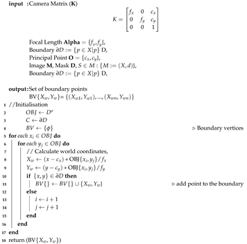
X w , Y w are the computed 2-dimensional real-world coordinates of each pixel in the object. x, y are the coordinates of each pixel in the object, c x , c y are the principal coordinates of the camera which are estimated during the calibration, f x , f y are the length of the focal point (in pixels) also found from the camera matrix (K), and Z x i , y j is the absolute distance at that pixel. The code in Algorithm 1 illustrates the procedure of obtaining the real-world coordinates of the object of interest.
Calculating the area of the object of interest: Lastly, we applied Green’s theorem [27] to calculate the area of the 2-dimensional irregular region, that is; the closure D ¯ which is enclosed by the boundary D and denoted in Algorithm 1 as B V .
Algorithm 1: Real World Coordinates
Preprints 80859 i001

3.5. Visualisation of the Output

The proposed pipeline which was entirely developed in Python can produce an output of any text or graphical format. This makes the integration of such output with any BIM model an easy task. Full demonstration of output samples is presented in Figure 10, Figure 11, Figure 13

4. Results and Discussion

We discuss our results through two examples; one for measuring a concrete column and the other example is for measuring a concrete wall at an Oxford Brookes University building. The building is a new addition to Oxford Brookes University and is mainly built from concrete components.
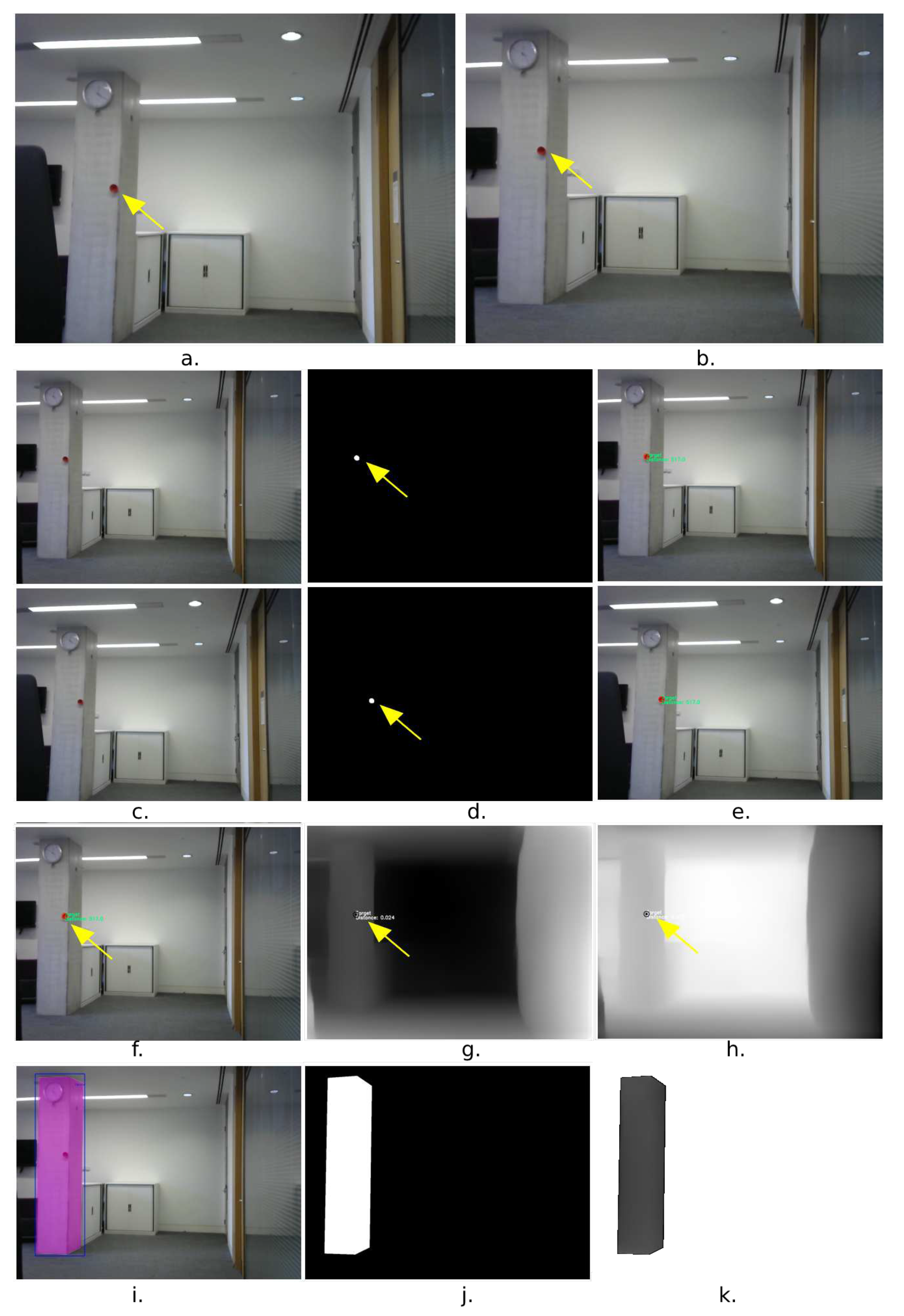
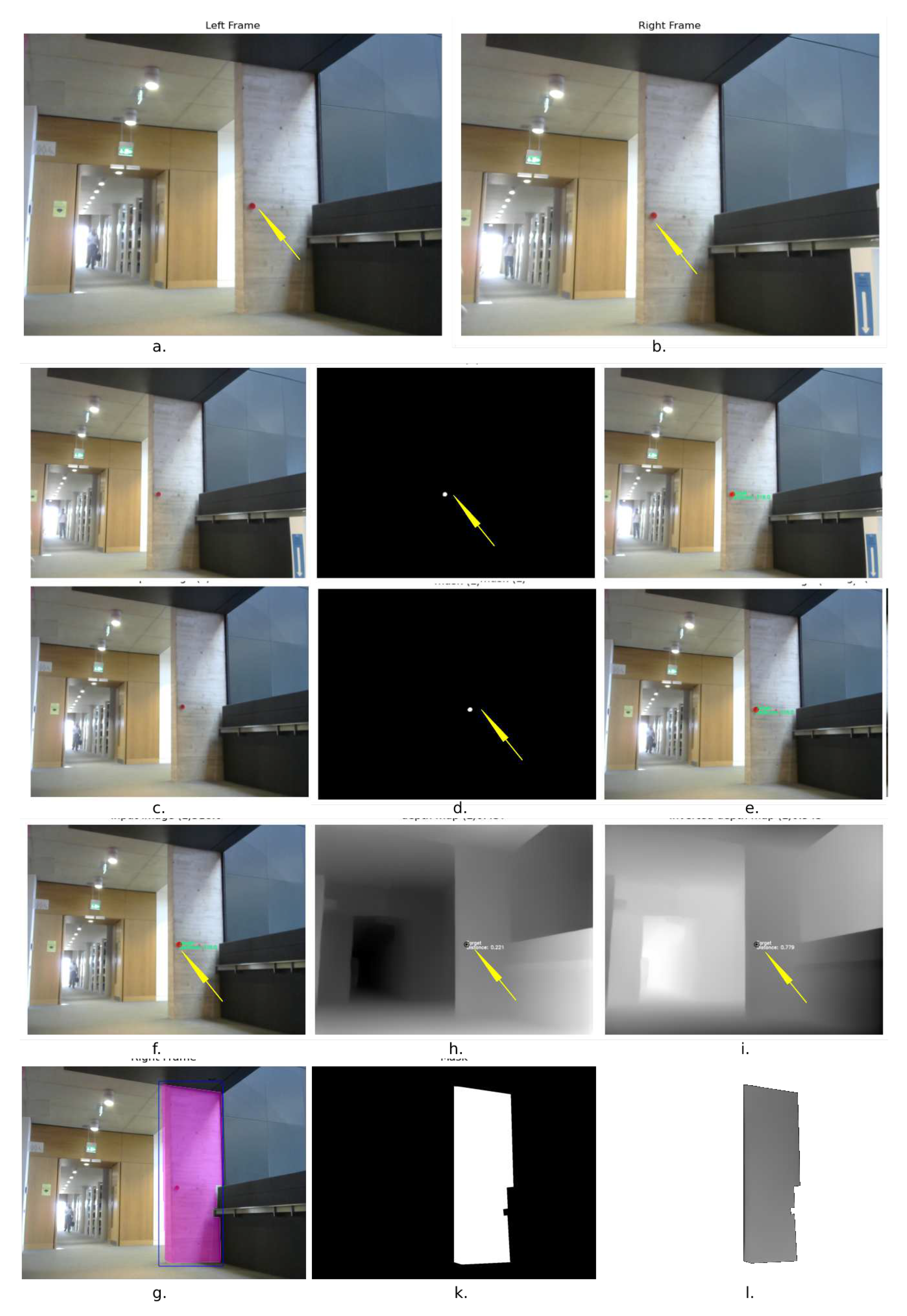
In the first experiment, we used a stereo camera system with baseline ( b = 25 cm) to capture the left and right frames of the scene. The stereo camera system was placed at a distance of 5.2m away from the column. The distance and the angle of the acquisition were chosen randomly but allowing the whole object (a concrete column) to appear completely in both frames. A target (red circular disk) was placed on the object at the same level of the stereo system where it is also visible in both cameras (Figure 8, a & b).
Once the scene was captured, a (red) colour filter was applied to allocate the target in both frames and calculate the coordinates of the centre of the circle in the left frame ( x l , y l ) (Figure 8, d-top row) and in the right frame (Figure 8, d-bottom row) ( x r , y r ) respectively. Next, using the principles of triangulation demonstrated in Figure 9, we calculated the depth Z x t , y t (e.g distance to the centre of the target) using the following formula:
Z x t , y t = f · B X r X l
where f is the horizontal focal length (in pixels), B is the baseline, and x r x l is the horizontal disparity. In this experiment, the calculated depth Z x t , y t to the centre of the target was 5.17m and the result was displayed on the left frame(Figure 8, e-top row) and on the right frame (Figure 8, e-bottom row) respectively.
Figure 8. Experiment 1
Preprints 80859 g008
Figure 9. Depth from disparity: P(x,y) is the real-world coordinates of the target centre, Z is the calculated distance (Depth) to the centre of the target. P l and P r represent the coordinates of the centre of the target in the left and right images respectively. C l and C r represents the principal points of the left and right cameras estimated during the calibration stage.
Preprints 80859 g009
We then passed the left frame (Figure 8, f) through our CNN-based monocular depth estimation model to generate the inverse dense depth map containing the relative depths of the scene (Figure 8, g). The dense depth map was then inverted again so that small relative depth indicates the closer points and the larger values refer to the further points (Figure 8, h).
To calculate the scalar S for this experiment, we use Z x t , y t = 517 c m , and R x t , y t = 0.976 , which is the relative depth value obtained from the inverted depth map (Figure 8, h) at the point x t , y t i.e, the centre of the target.
The scalar S is a case dependant, i.e. it varies depending on the position of the target in that scene. For this case, the scalar S is calculated as follows:
S = D c m R p x = 512 0.976 = 529.713 cm / px .
Now we multiply the inverted depth map shown in Figure (8h) by the scalar S to generate a dense map with absolute depths.
To extract the object (the concrete column) from the scene, we passed the left frame through our trained module for object detection and instance segmentation as shown in Figure (8, i). The output mask which is shown in Figure (8j) and corresponding to the detected object, i.e, the concrete column, is projected on the dense map with the absolute depth values which were generated in the previous step to extract only those segmented pixels related to the concrete column. Finally, we apply the code in Algorithm 1 the split the vertices belonging to the boundary ( B V ) and then use Green’s theorem to estimate the area of the concrete column.
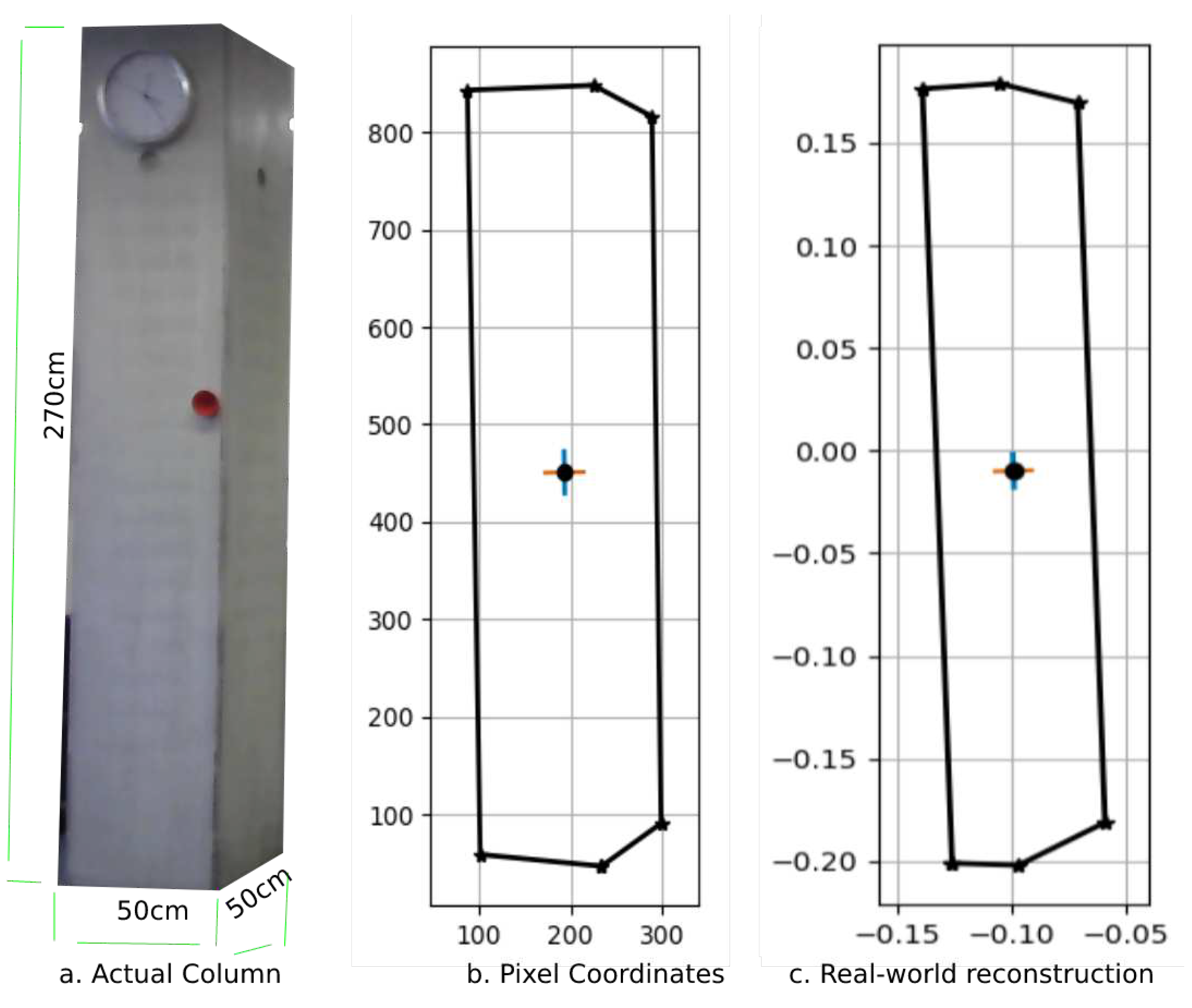
Figure 10. Real-world reconstruction of the concrete column.
Preprints 80859 g010
The actual surface area of the column, as shown in Figure 10a, is 270 c m ( h ) × 50 c m ( w ) = 1.35 m 2 × 2 faces = 2.70 m 2 . The pixel coordinates are shown in 10b are those of the mask generated during the instance segmentation process, and used to calculate the real-world reconstruction of the column 10c. The calculated surface area of the column is A = 2.5104 m 2 . The area of the front face (Figure 11b) is A = 1.1898 m 2 , and the area of the side face is A = 1.32055 m 2 . (Figure 11c)
Figure 11. Reconstructed Concrete Column.
Preprints 80859 g011
In the second experiment, we used the same stereo camera system with baseline ( b = 25 cm) to capture the left and right frames of the scene containing a section of concrete wall as depicted in Figure 12a, b. The stereo cameras system was placed at a distance of 5.6 m away from the wall section with the target placed also at the same level of the stereo system where it is visible by both cameras (Figure 12a & b).
In this experiment, the calculated depth Z x t , y t to the centre of the target was 5.59 m corresponding to R x t , y t = 0.779 . Therefore, the scalar S in this case is:
S = 559 0.779 = 717.586 cm / px .
Similarly, we multiply the inverted depth map shown in Figure (12h) by the scalar S to generate a dense map with absolute depths and then passed the left frame through our trained module for object detection and instance segmentation to extract the concrete wall section as shown in Figure (12i). The output mask which is shown in Figure (12j) and corresponding to the detected object, i.e, the concrete wall, is projected on the dense map with the absolute depth values which were generated in the respective step of the first experiment to extract only those segmented pixels related to the concrete wall. Finally, we apply the code in Algorithm 1 the split the vertices belonging to the boundary ( B V ) and then use Green’s theorem to estimate the area of the concrete wall.
Figure 13. Real-world reconstruction of the concrete wall.
Preprints 80859 g013
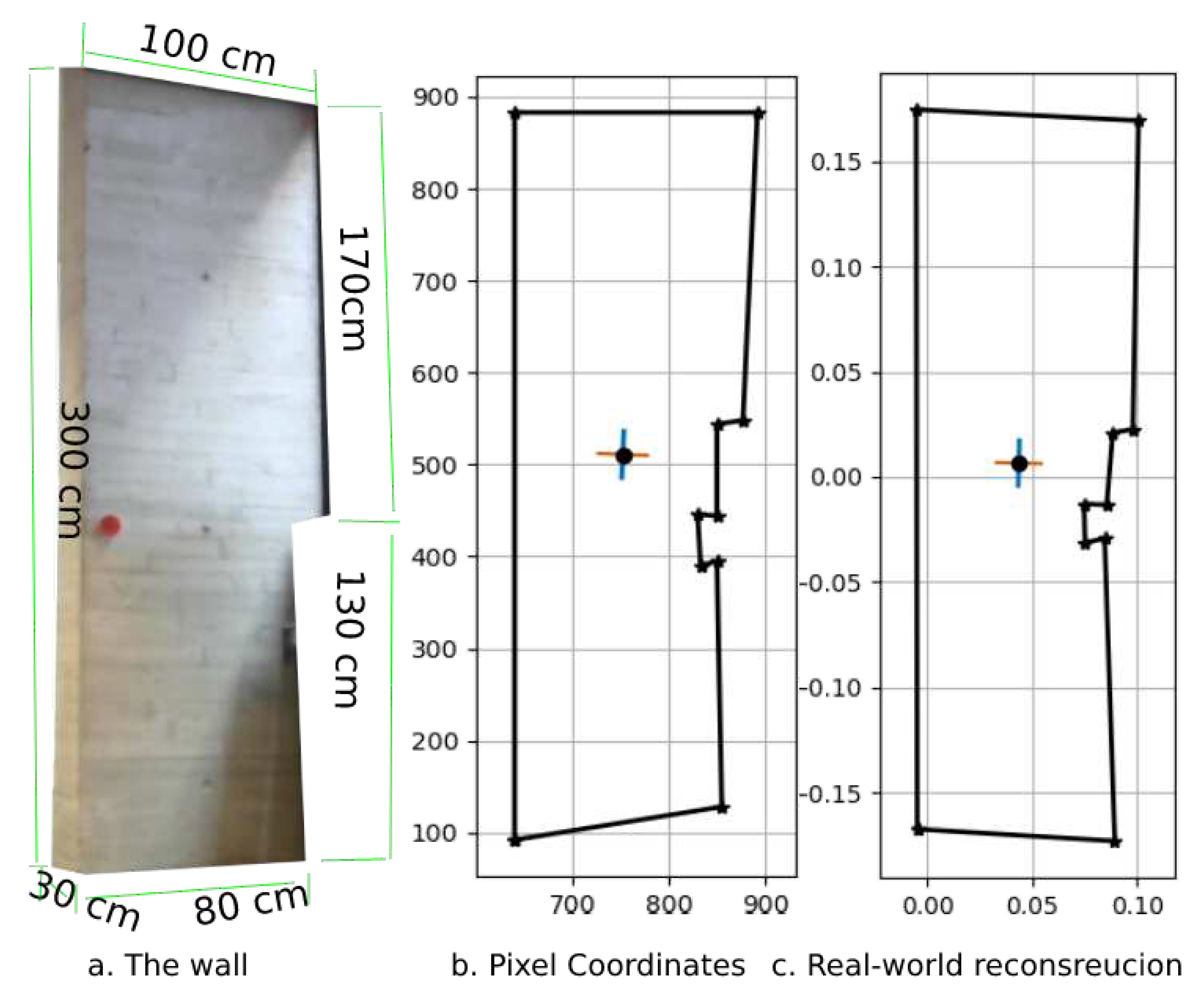
The actual surface area of the wall section is slightly more complex, it is the sum of the bottom half, the upper half and the side face as shown in Figure 13a : ( 130 c m × 80 c m ) + ( 170 c m × 100 c m ) + ( 30 c m × 300 c m ) = 36400 c m 2 or 3.64 m 2 . The pixel coordinates shown in 13b refer to the mask generated during the instance segmentation process and are used to calculate the real-world reconstruction of the column 13c. The calculated surface area of the column is A = 3.3143 m 2
The side face in this reconstruction is undetected therefore it is hard to estimate its contribution to the total estimated area.

4.1. Limitations

Inferring the depth from a two-dimensional image is known to be an extremely ill-posed problem. Errors may arise from many sources, but most importantly, the key contribution is attributed to the small scale at which the calculations are performed; i.e. the pixel scale, which will eventually be transformed to real-world scale; i.e. meters, cm, feet, or inches.
The first source of error comes from the camera calibration which is the process of estimating intrinsic and/or extrinsic parameters of the camera. During this process, we attempt to estimate the focal length of the camera in pixels; that is the distance between the lens and the image sensor when the subject is in focus and the principal point of the camera which is the point on the image plane onto which the perspective centre is projected. There are other intrinsic parameters which contribute to error such as the skewness and the distortion of the lens, but in most cases these factors are negligible.
The second source of errors arises from calculating the disparity that is the horizontal displacement between left and right frames. Regardless of the approach to estimating the disparity, the main concept is to find the same pixel in both, left and right frames and calculate the difference between the x-component of that pixel.
There is another potential error that arises during the identification of the object of interest in the scene. With instance segmentation, we use a mask to select all and every pixel that is related to the (whole) object. Therefore, if the mask is poorly generated, this may lead to incorrect calculations. Finally, there is the well-established problem of estimating the absolute depths of each and every pixel in the scene. Whilst CNN-based methods are well-known to be able to generate relative dense depth maps, they are very hard to train on a specific task. Sparse depth maps on the other hand are rough and are not suitable for geometric estimations that require a level of precision.

5. Conclusion

We proposed a pipeline for a fully automated computer vision-based method for measuring as-built elements of built assets using a single image only. We used stereo camera techniques for data acquisition and for inferring depth information. We also utilised machine learning, object detection and instance segmentation techniques to isolate the as-built element of interest and for processing the geometric information of these elements. Finally, we applied the principles of Green’s theorem for measurement estimation of the size of the object(s). To demonstrate our work, we trained a neural network to detect and segment concrete walls and columns. We placed a red disk target in the field of view and used a calibrated stereo camera system to capture the scene. A depth map was generated for this scene and the distance to the target was also calculated using triangulation methods. This information was then used to calculate the real-world dimensions of the object which we then used to estimate the surface area. The limitations to our approach can arise during the camera calibration process and from calculating the disparity displacement between left and right frames. Errors may also arise due to incorrect identification and segmentation of the object of interest which may result in a poorly generated mask which could lead to incorrect area calculations. Our pipeline was applied and tested on as-built elements within our university campus. However, we intend to further extend this work and examine the feasibility, scale-up and practicality of our proposed fully automated CV-based method on real-life construction sites.

Abbreviations

The following abbreviations are used in this manuscript:
3D Three Dimensional
AI Artificial Intelligence
CV Computer Vision
CNN Convolutional Neural Networks
DLT direct linear transformation
UAV Unmanned aerial vehicles

References

  1. Davidson, I.N.; Skibniewski, M.J. Simulation of automated data collection in buildings. J. Comput. Civ. Eng. 1995, 9, 9–20. [Google Scholar] [CrossRef]
  2. Navon, R. Research in automated measurement of project performance indicators. Autom. Constr. 2007, 16, 176–188. [Google Scholar] [CrossRef]
  3. Tsai, M.-K.; Yang, J.-B.; Lin, C.-Y. Synchronization-based model for improving on-site data collection performance. Autom. Constr. 2007, 16, 323–335. [Google Scholar] [CrossRef]
  4. Saidi, K.S.; Lytle, A.M.; Stone, W.C. Report of the NIST workshop on data exchange standards at the construction job site. In Proceedings of the 20th International Symposium on Automation and Robotics in Construction (ISARC); 2003; pp. 617–622. [Google Scholar]
  5. De Marco, A.; Briccarello, D.; Rafele, C. Cost and Schedule Monitoring of Industrial Building Projects: Case Study. Journal of Construction Engineering and Management 2009, 135, 853–862. [Google Scholar] [CrossRef]
  6. Navon, R.; Sacks, R. Assessing research issues in automated project performance control (APPC). Autom. Constr. 2007, 16, 474–484. [Google Scholar] [CrossRef]
  7. Manfren, M.; Tagliabue, L.C.; Re Cecconi, F.; Ricci, M. Long-term techno-economic performance monitoring to promote built environment decarbonisation and digital transformation—A case study. Sustainability 2022, 14, 644. [Google Scholar] [CrossRef]
  8. Omar, T.; Nehdi, L. Data acquisition technologies for construction progress tracking. Automation in Construction 2016, 70, 143–155. [Google Scholar] [CrossRef]
  9. Bradski, G.; Kaehler, A. Learning OpenCV: Computer vision with the OpenCV library; O’Reilly Media, Inc., 2008. [Google Scholar]
  10. Wolfe, S., Jr. 2020 Construction Survey: Contractors Waste Time & Get Paid Slowly. 2020. Accessed on 5 April 2022.
  11. Bohn, J.S.; Teizer, J. Benefits and Barriers of Construction Project Monitoring Using High-Resolution Automated Cameras. J. Constr. Eng. Manag. 2010, 136, 632–640. [Google Scholar] [CrossRef]
  12. Golparvar-Fard, M.; Peña-Mora, F.; Savarese, S. Integrated Sequential As-Built and As-Planned Representation with D4AR Tools in Support of Decision-Making Tasks in the AEC/FM Industry. J. Constr. Eng. Manag. 2011, 137, 1099–1116. [Google Scholar] [CrossRef]
  13. Bosché, F.; Guillemet, A.; Turkan, Y.; Haas, C.T.; Haas, R. Tracking the built status of MEP works: Assessing the value of a Scan-vs-BIM system. Journal of Computing in Civil Engineering 2014, 28. [Google Scholar] [CrossRef]
  14. Zhang, X.; Bakis, N.; Lukins, T.C.; Ibrahim, Y.M.; Wu, S.; Kagioglou, M.; Aouad, G.; Kaka, A.P.; Trucco, E. Automating progress measurement of construction projects. Automation in Construction 2009, 18, 294–301. [Google Scholar] [CrossRef]
  15. Fisher, R.B.; Breckon, T.P.; Dawson-Howe, K.; Fitzgibbon, A.; Robertson, C.; Trucco, E.; Williams, C.K.I. Dictionary of computer vision and image processing; John Wiley & Sons, 2013. [Google Scholar]
  16. Elazouni, A.; Salem, O.A. Progress monitoring of construction projects using pattern recognition techniques. Constr. Manag. Econ. 2011, 29, 355–370. [Google Scholar] [CrossRef]
  17. Lukins, T.C.; Trucco, E. Towards automated visual assessment of progress in construction projects. In Proceedings of the British Machine Vision Conference; Warwick, UK, September 2007. [Google Scholar]
  18. Rebolj, D.; Babič, N.; Magdič, A.; Podbreznik, P.; Pšunder, M. Automated construction activity monitoring system. Advanced Engineering Informatics 2008, 22, 493–503. [Google Scholar] [CrossRef]
  19. Kim, H.; Kano, N. Comparison of construction photograph and VR image in construction progress. Automation in Construction 2008, 17, 137–143. [Google Scholar] [CrossRef]
  20. Kopsida, M.; Brilakis, I.; Vela, P.A. A review of automated construction progress monitoring and inspection methods. In Proc. of the 32nd CIB W78 Conference 2015; 2015; pp. 421–431.
  21. Álvares, J.S.; Costa, D.B. Literature review on visual construction progress monitoring using unmanned aerial vehicles. In Proceedings of the 26th Annual Conference of the International Group for Lean Construction: Evolving Lean Construction Towards Mature Production Management Across Cultures and Frontiers, Chennai, India, 18–22 2018. [Google Scholar]
  22. Teizer, J. Status quo and open challenges in vision-based sensing and tracking of temporary resources on infrastructure construction sites. Advanced Engineering Informatics 2015, 29, 225–238. [Google Scholar] [CrossRef]
  23. Borrmann, A.; Stilla, U. Automated Progress Monitoring Based on Photogrammetric Point Clouds and Precedence Relationship Graphs. In Proceedings of the 32nd International Symposium on Automation and Robotics in Construction (ISARC), Oulu, Finland, 2015; pp. 1–7. [Google Scholar]
  24. Dimitrov, A.; Golparvar-Fard, M. Vision-based material recognition for automated monitoring of construction progress and generating building information modeling from unordered site image collections. Adv. Eng. Inform. 2014, 28, 37–49. [Google Scholar] [CrossRef]
  25. Kim, Y.; Nguyen, C.H.P.; Choi, Y. Automatic pipe and elbow recognition from three-dimensional point cloud model of industrial plant piping system using convolutional neural network-based primitive classification. Autom. Constr. 2020, 116, 103236. [Google Scholar] [CrossRef]
  26. Chen, J.; Fang, Y.; Cho, Y.K. Unsupervised Recognition of Volumetric Structural Components from Building Point Clouds. In Proceedings of the ASCE International Workshop on Computing in Civil Engineering 2017, Seattle, DC, USA, 2017; pp. 177–184. [Google Scholar] [CrossRef]
  27. Riley, K.F.; Hobson, M.P.; Bence, S.J. Mathematical Methods for Physics and Engineering; American Association of Physics Teachers, 1999. [Google Scholar] [CrossRef]
  28. Kim, C.; Son, H.; Kim, C. Automated construction progress measurement using a 4D building information model and 3D data. Autom. Constr. 2013, 31, 75–82. [Google Scholar] [CrossRef]
  29. Abdel Aziz, A.M. Minimum performance bounds for evaluating contractors’ performance during construction of highway pavement projects. Constr. Manag. Econ. 2008, 26, 507–529. [Google Scholar] [CrossRef]
  30. Hwang, B.-G.; Zhao, X.; Ng, S.Y. Identifying the critical factors affecting schedule performance of public housing projects. Habitat Int. 2013, 38, 214–221. [Google Scholar] [CrossRef]
  31. Turkan, Y.; Bosche, F.; Haas, C.T.; Haas, R. Automated progress tracking using 4D schedule and 3D sensing technologies. Autom. Constr. 2012, 22, 414–421. [Google Scholar] [CrossRef]
  32. Witzgall, C.J.; Bernal, J.; Cheok, G. TIN techniques for data analysis and surface construction. Christoph J. Witzgall, Javier Bernal, Geraldine Cheok 2004. [Google Scholar] [CrossRef]
  33. Du, J.-C.; Teng, H.-C. 3D laser scanning and GPS technology for landslide earthwork volume estimation. Autom. Constr. 2007, 16, 657–663. [Google Scholar] [CrossRef]
  34. Turkan, Y.; Bosche, F.; Haas, C.T.; Haas, R. Automated progress tracking using 4D schedule and 3D sensing technologies. Autom. Constr. 2012, 22, 414–421. [Google Scholar] [CrossRef]
  35. Shih, N.-J.; Wang, P.-H. Point-cloud-based comparison between construction schedule and as-built progress: long-range three-dimensional laser scanner’s approach. J. Archit. Eng. 2004, 10, 98–102. [Google Scholar] [CrossRef]
  36. Bosché, F. Automated recognition of 3D CAD model objects in laser scans and calculation of as-built dimensions for dimensional compliance control in construction. Adv. Eng. Inform. 2010, 24, 107–118. [Google Scholar] [CrossRef]
  37. Son, H.; Kim, C. 3D structural component recognition and modeling method using color and 3D data for construction progress monitoring. Autom. Constr. 2010, 19, 844–854. [Google Scholar] [CrossRef]
  38. Golparvar-Fard, M.; Pena-Mora, F.; Savarese, S. Automated progress monitoring using unordered daily construction photographs and IFC-based building information models. J. Comput. Civ. Eng. 2015, 29, 04014025. [Google Scholar] [CrossRef]
  39. Taj, G.; Anand, S.; Haneefi, A.; Kanishka, R.P.; Mythra, D. Monitoring of Historical Structures using Drones. IOP Conf. Ser. Mater. Sci. Eng. 2020, 955, 012008. [Google Scholar] [CrossRef]
  40. Ibrahim, A.; Golparvar-Fard, M.; El-Rayes, K. Metrics and methods for evaluating model-driven reality capture plans. Comput. Civ. Infrastruct. Eng. 2021, 37, 55–72. [Google Scholar] [CrossRef]
  41. Wu, Y.; Wang, M.; Liu, X.; Wang, Z.; Ma, T.; Xie, Y.; Li, X.; Wang, X. Construction of Stretching-Bending Sequential Pattern to Recognize Work Cycles for Earthmoving Excavator from Long Video Sequences. Sensors 2021, 21, 3427. [Google Scholar] [CrossRef] [PubMed]
  42. Shang, Z.; Shen, Z. Real-Time 3D Reconstruction on Construction Site Using Visual SLAM and UAV. arXiv 2015, 151, 10–17. [Google Scholar]
  43. Shojaei, A.; Moud, H.I.; Flood, I. Proof of Concept for the Use of Small Unmanned Surface Vehicle in Built Environment Management. In Proceedings of the Construction Research Congress 2018: Construction Information Technology—Selected Papers from the Construction Research Congress, 2018; pp. 116–126. [Google Scholar] [CrossRef]
  44. Mahami, H.; Nasirzadeh, F.; Ahmadabadian, A.H.; Esmaeili, F.; Nahavandi, S. Imaging network design to improve the automated construction progress monitoring process. Constr. Innov. 2019, 19, 386–404. [Google Scholar] [CrossRef]
  45. Han, K.; Golparvar-Fard, M. Crowdsourcing BIM-guided collection of construction material library from site photologs. Vis. Eng. 2017, 5, 14. [Google Scholar] [CrossRef]
  46. Kielhauser, C.; Manzano, R.R.; Hoffman, J.J.; Adey, B.T. Automated Construction Progress and Quality Monitoring for Commercial Buildings with Unmanned Aerial Systems: An Application Study from Switzerland. Infrastructures 2020, 5, 98. [Google Scholar] [CrossRef]
  47. Braun, A.; Borrmann, A. Combining inverse photogrammetry and BIM for automated labeling of construction site images for machine learning. Autom. Constr. 2019, 106, 102879. [Google Scholar] [CrossRef]
  48. Kopsida, M.; Brilakis, I.; Vela, P.A. A review of automated construction progress monitoring and inspection methods. In Proceedings of the 32nd CIB W78 Conference 2015; 2015; pp. 421–431. [Google Scholar]
  49. Masood, M.K.; Aikala, A.; Seppänen, O.; Singh, V. Multi-Building Extraction and Alignment for As-Built Point Clouds: A Case Study With Crane Cameras. Front. Built Environ. 2020, 6, 581295. [Google Scholar] [CrossRef]
  50. Bosché, F. Plane-based registration of construction laser scans with 3D/4D building models. Adv. Eng. Inform. 2012, 26, 90–102. [Google Scholar] [CrossRef]
  51. Bueno, M.; Bosché, F.; González-Jorge, H.; Martínez-Sánchez, J.; Arias, P. 4-Plane congruent sets for automatic registration of as-is 3D point clouds with 3D BIM models. Autom. Constr. 2018, 89, 120–134. [Google Scholar] [CrossRef]
  52. Styliadis, A.D. Digital documentation of historical buildings with 3-d modeling functionality. Autom. Constr. 2007, 16, 498–510. [Google Scholar] [CrossRef]
  53. Shashi, M.; Jain, K. Use of photogrammetry in 3D modeling and visualization of buildings. ARPN J. Eng. Appl. Sci. 2007, 2, 37–40. [Google Scholar]
  54. El-Omari, S.; Moselhi, O. Integrating 3D laser scanning and photogrammetry for progress measurement of construction work. Automation in construction 2008, 18, 1–9. [Google Scholar] [CrossRef]
  55. Baltsavias, E.P. A comparison between photogrammetry and laser scanning. ISPRS J. Photogramm. Remote Sens. 1999, 54, 83–94. [Google Scholar] [CrossRef]
  56. Golparvar-Fard, M.; Bohn, J.; Teizer, J.; Savarese, S.; Peña-Mora, F. Evaluation of image-based modeling and laser scanning accuracy for emerging automated performance monitoring techniques. Autom. Constr. 2011, 20, 1143–1155. [Google Scholar] [CrossRef]
  57. Genovese, K.; Chi, Y.; Pan, B. Stereo-camera calibration for large-scale DIC measurements with active phase targets and planar mirrors. Opt. Express 2019, 27, 9040–9053. [Google Scholar] [CrossRef]
  58. Bian, J.-W.; Wu, Y.-H.; Zhao, J.; Liu, Y.; Zhang, L.; Cheng, M.-M.; Reid, I. An evaluation of feature matchers for fundamental matrix estimation. arXiv 2019, arXiv:1908.09474. [Google Scholar]
  59. Sun, H.; Du, H.; Li, M.; Sun, H.; Zhang, X. Underwater image matching with efficient refractive-geometry estimation for measurement in glass-flume experiments. Measurement 2020, 152, 107391. [Google Scholar] [CrossRef]
  60. Zhang, Z. A Flexible New Technique for Camera Calibration. IEEE Transactions on Pattern Analysis and Machine Intelligence 2000, 22, 1330–1334. [Google Scholar] [CrossRef]
  61. Abdel-Aziz, Y.I.; Karara, H.M. Direct linear transformation from comparator coordinates into object space coordinates in close-range photogrammetry. Photogrammetric engineering & remote sensing 2015, 81, 103–107. [Google Scholar] [CrossRef]
  62. Burger, W. Zhang’s camera calibration algorithm: in-depth tutorial and implementation. HGB16-05 2016.
  63. Barone, F.; Marrazzo, M.; Oton, C.J. Camera Calibration with Weighted Direct Linear Transformation and Anisotropic Uncertainties of Image Control Points. Sensors (Basel, Switzerland) 2020, 20, 107391. [Google Scholar] [CrossRef]
  64. Abdel-Aziz, Y.I.; Karara, H.M. Direct linear transformation from comparator coordinates into object space coordinates in close-range photogrammetry. Photogrammetric Engineering and Remote Sensing 2015, 81, 103–107. [Google Scholar] [CrossRef]
  65. Abedin-Nasab, M.H. Handbook of robotic and image-guided surgery. 2020, ISBN: 978-0-12-814245-5.
  66. Kang, S.B.; Webb, J.; Zitnick, C. An Active Multibaseline Stereo System With Real-Time Image Acquisition. 1999.
  67. Hartley, R.I. Theory and Practice of Projective Rectification. International Journal of Computer Vision 1999, 35, 115–127. [Google Scholar] [CrossRef]
  68. Lafiosca, P.; Ceccaroni, M. Rectifying homographies for stereo vision: analytical solution for minimal distortion. arXiv 2022, arXiv:2203.00123. [Google Scholar]
  69. Zhao, C.; Sun, Q.; Zhang, C.; Tang, Y.; Qian, F. Monocular depth estimation based on deep learning: An overview. Science China Technological Sciences 2020, 63, 1612–1627. [Google Scholar] [CrossRef]
  70. Alhashim, I.; Wonka, P. High quality monocular depth estimation via transfer learning. arXiv 2018, arXiv:1812.11941. [Google Scholar]
  71. Godard, C.; Mac Aodha, O.; Brostow, G.J. Unsupervised monocular depth estimation with left-right consistency. In Proceedings of the IEEE conference on computer vision and pattern recognition 2017, 270–279. [Google Scholar]
  72. Casser, V.; Pirk, S.; Mahjourian, R.; Angelova, A. Depth prediction without the sensors: Leveraging structure for unsupervised learning from monocular videos. In Proceedings of the AAAI conference on artificial intelligence 2019, 33, 8001–8008. [Google Scholar] [CrossRef]
  73. Eigen, D.; Puhrsch, C.; Fergus, R. Depth map prediction from a single image using a multi-scale deep network. Advances in neural information processing systems 2014, 27. [Google Scholar]
  74. Lee, J.-H.; Kim, C.-S. Monocular depth estimation using relative depth maps. In Proceedings of the IEEE/CVF Conference on Computer Vision and Pattern Recognition 2019; 9729–9738. [Google Scholar]
  75. Lasinger, K.; Ranftl, R.; Schindler, K.; Koltun, V. Towards robust monocular depth estimation: Mixing datasets for zero-shot cross-dataset transfer. arXiv 2019, arXiv:1907.01341. [Google Scholar]
  76. Girshick, R.; Radosavovic, I.; Gkioxari, G.; Dollár, P.; He, K. Detectron. 2018.
  77. Guo, Y.; Liu, Y.; Georgiou, T.; Lew, M.S. A review of semantic segmentation using deep neural networks. Int. J. Multimed. Inf. Retr. 2018, 7, 87–93. [Google Scholar] [CrossRef]
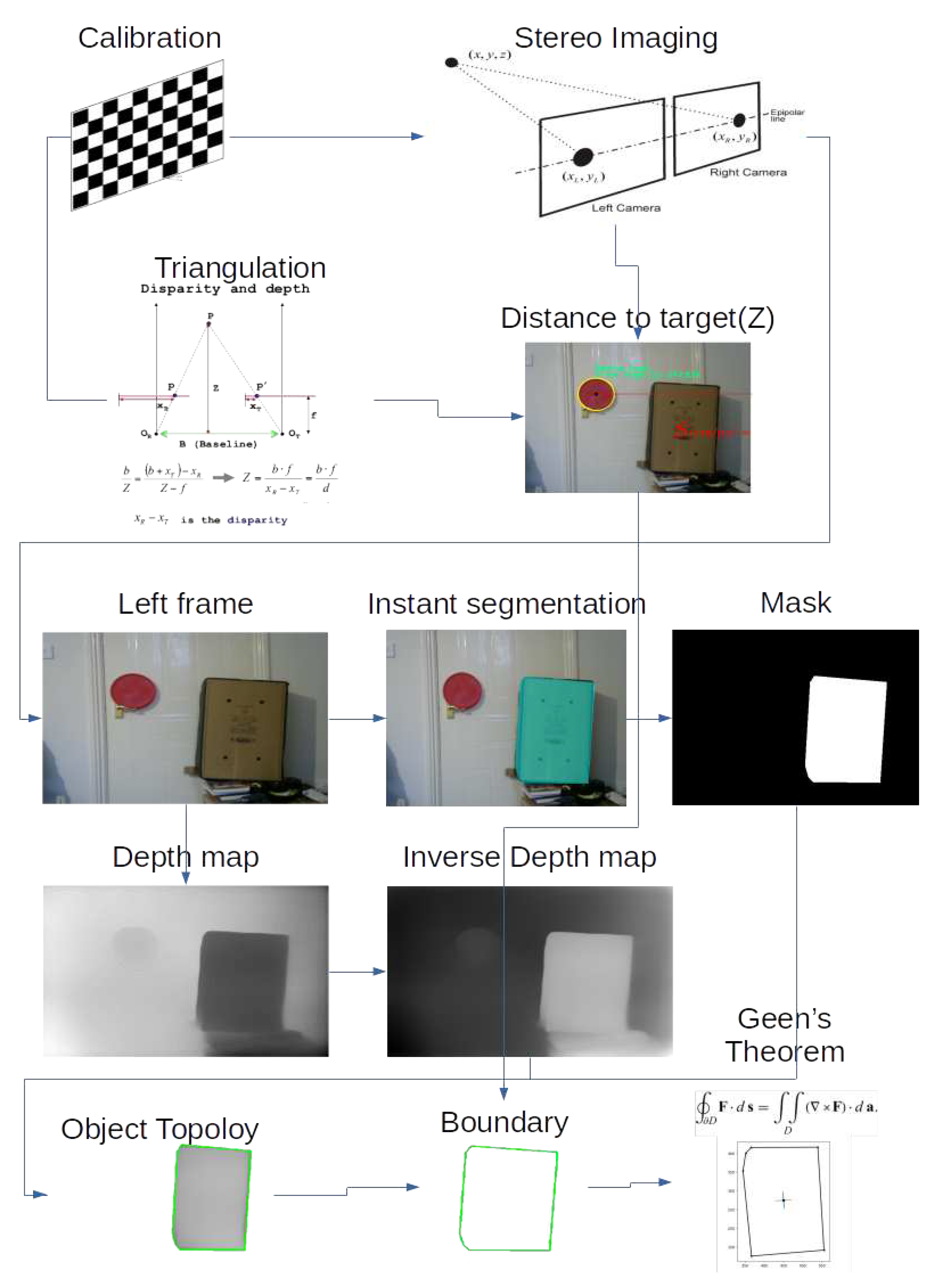
Figure 1. Pipeline.
Figure 1. Pipeline.
Preprints 80859 g001
Figure 2. Typical stereo-vision system.
Preprints 80859 g002
Figure 3. Illustration of image rectification. Epipolar lines e 1 , e 2 are projected on a common line (dashed red-green). The distance between principle points ( U l , V l ) and ( U R , V R ) along the common line is the baseline b. [68]
Preprints 80859 g003
Figure 4. Depth maps: Original image (left), Sparse (middle), Dense (right).
Preprints 80859 g004
Figure 5. S is the ratio of the absolute distance Z in the left image to the relative distance R from the depth map in the right image.
Preprints 80859 g005
Figure 6. Sample of images with concrete structures used to train our neural network model.
Preprints 80859 g006
Figure 7. Extraction of the object boundary.
Preprints 80859 g007
Figure 12. Experiment 2.
Preprints 80859 g012
Disclaimer/Publisher’s Note: The statements, opinions and data contained in all publications are solely those of the individual author(s) and contributor(s) and not of MDPI and/or the editor(s). MDPI and/or the editor(s) disclaim responsibility for any injury to people or property resulting from any ideas, methods, instructions or products referred to in the content.
Copyright: This open access article is published under a Creative Commons CC BY 4.0 license, which permit the free download, distribution, and reuse, provided that the author and preprint are cited in any reuse.
Prerpints.org logo

Preprints.org is a free preprint server supported by MDPI in Basel, Switzerland.

Subscribe

© 2024 MDPI (Basel, Switzerland) unless otherwise stated