Preprint

Article

Evolutionary Reinforcement Learning of Neural Network Controller for Acrobot Task – Part1: Evolution Strategy

Altmetrics

Downloads

103

Views

Comments

Hidehiko Okada^*

This version is not peer-reviewed

Submitted:

31 July 2023

Posted:

02 August 2023

You are already at the latest version

Alerts

Abstract

Evolutionary algorithms find applicability in the reinforcement learning of neural networks due to their independence from gradient-based methods. To achieve successful training of neural networks using evolutionary algorithms, careful considerations must be made to select appropriate algorithms due to the availability of various algorithmic variations. The author previously reported experimental evaluations on Evolution Strategy for reinforcement learning of neural networks, utilizing the pendulum control task. In this study, the Acrobot control task is adopted as another task. Experimental results demonstrate that ES successfully trained a Multi-Layer Perceptron to achieve a remarkable height of 99.85% concerning the maximum height. However, the trained MLP failed to maintain the chain end in an upright position throughout an episode. In this study, it was observed that employing 8 hidden units in the neural network yielded better results with statistical significance compared to using 4, 16, or 32 hidden units. Furthermore, the findings indicate that a larger population size in ES led to a more extensive exploration of potential solutions over a greater number of generations, which aligns with the previous study.

Keywords:

Subject: Computer Science and Mathematics - Artificial Intelligence and Machine Learning

1. INTRODUCTION

Neural networks can be effectively trained using gradient-based methods for supervised learning tasks, where labeled training data are readily available. In such cases, the errors between the neural network outputs and their corresponding target values can be observed, and these errors are utilized to perform backpropagation through the network. As a result, the node connection weights and biases are appropriately adjusted. However, when it comes to reinforcement learning tasks, where labeled training data are not provided, neural networks demand the utilization of gradient-free training algorithms. In these scenarios, traditional gradient-based methods are not applicable due to the absence of labeled data. Instead, alternative approaches that do not rely on gradients must be employed to train the neural networks effectively. Evolutionary algorithms [1,2,3,4,5] find applicability in the reinforcement learning of neural networks due to their independence from gradient-based methods. Another representative reinforcement learning technique is Q-learning [6,7,8]. Q-learning requires obtaining the reward, denoted as

r (t)

, associated with action

a (t)

taken at state

s (t)

to determine the subsequent action,

a (t + 1)

, at the given time step

t

. In contrast, evolutionary algorithms do not require

r (t)

at every step; instead, they evaluate the rewards after an episode is completed. Consequently, evolutionary algorithms alleviate the need for designing specific rewards for each state-action pair, providing a significant advantage in certain scenarios.

Evolution Strategy [9,10], Genetic Algorithm [11,12,13,14], and Differential Evolution [15,16,17] stand as representative evolutionary algorithms. To achieve successful training of neural networks using evolutionary algorithms, careful considerations must be made regarding: i) selecting appropriate algorithms due to the availability of various algorithmic variations, and ii) designing hyperparameters as they significantly impact performance. The author previously reported experimental evaluations on Evolution Strategy for reinforcement learning of neural networks, utilizing the pendulum control task [18]. In this study, the Acrobot control task is adopted as another task.

2. ACROBOT CONTROL TASK

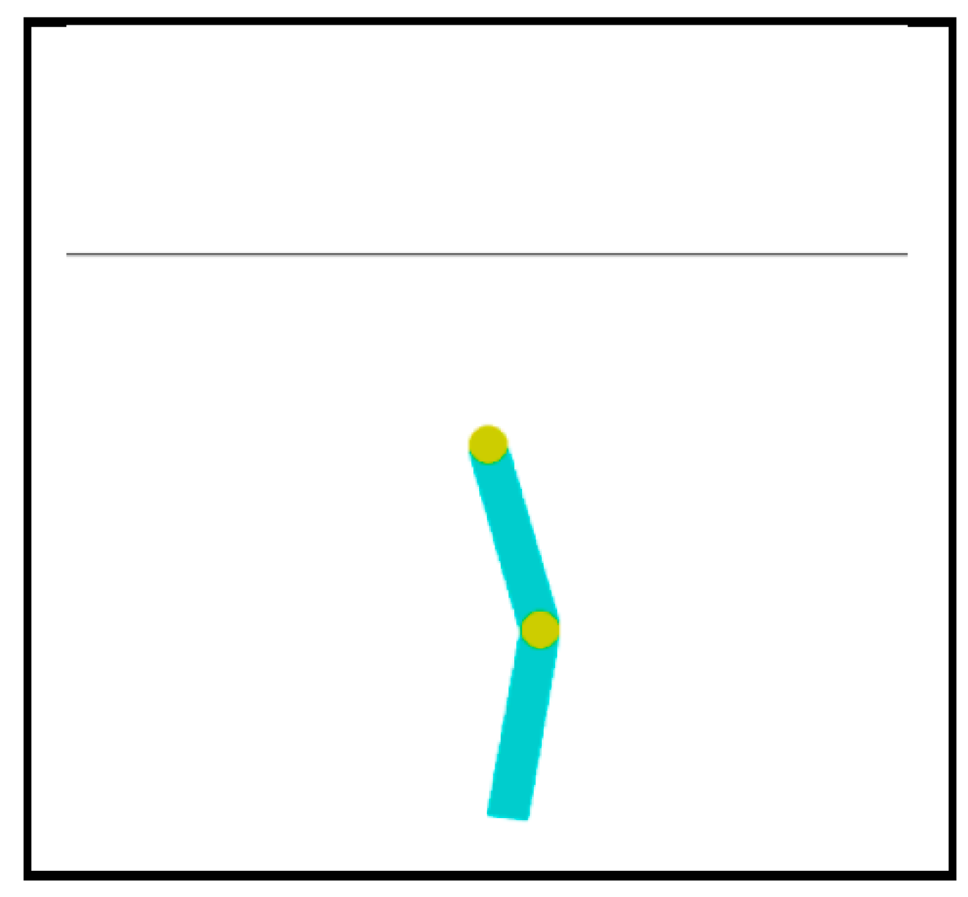
As a task that requires reinforcement learning to solve, this work employs Acrobot control task provided at OpenAI Gym. Figure 1 shows a screenshot of the system. The webpage for this system describes as follows1; The system consists of two links connected linearly to form a chain, with one end of the chain fixed. The joint between the two links is actuated. The goal is to apply torques on the actuated joint to swing the free end of the linear chain above a given height while starting from the initial state of hanging downwards.

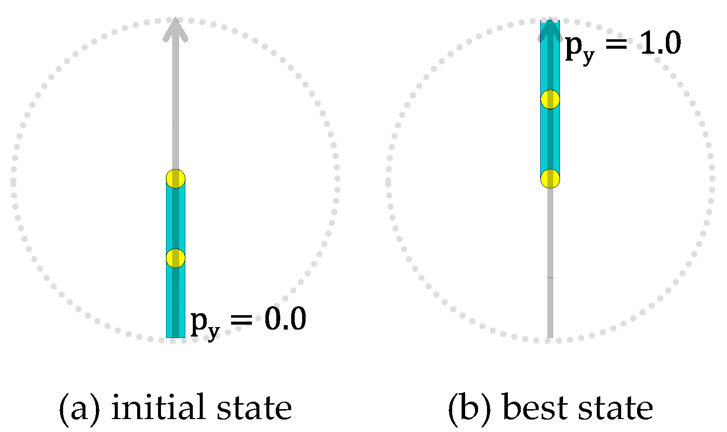
Let p_y denote the height of the free end of the linear chain, where the minimum (maximum) value of p_y is 0.0 (1.0) as shown in Figure 2. The goal of the task is originally to achieve p_y

\geq

0.5, and an episode is finished when the goal is achieved or the time step reaches to a preset limit. In this work, the goal is changed so that the free end of the linear chain is kept as high as possible (i.e., let the value of p_y as greater as possible) throughout an episode, where an episode consists of 200 time steps. Besides, the author changed the system so that (i) the control task starts with the state shown in Figure 2a where p_y=0.0, and (ii) the applicable torque to the actuated joint is continuous within [-1.0, 1.0] while the torque is originally discrete (either of -1, 0 or 1).

In each step, the controller observes the current state and then determines the action. An observation obtains cos(θ₁), sin(θ₁), cos(θ₂), sin(θ₂), and the angular velocity of θ₁ and θ₂, where θ₁ is the angle of the first joint and θ₂ is relative to the angle of the first link¹. The ranges are -1.0

\leq

cos(θ₁), sin(θ₁), cos(θ₂), sin(θ₂)

\leq

1.0,

- 4 π \leq

angular velocity of θ₁

\leq 4 π

, and

- 9 π \leq

angular velocity of θ₂

\leq 9 π

respectively.

In this work, the author defines the fitness of a neural network controller as shown in eq. (1).

F i t n e s s = \frac{1}{200} \sum_{t = 1}^{200} p_{y} (t),

(1)

In eq. (1), p_y(t) denotes the height p_y at each time step t. The fitness score is larger as p_y(t) is larger for more time steps. Thus, a controller fits better as it can keep the free end of the linear chain as higher as possible.

3. NEURAL NETWORKS

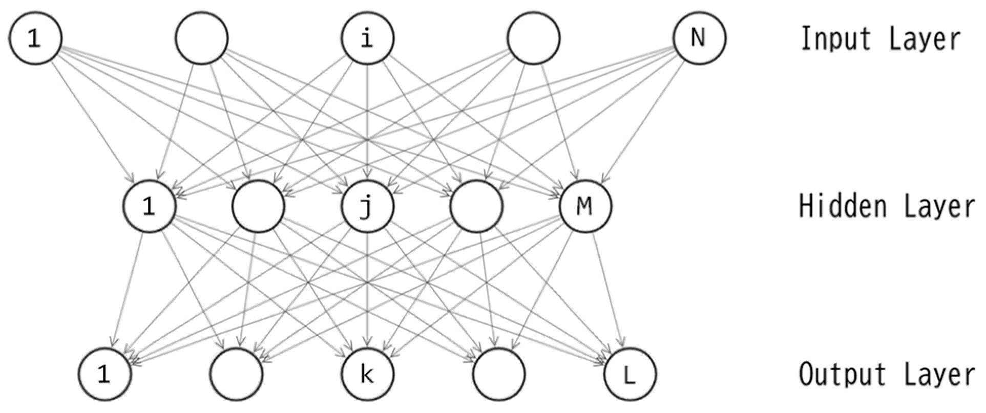
In this study, the author employs a three-layered feedforward neural network known as a multilayer perceptron (MLP [19,20]) as the controller. The topology of the MLP is illustrated in Figure 3, while eqs. (2)-(6) present the feedforward calculations.

Input layer:

{o u t}_{i}^{(1)} = x_{i}, i = 1,2, \dots, N

(2)

Hidden layer:

{i n}_{j}^{(2)} = θ_{j}^{(2)} + \sum_{i} w_{i, j}^{(2)} {o u t}_{i}^{(1)}, j = 1,2, \dots, M

(3)

{o u t}_{j}^{(2)} = h ({i n}_{j}^{(2)}), j = 1,2, \dots, M

(4)

Output layer:

{i n}_{k}^{(3)} = θ_{k}^{(3)} + \sum_{j} w_{j, k}^{(3)} {o u t}_{j}^{(2)}, k = 1,2, \dots, L

(5)

{o u t}_{k}^{(3)} = h ({i n}_{k}^{(3)}), k = 1,2, \dots, L

(6)

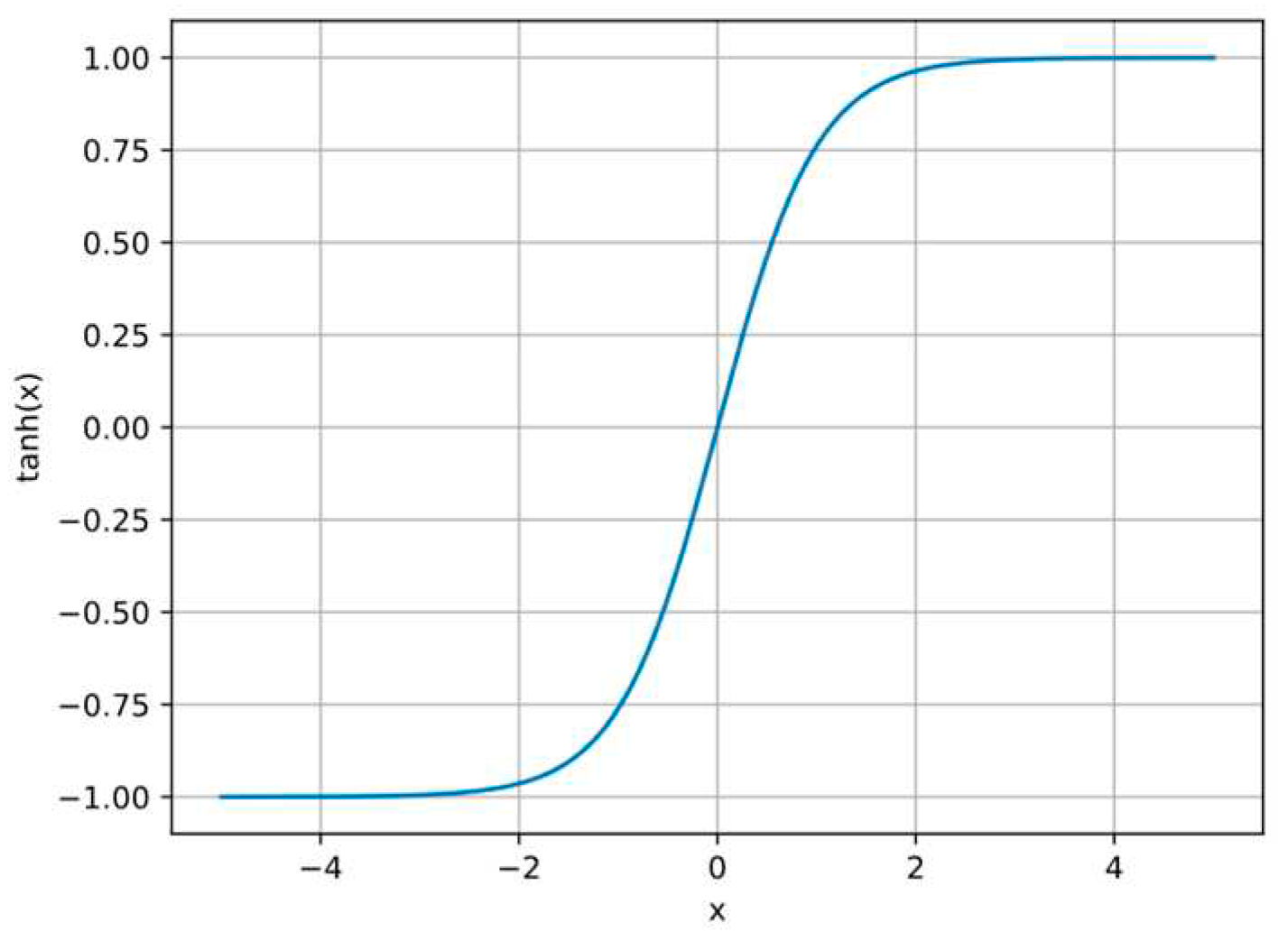
The activation function denoted as h() is the hyperbolic tangent function whose shape is illustrated in Figure 4. This activation function is widely used in neural networks due to its ability to produce a smooth non-linear output that ranges from -1.0 to 1.0.

h (x) = \frac{e^{x} - e^{- x}}{e^{x} + e^{- x}}

(7)

- 1.0 < h (x) < 1.0

(8)

In this study, the MLP serves as the policy function: action(t) = F(observation(t)). The input layer consists of six units, each corresponding to the values obtained by an observation. To ensure the input value falls within the range [-1.0, 1.0], the angular velocity of θ₁ (θ₂) is divided by

4 π

(

9 π

). The output layer comprises one unit, and its output value is directly applied as the torque to the joint.

4. TRAINING OF NEURAL NETWORKS BY EVOLUTION STRATEGY

A three-layered perceptron, as depicted in Figure 3, includes M+L unit biases and NM+ML connection weights, resulting in a total of M+L+NM+ML parameters. Let D represent the quantity M+L+NM+ML. For this study, the author sets N=6 and L=1, leading to D=8M+1. The training of this perceptron is essentially an optimization of the D-dimensional real vector. Let

x = (x_{1}, x_{2}, . . ., x_{D})

denote the D-dimensional vector, where each

x_{i}

corresponds to one of the D parameters in the perceptron. By applying the value of each element in

x

to its corresponding connection weight or unit bias, the feedforward calculation in eqs. (2)-(6) can be processed.

The process of training neural networks using evolutionary algorithms is known as neuroevolution [21,22]. Neuroevolution has found applications in various domains, including games [23,24,25,26]. For instance, Togelius et al. [26] utilized neuroevolution for simulated car racing. In this study, the D-dimensional vector

x

is optimized using Evolution Strategy [9,10]. ES treats

x

as a chromosome (a genotype vector) and applies evolutionary operators to manipulate it. The fitness of

x

is evaluated based on eq. (1).

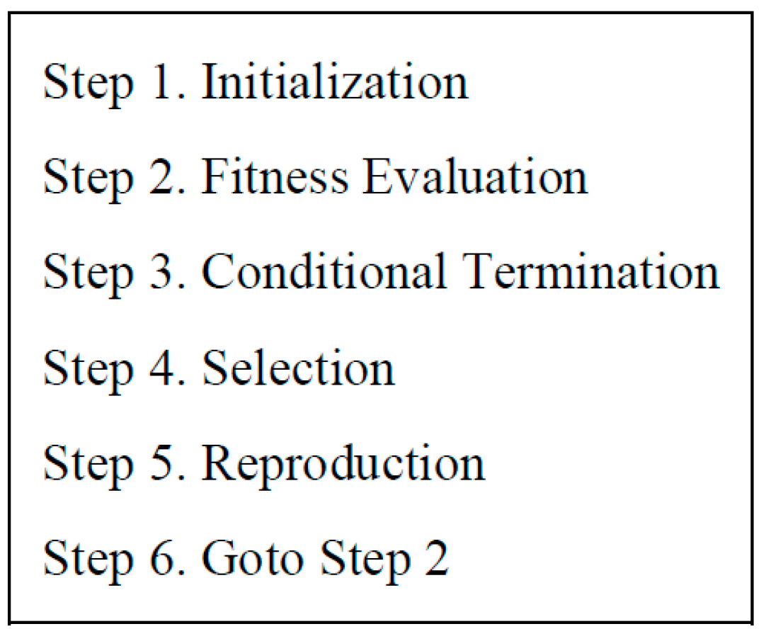
Figure 5 illustrates the ES process. Step 1 initializes vectors

y^{1}

y^{2}

, …,

y^{λ}

randomly within a predefined range, denoted as

{[m i n, m a x]}^{D}

, where

λ

represents the number of offsprings. A larger value of

λ

encourages more explorative search. In Step 2, the values in each vector

y^{c}

(c=1, 2, ...,

λ

) are fed into the MLP, which subsequently controls the Acrobot system for a single episode consisting of 200 time steps. The fitness of

y^{c}

is evaluated based on the outcome of the episode. In Step 3, the evolutionary training loop concludes upon meeting a preset condition. A straightforward example of such a condition is reaching the limit number of fitness evaluations. Proceeding to Step 4, from the

μ

vectors in the current parent population

z^{1}

z^{2}

, …,

z^{μ}

and the

λ

vectors in the current offspring population

y^{1}

y^{2}

, …,

y^{λ}

, only the vectors with the top

μ

fitness scores are selected to survive as parents in the next reproduction step, while the remaining vectors are discarded. Here,

μ

represents the number of parents. A smaller value of

μ

encourages more exploitative search. Note that the parent population is empty during the first occurrence of Step 4. Consequently, among the

λ

vectors in the current offspring population

y^{1}

y^{2}

, …,

y^{λ}

, only the vectors with the top

μ

fitness scores survive as parents. In Step 5, new

λ

offspring vectors are generated by applying the reproduction operator to the parent vectors

z^{1}

z^{2}

, …,

z^{μ}

selected in the previous Step 4. These newly produced offspring vectors form the updated offspring population

y^{1}

y^{2}

, …,

y^{λ}

. The process of reproduction is described in Figure 6.

y_{d}^{c} \leftarrow y_{d}^{c} + s * r a n d

(9)

i f y_{d}^{c} < m i n t h e n y_{d}^{c} \leftarrow m i n

(10)

i f \max < y_{d}^{c} t h e n y_{d}^{c} \leftarrow m a x

(11)

5. EXPERIMENT

The number of hidden units significantly impacts the MLP’s ability to model nonlinear functions. Utilizing evolutionary algorithms for optimizing a smaller MLP is advantageous, as it involves a reduced number of variables in the genotype vector

x

so that the search space is smaller. However, reducing the number of hidden units may hinder the MLP’s effectiveness in controlling the Acrobot system. On the other hand, a larger MLP will demonstrate better control performance, but optimizing it becomes more challenging due to the larger search space. Additionally, implementing a larger MLP demands more computational resources. Hence, finding a balance between these trade-offs is crucial to determine the optimal number of hidden units for the specific task. In this study, the author investigates four different configurations of hidden units: 4, 8, 16, and 32, to explore their impact on the system’s performance.

The ES hyperparameter values are determined through empirical analyses, as presented in Table 1. The number of generations is configured as either 500 or 100, corresponding to the population sizes (the number of offsprings

λ

) of 10 and 50, respectively. Consequently, the total number of fitness evaluations remains constant at 5,000, which is equivalent to the product of the number of generation and the population size.

Selecting an appropriate search domain is vital since the values in the genotype vector

x

serve as connection weights or unit biases in the neural network. The range should be chosen judiciously, neither excessively large nor small. For this experiment, the author sets

m i n

and

m a x

in eqs. (10) and (11) as -10.0 and 10.0 respectively.

An MLP with 4, 8, 16, or 32 hidden units underwent independent training 11 times. Table 2 presents the best, worst, average, and median fitness scores of the trained MLPs across the 11 trials. Each of the two hyperparameter configurations (a) and (b) in Table 1 was applied.

Upon comparing the scores in Table 2 between configurations (a) and (b), it is evident that the values obtained using configuration (b) are higher than those obtained using configuration (a). This result indicates that configuration (b) outperforms configuration (a). The Wilcoxon signed rank test confirmed that this difference is statistically significant (p<.01). Hence, in this study, increasing the population size, rather than the number of generations, allowed ES to discover superior solutions. In ES, augmenting the population size promotes global exploration during the initial stages, while increasing the number of generations enhances local exploitation during the later stages. Based on the findings of this experiment, it is apparent that early-stage global exploration is more critical for this learning task. This aligns with the author’s prior study [18], which employed a pendulum task instead of the Acrobot task.

Next, upon comparing the fitness scores obtained using configuration (b) among the four variations of M (the number of hidden units), it is observed that the scores with M=8 are better than those of M=4, 16 or M=32. The Wilcoxon rank sum test confirmed that the difference between M=8 and either of M=4, M=16 or M=32 is statistically significant (p<.01, p<.05 and p<.05 respectively). This observation suggests two conclusions: (i) 4 hidden units are not sufficient for this task, and (ii) 16 or more hidden units are excessive, resulting in an excessively large search space for ES with configuration (b).

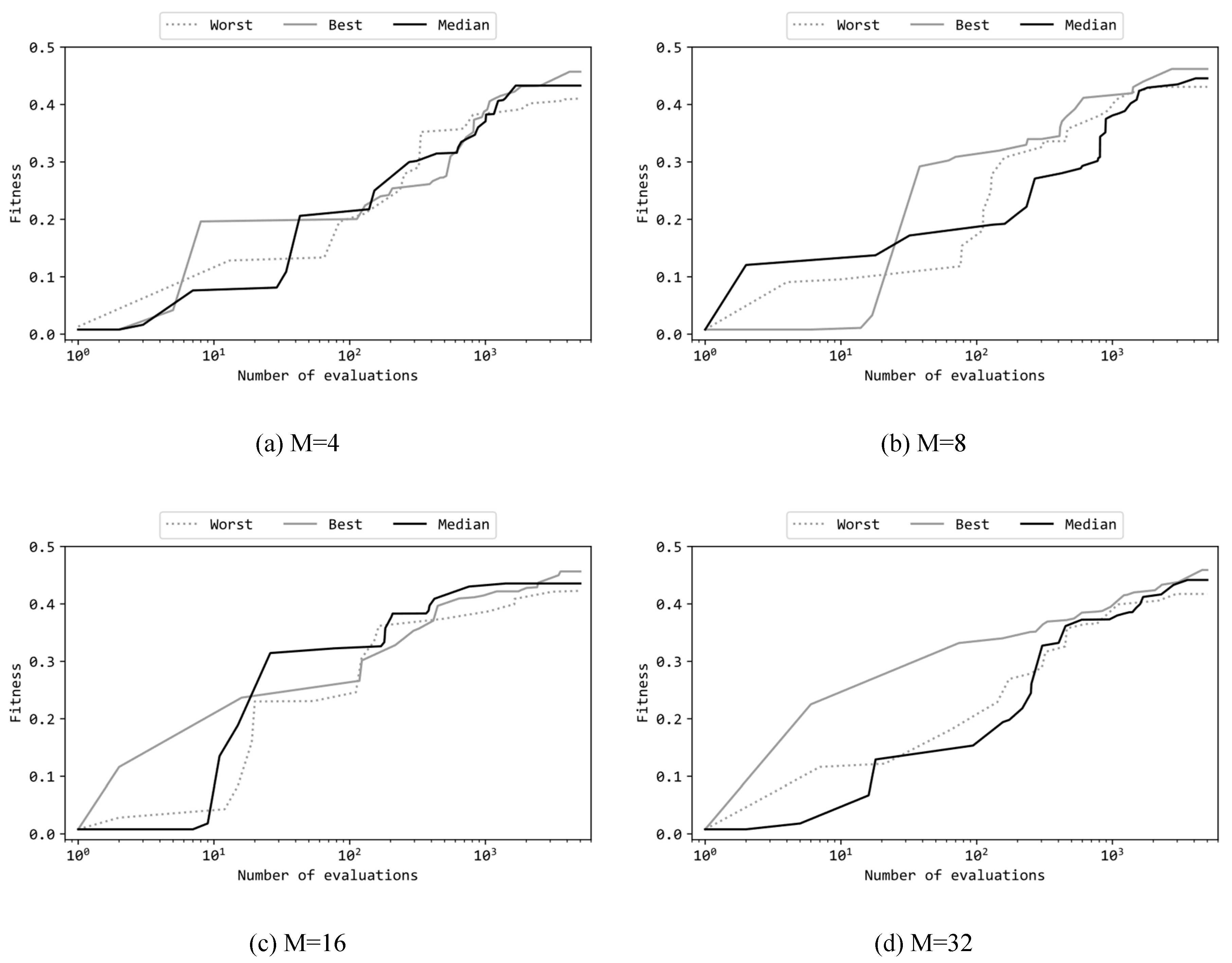
Figure 7 presents learning curves of the best, median, and worst runs among the 11 trials where the configuration is (b). Note that the horizontal axis of these graphs is in a logarithmic scale. The random solution for the first evaluation have fitness values almost exclusively at 0.0. The graphs in Figure 7 show increases in fitness from 0.1 to 0.2 by approximately the first 100 evaluations, which corresponds to 2% of the total 5,000 evaluations. Afterward, over the remaining 4,900 evaluations, the fitness gradually rises to around 0.4 to 0.45. For all the four M variations, even in the worst trials the final fitness scores are not significantly worse than the corresponding best trials. This indicates that ES could robustly optimize the MLP so that the variance was small within the 11 trials.

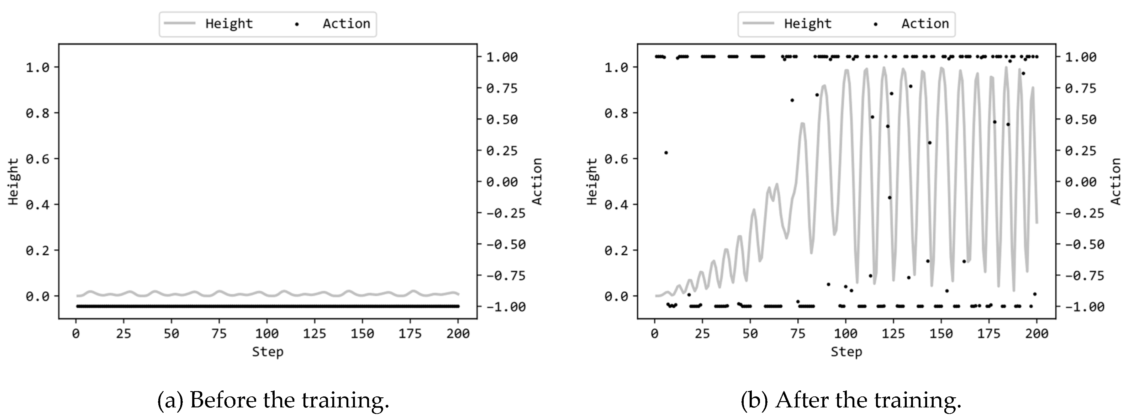
Figure 8a illustrates the actions by the MLP and the heights p_y(t) (see eq. (1)) in the 200 steps prior to training, while Figure 8b displays the corresponding actions and heights after training. In this scenario, the MLP employed 8 hidden units, and the configuration (b) was utilized. Figure 8a reveals that the MLP before training consistently provides a torque of -1.0 regardless of the system’s state, resulting in the chain end hardly rising from the bottom. On the other hand, as seen in Figure 8b, the MLP after training outputs alternating torques of -1.0 and 1.0, occasionally providing intermediate torque values as well. From the graph of p_y(t), it is evident that the chain gradually swings, causing the height of the end to rise, reaching 0.9850 at 100 steps. The best score of p_y(t) was 0.9985 at 183 steps, which is 99.85% of the maximum height. However, the MLP does not maintain the chain end in the upright position, and the value of p_y(t) oscillates between around 1.0 and 0.1. In this system, the torque is applied to the joint of the chain. Therefore, it is relatively easy to raise the height of the joint, but maintaining the chain’s free end at the upright position is difficult, as observed from the results. Supplementary videos are provided which demonstrate the motions of the chain2,3.

6. Conclusion

The author conducted an empirical application of Evolution Strategy to the reinforcement learning of a neural network controller for the Acrobot task. The experimental results demonstrated that ES successfully trained the multilayer perceptron to achieve a remarkable height of 99.85% concerning the maximum height. However, the trained MLP failed to maintain the chain end in an upright position throughout an episode.

In this study, it was observed that employing 8 hidden units in the neural network yielded better results with statistical significance compared to using 4, 16, or 32 hidden units. This suggests that selecting an appropriate number of hidden units is crucial, as an excessive number may not contribute to improved performance. Furthermore, the findings indicate that a larger population size in ES led to a more extensive exploration of potential solutions over a greater number of generations. This result aligns with the previous study by the author. However, to establish the generality of this observation, further investigations are necessary to verify if this holds true for evolutionary algorithms other than ES. Besides, the author intends to conduct additional evaluations to enhance evolutionary algorithms by applying them to diverse reinforcement learning tasks beyond the Acrobot task.

Acknowledgments

The author conducted this study under the Official Researcher Program of Kyoto Sangyo University.

References

Bäck, T., & Schwefel, H. P. (1993). An overview of evolutionary algorithms for parameter optimization. Evolutionary computation, 1(1), 1-23. [CrossRef]
Fogel, D. B. (1994). An introduction to simulated evolutionary optimization. IEEE transactions on neural networks, 5(1), 3-14. [CrossRef]
Bäck, T. (1996). Evolutionary algorithms in theory and practice: evolution strategies, evolutionary programming, genetic algorithms. Oxford university press.
Eiben, Á. E., Hinterding, R., & Michalewicz, Z. (1999). Parameter control in evolutionary algorithms. IEEE Transactions on evolutionary computation, 3(2), 124-141.
Eiben, A. E., & Smith, J. E. (2015). Introduction to evolutionary computing. Springer-Verlag Berlin Heidelberg.
Watkins, C. J. C. H. (1989). Learning from delayed rewards. PhD Thesis, Cambridge University.
Dayan, P., & Watkins, C. J. C. H. (1992). Q-learning. Machine learning, 8(3), 279-292.
Sutton, R. S., & Barto, A. G. (2018). Reinforcement learning: An introduction. MIT press.
Schwefel, H. P. (1984). Evolution strategies: A family of non-linear optimization techniques based on imitating some principles of organic evolution. Annals of Operations Research, 1(2), 165-167. [CrossRef]
Beyer, H. G., & Schwefel, H. P. (2002). Evolution strategies–a comprehensive introduction. Natural computing, 1, 3-52.
Goldberg, D.E., Holland, J.H. (1988). Genetic Algorithms and Machine Learning. Machine Learning 3, 95-99. [CrossRef]
Holland, J. H. (1992). Genetic algorithms. Scientific american, 267(1), 66-73.
Mitchell, M. (1998). An introduction to genetic algorithms. MIT press.
Sastry, K., Goldberg, D., & Kendall, G. (2005). Genetic algorithms. Search methodologies: Introductory tutorials in optimization and decision support techniques, 97-125.
Storn, R., & Price, K. (1997). Differential evolution–a simple and efficient heuristic for global optimization over continuous spaces. Journal of global optimization, 11, 341-359. [CrossRef]
Price, K., Storn, R. M., & Lampinen, J. A. (2006). Differential evolution: a practical approach to global optimization. Springer Science & Business Media.
Das, S., & Suganthan, P. N. (2010). Differential evolution: A survey of the state-of-the-art. IEEE transactions on evolutionary computation, 15(1), 4-31. [CrossRef]
Okada, H. (2022). Evolutionary reinforcement learning of neural network controller for pendulum task by evolution strategy, International Journal of Scientific Research in Computer Science and Engineering, 10(3), 13-18.
Rumelhart, D. E., Hinton, G. E., & Williams, R. J. (1986). Learning internal representations by error propagation. Parallel distributed processing: explorations in the microstructure of cognition, vol. 1: foundations. MIT Press, Cambridge, MA, USA, 318-362.
Collobert, R., & Bengio, S. (2004). Links between perceptrons, MLPs and SVMs. In Proceedings of the twenty-first international conference on Machine learning (ICML ‘04). Association for Computing Machinery, New York, NY, USA, 23. [CrossRef]
Yao, X., & Liu, Y. (1997). A new evolutionary system for evolving artificial neural networks. IEEE transactions on neural networks, 8(3), 694-713. [CrossRef]
Siebel, N. T., & Sommer, G. (2007). Evolutionary reinforcement learning of artificial neural networks. International Journal of Hybrid Intelligent Systems, 4(3), 171-183. [CrossRef]
Chellapilla, K., & Fogel, D. B. (1999). Evolving neural networks to play checkers without relying on expert knowledge. IEEE transactions on neural networks, 10(6), 1382-1391. [CrossRef]
Cardamone, L., Loiacono, D., & Lanzi, P. L. (2009). Evolving competitive car controllers for racing games with neuroevolution. In Proceedings of the 11th Annual conference on Genetic and evolutionary computation, 1179-1186.
Risi, S., & Togelius, J. (2015). Neuroevolution in games: State of the art and open challenges. IEEE Transactions on Computational Intelligence and AI in Games, 9(1), 25-41.
Togelius, J., & Lucas, S. M. (2005). Evolving controllers for simulated car racing. In 2005 IEEE Congress on Evolutionary Computation, 2, 1906-1913.

Figure 1. Acrobot system¹.

Figure 2. Initial and best states.

Figure 3. Topology of the MLP.

Figure 4. Hyperbolic tangent function.

Figure 5. Process of Evolution Strategy.

Figure 6. Process of reproduction in Evolution Strategy.

Figure 7. Learning curves of MLP with M hidden units.

Figure 8. MLP actions and the height p_y(t) in an episode.

Table 1. ES Hyperparameters.

Hyperparameters	(a)	(b)
Population size ( $λ$ )	10	50
Generations	500	100
Fitness evaluations	10 $\times$ 500=5,000	50 $\times$ 100=5,000
Number of parents ( $μ$ )	10 $\times$ 0.5=5	50 $\times$ 0.5=25
Step size ( $s$ )	1.0	1.0

Table 2. Fitness Scores among 11 Runs.

	M	Best	Worst	Average	Median
(a)	4	0.444	0.362	0.423	0.430
	8	0.455	0.386	0.431	0.434
	16	0.441	0.309	0.420	0.432
	32	0.437	0.349	0.413	0.416
(b)	4	0.457	0.410	0.430	0.433
	8	0.462	0.431	0.448	0.446
	16	0.457	0.423	0.437	0.436
	32	0.459	0.417	0.438	0.442

Notes

1	https://www.gymlibrary.dev/environments/classic_control/acrobot/
2	http://youtu.be/LfjE449vv3w
3	http://youtu.be/l24NLe1dIV4

Disclaimer/Publisher’s Note: The statements, opinions and data contained in all publications are solely those of the individual author(s) and contributor(s) and not of MDPI and/or the editor(s). MDPI and/or the editor(s) disclaim responsibility for any injury to people or property resulting from any ideas, methods, instructions or products referred to in the content.

© 2023 by the authors. Licensee MDPI, Basel, Switzerland. This article is an open access article distributed under the terms and conditions of the Creative Commons Attribution (CC BY) license (http://creativecommons.org/licenses/by/4.0/).

Copyright: This open access article is published under a Creative Commons CC BY 4.0 license, which permit the free download, distribution, and reuse, provided that the author and preprint are cited in any reuse.