Milling Mechanism and Chattering Stability of Nickel-Based Superalloy Inconel718

Nickel-based Superalloy Inconel 718 is widely used in the aerospace industry for its excellent high-temperature strength and thermal stability. However, milling Inconel 718 presents challenges due to significantly increased cutting force and vibration, which is a typical difficult-to-machine material. This paper focuses on the milling process of Inconel 718, establishing a milling force model to analyze the force trends under various processing parameters. Finite element analysis is employed to study the stress and temperature fields during milling. Dynamic equations for milling Inconel 718 are developed, and stability lobe diagrams are generated based on modal experiments. Milling experiments on Inconel 718 validate the milling force model and finite element analysis results. The fmincon optimization algorithm is utilized to identify the optimal machining parameters for Inconel 718. Through this research, valuable insights into enhancing the efficiency and quality of Inconel 718 machining are provided. This study contributes to a deeper understanding of Inconel 718 milling behavior, offering crucial guidance for more efficient machining processes.

Keywords:

Subject: Engineering - Mechanical Engineering

1. Introduction

Nickel-based Superalloy Inconel718 is widely used in the aerospace industry due to its extraordinary high-temperature strength, thermal stability, heat fatigue resistance, corrosion resistance, creep resistance, and oxidation resistance, especially in the field of manufacture of key components in the aerospace industry, such as turbine blades, combustion chamber components, and gas turbines[1,2,3,4]. Common processing methods for Inconel718 are mainly casting[5], forging[6], laser processing[7] and electrical discharge machining[8]. However, each of these machining methods suffers from flaws like low dimensional accuracy, inability to process complex geometry, high machining costs and containing heat-affected areas, slow machining speed, and poor surface quality respectively. Although utilizing the milling method can effectively avoid the above-mentioned problems, Inconel718 in the cutting process is prone to serious tool wear, high thermal stress, high cutting forces, vibration, and other phenomena[9]. In order to address these challenges and improve the machinability of Inconel718, the milling mechanisms and chattering stability of Inconel718 need to be investigated. Based on this, the optimized processing parameters could be determined by analyzing the influence of different processing parameters, such as spindle speed, feed per tooth, radial depth of cut, and axial depth of cut on cutting force, temperature, stress, and deformation, including machining quality during manufacturing.

Accurate modeling of milling force can help adjust cutting parameters to ensure high-quality machining results, therefore, it is especially necessary to establish an accurate milling force model. At present, the milling force models proposed by scholars mainly include empirical models, physical analytical models, and finite element models.

The empirical model of milling force is a model derived by fitting milling test data and is mainly used to predict the magnitude of milling force. Ding[10], Zhao[11], and Lei[12] used orthogonal tests to obtain the milling force coefficients and established an empirical model of milling force. Bergmann[13] developed a nonlinear empirical model of milling force and improved the prediction of stability limits achieved by parameterizing a milling force model for stability analysis. Zhao[14] established an empirical model of milling force for ultrasonic vibration milling of titanium alloy and explored the effects of different machining parameters on milling force. Liang[15] proposed an empirical model of cutting forces in micro-end-milling operations that takes into account the parameters of feed per tooth per tool radius, the true trochoidal nature of the tool edge path, and the chip thickness. Li[16] established an empirical model for the prediction of milling force and cutting temperature based on the multiple linear regression method. In fact, the empirical model of milling force relies on a large amount of experimental data and has obvious limitations, which cannot reveal the dynamic characteristics and mechanism of cutting, and can only be used to calculate the average milling force, rather than accurately predict the instantaneous cutting force during the milling process.

A physical analytical model of milling force is a model that describes the cutting forces generated during the milling process with the help of mathematical analytical methods. The physical analytical model of milling force is usually based on the basic theories of machining principles and material mechanics. Jiang[17] proposed that the projected area of the milling shear surface in three directions determines the milling force in three directions, and established an analytical model of milling force based on the shear surface. Madajewski[18] presented a computational method based on a combination of finite element analysis and classical analytical methods for predicting the cutting force components in face milling processes. Wang[19] discretized the end milling cutter along the circumferential direction and established an analytical cutting force model for the end milling cutter and simplified analytical indexes for predicting and estimating cutting force fluctuations. Kao[20] developed a mathematical model of the cutting forces of a ball-end milling cutter that includes tangential, radial, and axial cutting force components, and characterized the relationship between average cutting force and feed per groove as a linear function. Zhou[21], Kazuki[22], and Li[23] modeled the milling force of a ball-end milling cutter considering changes of microelement friction angle, shear angle, and shear stress constraints using microelement diagonal shear theory. Falta[24] and Dong[25] used an analytical modeling method for predicting the static milling force of a ball-end milling cutter by establishing a tool-workpiece engagement region. The removal mechanism of materials can be deeply analyzed through the physical analytical model; however, the physical analytical model is closely related to material constitutive parameters, which are difficult to obtain. Therefore, the physical analytical model is not convenient for practical application, and its modeling process is complex and cumbersome.

Finite element model of milling force is a mathematical model that predicts milling forces and contact forces during the cutting process by discretizing the material regions being milled into small finite element regions. Li[26] used ABAQUS software to analyze the effects produced by polycrystalline diamond tools for machining thin walls of SiCp/Al composite material. Jin[27] established an optimized finite element model based on pendulum motion, considered the performance parameters of the workpiece, and used ABAQUS software to study the rule of change of milling force during the milling process of aerospace thin-wall component. Hu[28] modeled the thermal-mechanical coupling property of ultrasonic torsional vibration-assisted micro-milling (UTVAM) using ABAQUS software. Pratap[29] used the Johnson-Cook constitutive equation to develop a finite element model for micro-channel micro-end milling of titanium alloys using ABAQUS that takes into account the strain, strain rate, and temperature effects on material properties. Li[30] imported the blade model created using UG NX into ANSYS software for simulation of milling force and calculated the elastic deformation of the blade using both MATLAB and ANSYS. The finite element model of milling force can simulate the real milling process, consider the contact and interaction between the tool and the workpiece, and is able to predict the mechanical properties and deformation behavior. However, the use of different finite element models will lead to different accuracy results. Therefore, it is recommended that a higher precision, more targeted finite element model should be chosen to accurately and intuitively simulate the milling process.

Chattering is an unstable state of motion in metal cutting processing, mainly caused by cutting force, cutting heat, and material deformation. Inconel718 is difficult-to-machine material, and its high hardness and heat resistance make it more susceptible to chattering during the milling process. At present, the theoretical analysis methods for milling stability mainly include frequency domain analysis and time domain analysis.

The frequency domain analysis is a method used to evaluate and solve the chattering problem in the milling process by converting the dynamic response of the milling system to the frequency domain. Frequency domain analysis method can be further divided into zero-order frequency domain method and multi-frequency method. Altintaş and Budak[31] proposed a zero-order frequency domain method of milling stability, in which the oriented dynamic milling force coefficient matrix is transformed into the frequency domain by Fourier transform to solve for the stability of the system without taking into account the cross-transfer function of the system. Based on that, the critical axial depth of cut without causing chattering is determined. Merdol[32] considered the higher-order expansion terms of the Fourier series of the oriented dynamic milling force coefficient matrix and gave a multi-frequency method that can be used in different radial depths of cut cases.

The time domain analysis is another method used to evaluate and solve the chattering problem in the milling process by observing and analyzing the time response. The time domain analysis method can be further divided into fully-discrete and semi-discrete methods. Ding[33,34] verified the accuracy of the method by single-degree-of-freedom and two-degree-of-freedom milling models and then proposed the second-order full-discrete method. Insperger[35,36,37] proposed a semi-discrete method to solve a system of time-delay differential equations containing a matrix of periodic coefficients. Subsequently, the method is improved so that it can not only solve the stability limit of a single-degree-of-freedom vibration system, but also a two-degree-of-freedom vibration system, and the first-order semi-discrete method with better convergence is proposed. Based on the semi-discrete method, Sun[38] established the stability lobe diagram of rotary ultrasonic milling of titanium alloy by defining the ultrasonic function angle, and the results showed that the rotary ultrasonic milling can suppress the machining vibration and improve the stability of milling of titanium alloy.

In this paper, the milling force model of a ball-end milling cutter is established by analytical method, additionally, both the experimental and finite element analysis is carried out. Since the material studied in this paper is Inconel718, which is prone to chattering and can easily lead to machining instability. Besides, the zero-order frequency domain method is computationally efficient and suitable for general processing situations, so this paper adopts the zero-order frequency domain method.

2. Modeling of Milling Forces

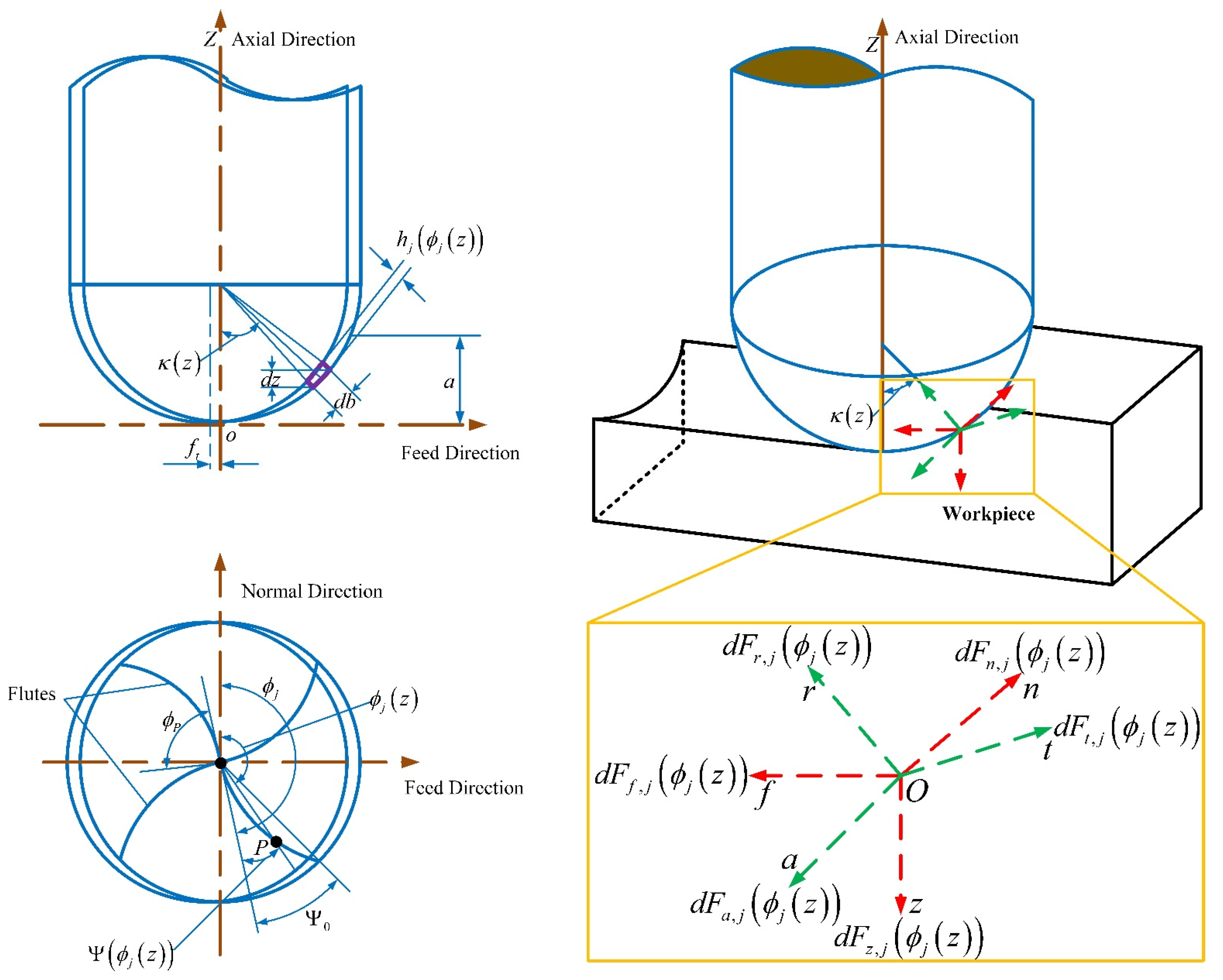
2.1 Modeling of Milling Forces of Ball-End Milling Cutter

The milling state of the helix cutting edge of the ball-end milling cutter varies with different cutting positions. Thus, it is essential to develop a geometric model of the ball-end milling cutter to investigate the milling force changes when the cutting edge interacts with the workpiece. The schematic of the proposed model is illustrated in Figure 1.

Figure 1 Milling force model of ball-end milling cutter.

According to the literature[20], neglecting the tip radius of the ball-end milling cutter results in the cutting force on any microelement of the cutting edge being described by equation (1).

{\begin{cases} d F_{t, j} (ϕ_{j} (z)) = K_{t e} d S (ϕ_{j} (z)) + K_{t c} h_{j} (ϕ_{j} (z)) d b \\ d F_{r, j} (ϕ_{j} (z)) = K_{r e} d S (ϕ_{j} (z)) + K_{r c} h_{j} (ϕ_{j} (z)) d b \\ d F_{a, j} (ϕ_{j} (z)) = K_{a e} d S (ϕ_{j} (z)) + K_{a c} h_{j} (ϕ_{j} (z)) d b \end{cases}

(1)

The instantaneous chip thickness at the immersion angle

h_{j} (ϕ_{j} (z))

can be expressed as:

h_{j} (ϕ_{j} (z)) = f_{t} \sin (ϕ_{j} (z)) \sin (κ (z))

(2)

The instantaneous edge length of the cutting segment

d S (ϕ_{j} (z))

can be expressed as:

d S = d z \cdot \sqrt{\frac{{(R_{0} - z)}^{2}}{R_{0}^{2} - {(R_{0} - z)}^{2}} + \frac{\tan^{2} β}{R_{0}^{2}} [R_{0}^{2} - {(R_{0} - z)}^{2}] + 1} = M \cdot d z

(3)

The instantaneous chip width

d b

can be expressed as:

d b = \frac{d z}{\sin (κ (z))} = \frac{R_{0}}{\sqrt{R_{0}^{2} - {(R_{0} - z)}^{2}}} d z

(4)

By transforming the cutting force microelement from a coordinate system

O - t r a

O - f n z

and integrating it, the cutting force of the milling cutter along feed, normal and axial directions can be obtained as:

[\begin{matrix} F_{f} (ϕ) \\ F_{n} (ϕ) \\ F_{z} (ϕ) \end{matrix}] = [\begin{matrix} \sum_{j = 1}^{N} F_{f, j} (ϕ_{j}) \\ \sum_{j = 1}^{N} F_{n, j} (ϕ_{j}) \\ \sum_{j = 1}^{N} F_{z, j} (ϕ_{j}) \end{matrix}]

(5)

Subsequently, the average milling force per rotation of the ball-end milling cutter can be calculated using the equation (6):

{\begin{cases} \bar{F_{f}} = \frac{N_{f}}{2 π} \int_{0}^{2 π} (\int_{z_{1} (ϕ_{j})}^{z_{2} (ϕ_{j})} d F_{f} (ϕ_{j} (z))) d ϕ \\ \bar{F_{n}} = \frac{N_{f}}{2 π} \int_{0}^{2 π} (\int_{z_{1} (ϕ_{j})}^{z_{2} (ϕ_{j})} d F_{n} (ϕ_{j} (z))) d ϕ \\ \bar{F_{z}} = \frac{N_{f}}{2 π} \int_{0}^{2 π} (\int_{z_{1} (ϕ_{j})}^{z_{2} (ϕ_{j})} d F_{z} (ϕ_{j} (z))) d ϕ \end{cases}

(6)

Equation (7) is finally obtained by simplifying the equation of the microelement of milling force and substituting it into (6):

{\begin{cases} {\bar{F}}_{f} = (C_{1} K_{t c} + C_{3} K_{r c} + C_{5} K_{a c}) f_{t} + C_{2} K_{t e} + C_{4} K_{r e} + C_{6} K_{a e} \\ {\bar{F}}_{n} = (C_{7} K_{t c} + C_{9} K_{r c} + C_{11} K_{a c}) f_{t} + C_{8} K_{t e} + C_{10} K_{r e} + C_{12} K_{a e} \\ {\bar{F}}_{z} = (C_{13} K_{r c} + C_{15} K_{a c}) f_{t} + C_{14} K_{r e} + C_{16} K_{a e} \end{cases}

(7)

The parameters

C_{1} - C_{16}

in equation (7) have been given by reference[20].

2.2 Recognition Experiment of Milling Force Coefficients

In order to be able to accurately find out the milling force generated during milling processing, it is necessary to determine the milling force coefficients

K_{t e}

K_{r e}

K_{a e}

K_{t c}

K_{r c}

K_{a c}

in equation (7), therefore, recognition experiments of milling force coefficient are required.

For this experiment, the Sandvik 1B240-0800-XA 1630 carbide ball-end milling cutter is chosen, the diameter of the cutter is 8mm, the overall length of the cutter is 100mm, the length of the cutting section is 25mm, the depth of cut is set to 0.5mm and the rotating speed of spindle is set to 1000rpm. In order to facilitate the calculation of milling force coefficients, slot milling is used as the milling method, and the selected machining parameters and the measured average milling force data are recorded in Table 1.

Based on data in Table 1, the scatter plot is plotted and the milling force coefficient is obtained by calculating the slope and intercept using the coefficient recognition equation of milling force (8).

{\begin{cases} K_{a c} = \frac{{\bar{F}}_{z c} (C_{3} C_{7} C_{15} - C_{1} C_{9} C_{15}) - C_{7} C_{13} C_{15} {\bar{F}}_{f c} + C_{1} C_{13} C_{15} {\bar{F}}_{n c}}{C_{3} C_{7} C^{2}_{15} - C_{5} C_{7} C_{13} C_{15} - C_{1} C_{9} C^{2}_{15} + C_{1} C_{11} C_{13} C_{15}} \\ K_{a e} = \frac{{\bar{F}}_{z e} (C_{4} C_{8} C_{16} - C_{2} C_{10} C_{16}) - C_{14} C_{8} C_{16} {\bar{F}}_{f e} + C_{2} C_{14} C_{16} {\bar{F}}_{n e}}{C_{4} C_{8} C^{2}_{16} - C_{6} C_{8} C_{14} C_{16} - C_{2} C_{10} C^{2}_{16} + C_{2} C_{12} C_{14} C_{16}} \\ K_{r c} = \frac{C_{7} C_{15} {\bar{F}}_{f c} - C_{1} C_{15} {\bar{F}}_{n c} + (C_{1} C_{11} - C_{5} C_{7}) {\bar{F}}_{z c}}{C_{3} C_{7} C_{15} - C_{5} C_{7} C_{13} - C_{1} C_{9} C_{15} + C_{1} C_{11} C_{13}} \\ K_{r e} = \frac{C_{8} C_{16} {\bar{F}}_{f e} - C_{2} C_{16} {\bar{F}}_{n e} + (C_{2} C_{12} - C_{8} C_{6}) {\bar{F}}_{z e}}{C_{4} C_{8} C_{16} - C_{6} C_{8} C_{14} - C_{2} C_{10} C_{16} + C_{2} C_{12} C_{14}} \\ K_{t c} = \frac{{\bar{F}}_{f c} - C_{3} K_{r c} - C_{5} K_{z c}}{C_{1}} \\ K_{t e} = \frac{{\bar{F}}_{f e} - C_{4} K_{r e} - C_{6} K_{z e}}{C_{2}} \end{cases}

(8)

Afterwards, a linear regression equation is formulated, taking the feed per tooth as the independent variable and the measured average milling force as the dependent variable. Figure 2 illustrates the milling force variation with changes in the feed per tooth along each axis, and Table 2 presents the coefficients of the milling force.

Figure 2 The relationship between average milling force and feed per tooth.

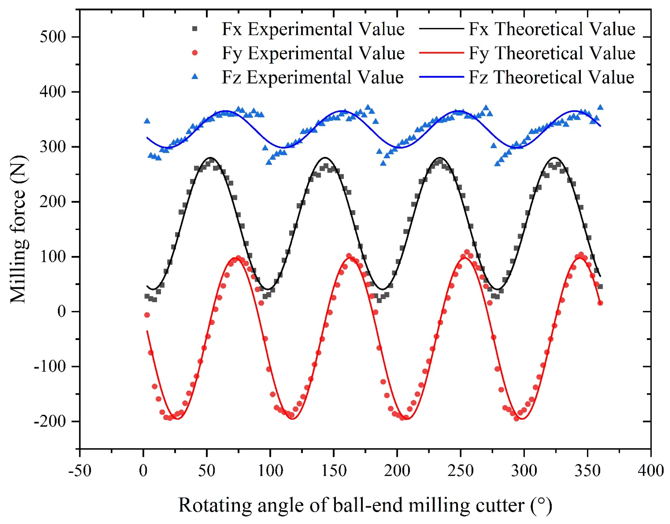
2.3 Validation of Milling Force Model for Ball-End Milling Cutter and Results Analysis

Based on the above-proposed milling force model of the ball-end milling cutter, the Matlab program, which is illustrated in the Appendix, is written to calculate the theoretical milling force. The results of the theoretical analysis are compared with the experimentally measured results to verify the correctness of the proposed milling force model. The same manufacturing parameters are set for both theoretical and experimental analysis, namely, the spindle speed is 1000rpm, the axial depth of cut is 0.4mm and the feed per tooth is 0.04mm/z. The results of the comparative analysis of the theoretical and experimental values of milling forces of the X, Y, and Z-axis are shown in Figure 3, observing the milling force values in each axis, it is evident that both the theoretical and experimental results exhibit a similar change trend, validating the accuracy of the proposed theoretical model for calculating the ball-end milling cutter's milling force. Although a slight degree of error is present in the figures, they remain within an acceptable range.

Figure 3 Experimental and theoretical comparison of milling forces.

The feed per tooth plays a pivotal role in determining both the magnitude of the milling force and the quality of the machined surface. Consequently, to investigate the influence of the feed per tooth on the milling forces, the different feed rate per tooth is set separately as

f_{z}

=0.1mm/z, 0.2mm/z, 0.3mm/z, 0.4mm/z, while keeping the radial depth of cut and axial depth of cut unchanged, namely

a_{e}

=3mm,

a_{p}

=0.5mm. In addition to feed per tooth, the tool helix angle is another important parameter that affects the milling process. Change in helix angle in ball-end milling cutter affects the cutting angle and feed angle, which in turn affects the contact between tool and workpiece. The tool helix angle is set separately as

β = 15 °

β = 25 °

β = 35 °

β = 45 °

in the case of ensuring other parameters remain unchanged. The results of above studies are shown in Figure 4 - Figure 6. When the feed per tooth of the ball-end milling cutter increases, there is a corresponding upward trend observed in the milling force for each axis. Similarly, an increase in the helix angle of the ball-end milling cutter results in a proportional rise in the cutting force. This can be attributed to the expansion of the contact area between the tool and the workpiece, leading to an overall mounting trend in cutting force along all axes. Due to the significant impact of the ball-end milling cutter's helix angle on the generated milling force in each axis, careful consideration and selection of the appropriate tool helix angle are imperative to meet specific machining requirements

3. Finite Element Analysis of Milling of Inconel718

In this study, firstly, a finite element model is established, as shown in Figure 7, including the workpiece and the tool. In the following, the temperature, stress and milling force in the milling process are calculated. Finally, the influence of different machining parameters on the machining condition of Inconel718 is evaluated through simulation results.

3.1. The Constitutive Model of Inconel718

The constitutive model is a critical prerequisite of accuracy and reliability of finite element analysis. The behavior of materials and results of engineering problem can be better provided by a right chosen constitutive model[39]. The constitutive models applicable to metal cutting are mainly Power Law and Johnson-Cook model[40]. The Power Law constitutive model is usually applicable to analysis of deformation behavior of materials at high temperatures and high strain rates, while the Johnson-Cook constitutive model is more suitable for analysis of deformation behavior of materials at low to medium temperatures and low to medium strain rates. Therefore, the deformation behavior of Inconel718 at high temperatures and high strain rates can be described using the Power Law constitutive model. The mathematical equation of Power Law model could be expressed as:

σ (ε^{p}, \dot{ε}, T) = g (ε^{p}) Γ (\dot{ε}) Θ (T)

(9)

In equation (9), the strain enhancement function

g (ε^{p})

could be further expressed as:

{\begin{cases} g (ε^{p}) = σ_{0} {(1 + \frac{ε^{p}}{ε_{0}^{p}})}^{1 / n} ε^{p} < ε_{c u t}^{p} \\ g (ε^{p}) = σ_{0} {(1 + \frac{ε_{c u t}^{p}}{ε_{0}^{p}})}^{1 / n} ε^{p} \geq ε_{c u t}^{p} \end{cases}

(10)

The strain enhancement parameters of Inconel718 are shown in Table 3.

In equation (9), the thermal softening function

Θ (T)

could be expressed as:

{\begin{cases} Θ (T) = c_{0} + c_{1} T + c_{2} T^{2} + c_{3} T^{3} + c_{4} T^{4} + c_{5} T^{6} T < T_{cut} \\ Θ (T) = Θ (T_{cut}) (1 - \frac{T - T_{cut}}{T_{melt} - T_{cut}}) T \geq T_{cut} \end{cases}

(11)

The thermal softening parameters of Inconel718 are shown in Table 4.

In equation (9), the strain rate effect function

Γ (\dot{ε})

could be expressed as:

{\begin{cases} Γ (\dot{ε}) = {(1 + \frac{\dot{ε}}{{\dot{ε}}_{0}})}^{\frac{1}{m_{1}}} \dot{ε} \leq {\dot{ε}}_{t} \\ Γ (\dot{ε}) = {(1 + \frac{\dot{ε}}{{\dot{ε}}_{0}})}^{\frac{1}{m_{2}}} {(1 + \frac{{\dot{ε}}_{t}}{{\dot{ε}}_{0}})}^{(\frac{1}{m_{1}} - \frac{1}{m_{2}})} \dot{ε} > {\dot{ε}}_{t} \end{cases}

(12)

The strain rate parameters of Inconel718 are shown in Table 5.

The damage model for Inconel718 can be determined by the following equation:

D = \sum_{i} \frac{Δ ε_{i}^{p}}{ε_{f_{i}}^{p}}

(13)

In equation (13), the parameter

Δ ε_{i}^{p}

could be expressed as:

ε_{f_{0}}^{p} = d_{0} + d_{1} T + d_{2} T^{2} + d_{3} T^{3} + d_{4} T^{4} + d_{5} T^{6}

(14)

In equation (14), the parameters

d_{0} \sim d_{5}

are the strain value deduced by tensile test.

3.2 The Result of Finite Element Analysis

In order to study the effect of different processing parameters such as spindle speed, feed per tooth, radial and axial depth of cut on the temperature, stress and cutting force generated during the milling process of Inconel718, parameters as shown in Table 6 are taken for finite element analysis.

3.2.1 Temperature Field Analysis of Milling Process

Inconel718 belongs to the difficult-to-machine materials, which has low thermal conductivity. The phenomenon of thermal mechanical coupling could occur during machining process, which results in residual stress and reduces the surface quality. Therefore, in order to effectively control tool wear and improve the surface integrity of the workpiece, the milling temperatures must be systematically studied and analyzed.

The fitted curves of the maximum temperature at different spindle speeds, feed per tooth, radial and axial depth of cut are plotted, according to the results of finite element analysis, these curves are shown in Figure 8 (a) – (d).

From Figure 8, it can be seen that the temperature increases as the spindle speed increases, this is mainly due to the fact that the friction phenomenon between the front (or back) of tool and workpiece becomes more intense as the spindle speed increases. Moreover, with the increase of radial depth of cut, axial depth of cut and feed per tooth, the temperature also increases, because rising of all these parameters makes the tool cut more material per unit of time, so the heat continues to accumulate.

3.2.2 Stress Field Analysis of Milling Process

Due to the high hardness and strength properties of Inconel 718, the milling process of this material is susceptible to stress concentration and crack formation. Stress field simulation enables the visualization of stress distribution on both the tool and workpiece surfaces during machining, facilitating a deeper understanding of the physical phenomena involved. Consequently, the impact of various machining parameters on stress can be predicted to mitigate stress concentration and prevent crack formation.

To investigate the impact of processing parameters on stresses during machining, the stress values in the top 10% of elements with the highest stresses on the tool are averaged and plotted as a function of time. Fitted curves representing stress variations at different spindle speeds, feed per tooth, radial and axial depths of cut are presented in Figure 9 (a) – (d).

From Figure 9, it is evident that an increase in spindle speed does not significantly affect the stress, as the material volume cut by the tool remains unchanged despite the enlargement of the spindle speed. Conversely, with the increment of feed per tooth, radial depth of cut, and axial depth of cut, there is a simultaneous rise in stress. This observation can be attributed to the larger volume of material being removed due to changes in these parameters.

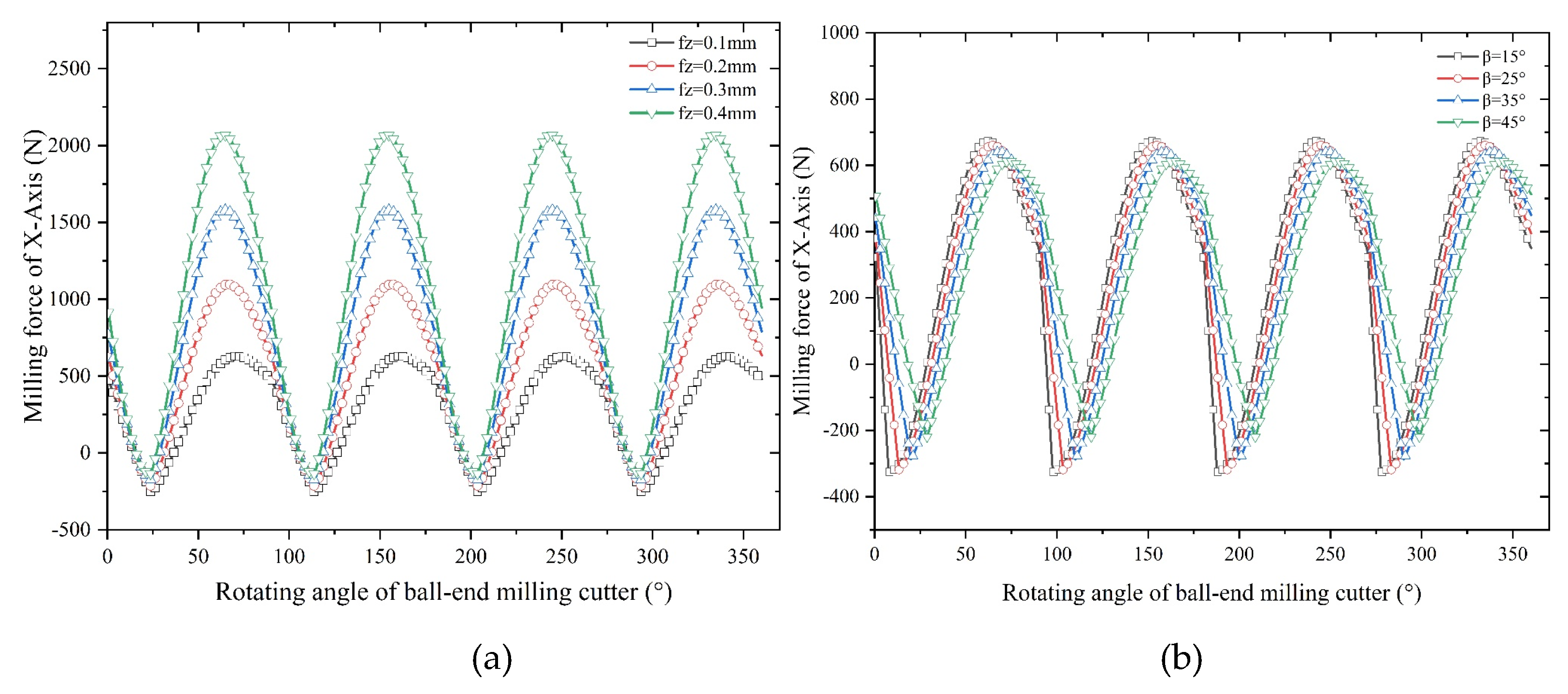
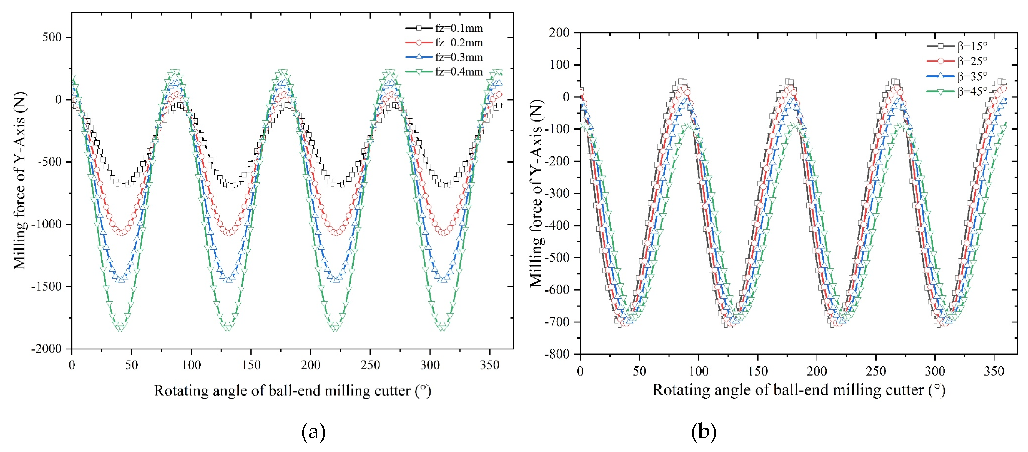
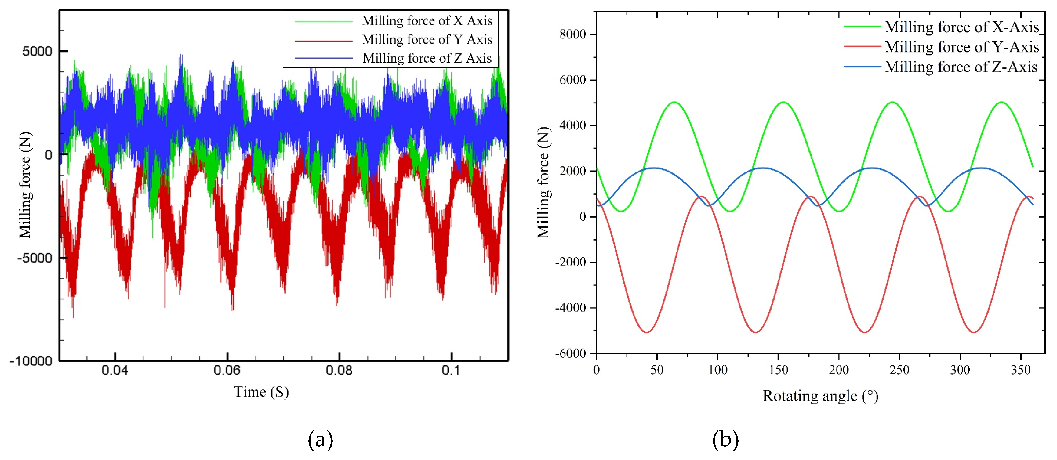
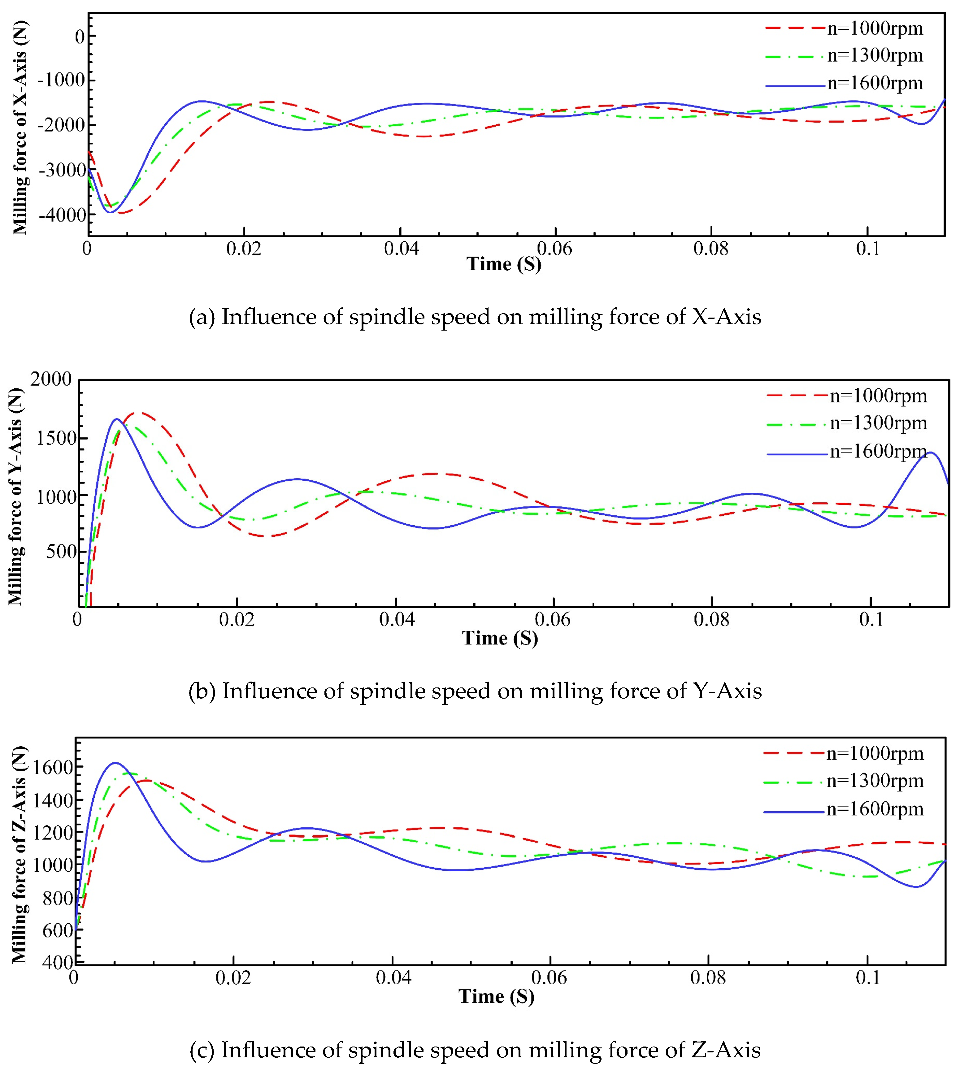
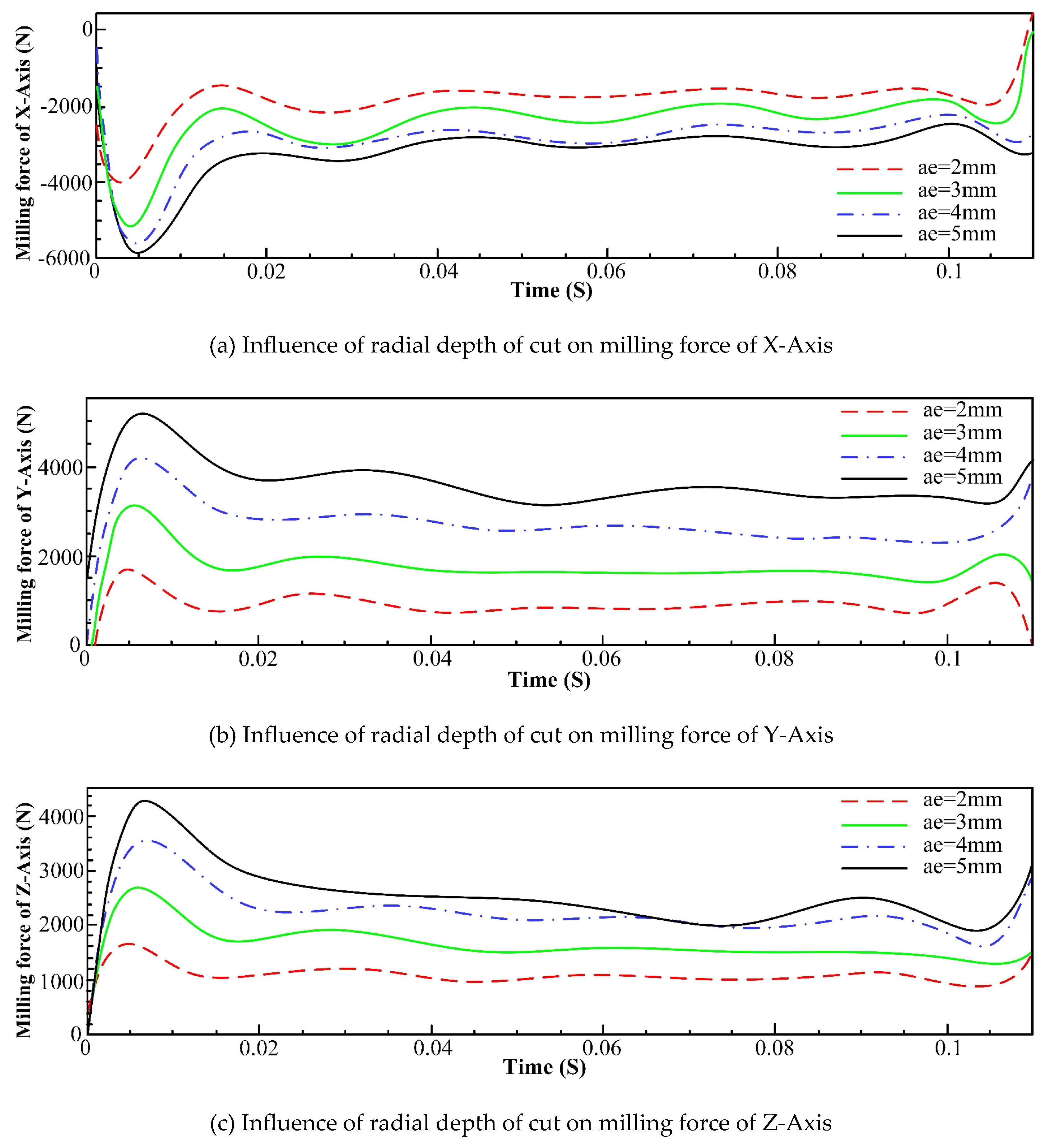
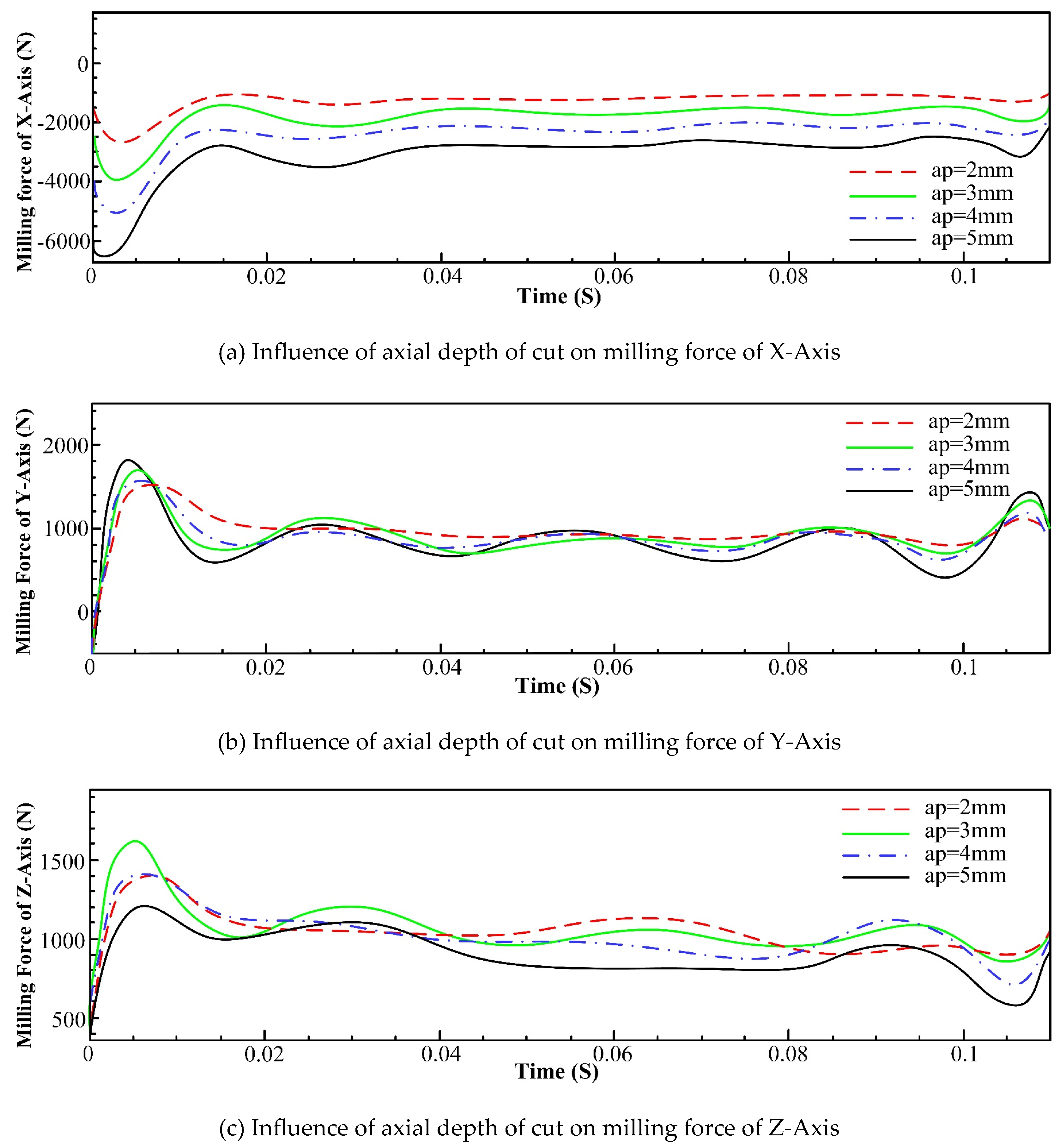
3.2.3 Force Analysis of Milling Process

Given that the magnitude of the milling force directly influences the wear and fracture condition of the tool, a comprehensive analysis of the milling force generated during the Inconel 718 milling process becomes crucial.

The milling forces measured through milling experiment are presented in Figure 10 (a), and the milling forces calculated by using the theoretical milling force model are presented in Figure 10 (b). The milling forces of each axis obtained from the theoretical model align closely with the experimental results, validating the accuracy and correctness of the proposed model.

In order to better study the influence trend of different machining parameters on milling force, spindle speed is set to 1000rpm, 1300rpm and 1600rpm respectively, other parameters are kept unchanged, the milling force data of each axis are shown in Figure 11.

Figure 11 illustrates that the effect of different spindle speeds on the magnitude of the milling force for each axis is not significant. This can be attributed to the nearly constant volume of material being removed, regardless of the spindle speed variation.

The feed per tooth is varied at values of 0.2 mm, 0.3 mm, 0.4 mm, and 0.5 mm, while keeping the remaining parameters unchanged. The corresponding milling force data for each axis is presented in Figure 12.

Figure 12 demonstrates a clear and consistent increasing trend in milling forces for each axis with the rise in feed per tooth. This observation can be attributed to the larger volume of workpiece material being removed by the cutter as the feed per tooth increases.

The radial depth of cut is varied at values of 2 mm, 3 mm, 4 mm, and 5 mm, while keeping the remaining parameters unchanged. The corresponding milling force data for each axis is presented in Figure 13.

Figure 13 reveals that the milling forces in the X-Axis, Y-Axis, and Z-Axis exhibit a notable increase with the rise in radial depth of cut. This observation can be attributed to the corresponding increase in the material removal rate, which occurs as the radial depth of cut is enlarged.

Similarly, the value of axial depth of cut is set to 2mm, 3mm, 4mm and 5mm respectively, and the rest of parameters are kept unchanged, the milling force data of each axis are shown in Figure 14.

4. Analysis of Milling Stability

Inconel718 belongs to difficult-to-machine materials, and is susceptible to the phenomenon of chattering during milling process. Chattering in the milling process will lead to a positive feedback effect between the cutting force and vibration, which will result in degradation of milling quality, cutting edge wear, tool fracture and other problems. Through the stability analysis of chattering, the stability condition of the milling process can be predicted, and whether chattering will occur during the milling process could also be determined. Therefore, it is necessary to carry out chattering stability analysis of Inconel718, so as to improve the milling efficiency and machining quality as well as reduce the production cost.

As shown in Figure 15, the machine-tool system is simplified as a vibration system with two degrees of freedom, where the vibrations in the X and Y directions can be described by the kinetic differential equations:

{\begin{cases} m_{x} \ddot{x} + c_{x} \dot{x} + k_{x} x = \sum_{j = 1}^{N} F_{x j} = F_{x} (t) \\ m_{y} \ddot{y} + c_{y} \dot{y} + k_{y} y = \sum_{j = 1}^{N} F_{y j} = F_{y} (t) \end{cases}

(15)

In the milling process, as shown in Figure 16, the current cutting process will be affected by the previous cutting process, since the previous machining process leaves vibration on the machined surface, and when the tool cut the surface again can lead to changes in the cutting thickness. Such changes in the cutting thickness can cause fluctuations in cutting force, leading to further vibration in the system. The total cutting thickness generated by the superposition of the static cutting thickness and the dynamic cutting thickness caused by tool vibration can be expressed as:

h (ϕ_{j}) = [f_{t} \sin ϕ_{j} + (v_{j, 0} - v_{j})] g (ϕ_{j})

(16)

In equation (16), the parameter

g (ϕ_{j})

is a unit step function, which is expressed below:

g (ϕ_{j}) = {\begin{cases} 1, (ϕ_{s t} < ϕ_{j} < ϕ_{e x}) \\ 0, (ϕ_{j} < ϕ_{s t} ， ϕ_{j} > ϕ_{e x}) \end{cases}

(17)

Therefore, the total cutting force on the cutter can be expressed as:

{\begin{matrix} F_{x} \\ F_{y} \end{matrix}} = \frac{1}{2} a_{p} K_{t c} [\begin{matrix} α_{x x} & α_{x y} \\ α_{y x} & α_{y y} \end{matrix}] {\begin{matrix} Δ x \\ Δ y \end{matrix}}

(18)

In equation (18) the parameters

α_{x x}

α_{x y}

α_{y x}

and

α_{y y}

are average directional force coefficient:

{\begin{cases} α_{x x} = \sum_{j = 0}^{N - 1} - g_{j} [\sin 2 ϕ_{j} + K_{r} (1 - \cos 2 ϕ_{j})] \\ α_{x y} = \sum_{j = 0}^{N - 1} - g_{j} [(1 + \cos 2 ϕ_{j}) + K_{r} \sin 2 ϕ_{j}] \\ α_{y x} = \sum_{j = 0}^{N - 1} g_{j} [(1 - \cos 2 ϕ_{j}) + K_{r} \sin 2 ϕ_{j}] \\ α_{y y} = \sum_{j = 0}^{N - 1} g_{j} [\sin 2 ϕ_{j} - K_{r} (1 + \cos 2 ϕ_{j})] \end{cases}

(19)

Thus, the equation of dynamic milling force can be expressed as:

{F (t)} = \frac{1}{2} a_{p} K_{t c} [A (t)] {Δ (t)}

(20)

Equation (20) can be further simplified as:

{F (t)} = \frac{1}{2} a_{p} K_{t c} [A_{0}] {Δ (t)}

(21)

In equation (21), the parameter

[A_{0}]

can be expressed as:

[A_{0}] = \frac{1}{T} \int_{0}^{T} [A (t)] d t = \frac{1}{ϕ_{p}} \int_{ϕ_{s t}}^{ϕ_{e x}} [A (ϕ)] d ϕ = \frac{N}{2 π} [\begin{matrix} α_{x x} & α_{x y} \\ α_{y x} & α_{y y} \end{matrix}]

(22)

The stability of the system is solved using the zero-order frequency domain method, such that the frequency response transfer function matrix of the tool-workpiece contact zone is:

[Φ (i ω)] = [\begin{matrix} Φ_{x x} (i ω) & Φ_{x y} (i ω) \\ Φ_{y x} (i ω) & Φ_{y y} (i ω) \end{matrix}]

(23)

In order to solve the dynamic equation, it is necessary to obtain the modal parameters of the tool, including the natural frequency, damping ratio, and vibration mode. The approach of force hammer excitation is used in this experiment to obtain accurate modal parameters.

The schematic hardware installation of system in the modal experiment is shown in Figure 17, and the photo of connection of experimental equipment is shown in Figure 18. The experimental equipment includes a carbide ball-end milling cutter, a three-way acceleration sensor, a TST5928 Dynamic Strain Gauge, and a computer equipped with the TST5928 Distributed Dynamic Signal Test and Analysis System.

Figure 19 shows the distribution of measurement points of the tool, a force hammer is used to excite the tool at different measurement points and the response of the tool is measured. Since the stiffness of tool in Z direction is much greater than in X and Y directions, only modal experiments in X and Y directions are performed.

The results of modal experiments are recorded in Table 7.

Figure 20 and Figure 21 show the tool modal of X and Y direction respectively.

Combining results of Figure 20 and Figure 21 as well as Table 7, it is possible to derive that the modal shapes corresponding to first-order natural frequency in X and Y directions of the tool are both bent and deformed in middle part of the tool. The modal shapes corresponding to second-order natural frequency in X and Y directions of the tool are both bent and deformed in upper part of the tool, and the degree of deformation in the Y direction is slightly larger than that in the X direction. The bending deformation of the modal shapes corresponding to third-order natural frequency in X-direction occurs in middle and upper part of the tool and the deformation of the bottom of the tool is small, while the bending deformation of the modal shapes corresponding to third-order natural frequency in Y-direction occurs in the lower part of the tool.

As it is necessary to select suitable processing parameters to avoid chattering during the milling process, therefore, there is a need to investigate the effect of tool radius, radial depth of cut, natural frequency

ω_{n}

and damping ratio

ζ

on cutting stability. The stability lobes are plotted for different tool radius, radial depths of cut, natural frequencies

ω_{n}

and damping ratios

ζ

, as shown in Figure 22, Figure 23, Figure 24 and Figure 25.

5. Milling Experiment of Inconel718 and Parameter Optimization

In order to verify the correctness of the established milling force model and finite element analysis, a series of experiments including single factor experiments and orthogonal experiments are designed. After that, the milling force measured from the experiments with that calculated from the theoretical model as well as the milling forces obtained from the finite element analysis are compared.

A DMC635V vertical machining center, 1B240-0800-XA 1630 carbide ball-end milling cutter, Kistler 9527B force gauge, 5073A charge amplifier and acquisition card as well as Dynoware computer analysis software are selected to build the experimental platform. The Schematic diagram of connection of experimental equipment is shown in Figure 26, and the device connection diagram is shown in Figure 27.

The single factor experiments and orthogonal experiments are designed as shown in Table 8 and Table 9.

5.1 Results Analysis of Single Factor Experiment

To investigate the influence of spindle speed on the milling of Inconel 718, the parameter of spindle speed is varied at 1000 rpm, 1200 rpm, 1400 rpm, 1600 rpm, and 1800 rpm, while keeping the other machining parameters unchanged. The axial depth of cut is set to 0.4 mm, and the feed per tooth is set to 0.02 mm/z. The experimental results of the milling force obtained under these conditions are presented in Figure 28.

Figure 28 illustrates that the average milling forces in the X-Axis, Y-Axis, and Z-Axis show minimal changes with increasing spindle speed, which aligns with the conclusions drawn from the finite element analysis.

To unveil the influence of axial depth of cut on the milling of Inconel 718, the parameter of axial depth of cut is varied at 0.2 mm, 0.3 mm, 0.4 mm, 0.5 mm, and 0.6 mm, while keeping the other machining parameters constant. The spindle speed is set to 1000 rpm, and the feed per tooth is set to 0.02 mm/z. The experimental results of the milling force obtained under these conditions are presented in Figure 29.

Figure 29 reveals that the average milling force in the X, Y, and Z-Axis all demonstrate an increasing trend with the augmentation of axial depth of cut. The Z-Axis exhibits the most significant increase, while the average milling forces in the X and Y-Axis show relatively smaller increments. These observations are consistent with the conclusions drawn from the finite element analysis.

To investigate the influence of feed per tooth on the milling of Inconel 718, the parameter of feed per tooth is varied at 0.02 mm/z, 0.04 mm/z, 0.06 mm/z, 0.08 mm/z, and 0.10 mm/z, while keeping the other machining parameters unchanged. The spindle speed is set to 1000 rpm, and the axial depth of cut is set to 0.4 mm. The experimental results of the milling force obtained under these conditions are presented in Figure 30.

It can be seen from Figure 30 that the average milling force in the X, Y, and Z-Axis all reveal an increasing trend with the rising of feed per tooth, in which the increase in the Z-Axis is the largest, and the increase in X and Y is relatively small, which is compatible with the conclusions drawn from the finite element analysis.

5.2 Results Analysis of Orthogonal Experiments

The orthogonal experiments are analyzed based on the parameters shown in Table 9 and the orthogonal experimental results obtained are shown in Table 10.

An extreme variance analysis of the results shown in Table 10 leads to the following conclusions:

Axial depth of cut is the most influential factor on the average milling force in X-axis, followed by feed per tooth and spindle speed.
Feed per tooth is the most influential factor on the average milling force in Y-axis, followed by axial depth of cut and spindle speed.
Axial depth of cut is the most influential factor on the average milling force in Z-axis, followed by the feed per tooth and spindle speed.

Considering that the effect of feed per tooth and axial depth of cut on average milling force in the previous analysis is large, while the effect of spindle speed is relatively small, different parameters of axial depth of cut and feed per tooth are selected for verification experiments. Groups 1-4 shown in Table 9 are selected, the theoretical and finite element analysis value of average milling force of these groups are calculated in order to compare with the value of experiments shown in Table 10, the results are recorded in Table 11 and Table 12.

Table 11 and Table 12 reveal that the minimum relative error between the milling force calculated by the theoretical model and the experimental data is 6.48%, while the minimum relative error between the milling force obtained from finite element analysis and the experimental data is 4.24%. These results further demonstrate the reliability and validity of both the theoretical model and the finite element analysis.

5.3 Establishment of Optimization Objective Function

To enhance the machining efficiency and tool life expectancy of Inconel 718, optimizing the processing parameters becomes essential. In this study, surface roughness, material removal rate, and their combination are considered as the optimization objectives. The fmincon algorithm, a nonlinear minimization method employing the interior point approach, is utilized to determine the optimal processing parameters. Known for its high accuracy in solving nonlinear optimization problems, the fmincon algorithm is well-suited for this task. The optimization procedure employing the fmincon algorithm is depicted in Figure 31.

Surface roughness is an important evaluation index in the machining process of Inconel718, therefore, a model with surface roughness as the optimization objective function is developed, and the optimization objective function can be expressed as:

R_{a} = C \cdot n^{c_{1}} \cdot f_{z}^{c_{2}} \cdot a_{p}^{c_{3}}

(24)

In equation (24), the parameter

C

is influenced by both geometry of the milling cutter and material of workpiece. Parameters

c_{1}

c_{2}

and

c_{3}

are the influencing coefficients of the milling parameters.

Taking logarithms on both sides of equation (24) yields:

\ln R_{a} = \ln C + c_{1} \ln n + c_{2} \ln f_{z} + c_{3} \ln a_{p}

(25)

Taking

y = \ln R_{a}

c_{0} = \ln C

x_{1} = \ln n

x_{2} = \ln f_{z}

x_{3} = \ln a_{p}

, and substituting these parameters into equation (25) yields:

y = c_{0} + c_{1} x_{1} + c_{2} x_{2} + c_{3} x_{3}

(26)

Based on that, multiple linear regression equations are built sequentially:

{\begin{cases} y_{1} = β_{0} + β_{1} x_{11} + β_{2} x_{12} + β_{3} x_{13} \\ y_{2} = β_{0} + β_{1} x_{21} + β_{2} x_{22} + β_{3} x_{23} \\ ⋮ \\ y_{n} = β_{0} + β_{1} x_{n 1} + β_{2} x_{n 2} + β_{3} x_{n 3} \end{cases}

(27)

Equation (27) is changed to a matrix representation:

Y = X β + ε

(28)

The parameters in equation (28) can be expressed as:

Y = [\begin{array}{l} y_{1} \\ y_{2} \\ ⋮ \\ y_{4} \end{array}], X = [\begin{array}{l} 1 x_{11} x_{12} x_{13} x_{14} \\ 1 x_{21} x_{22} x_{23} x_{24} \\ ⋮ \\ 1 x_{161} x_{162} x_{163} x_{164} \end{array}], β = [\begin{array}{l} β_{0} \\ β_{1} \\ ⋮ \\ β_{4} \end{array}], ε = [\begin{array}{l} ε_{1} \\ ε_{2} \\ ⋮ \\ ε_{4} \end{array}]

(29)

Using experimental results in reference[41], the optimization objective function (24) can be changed to:

f_{1} (x) = R_{a} = \min (R_{a} (n, f_{z}, a_{p}))

(30)

In metal milling, improving productivity is critical, and material removal rate is usually used to measure the productivity. Therefore, a model with material removal rate as the optimization objective function is developed:

f_{2} (x) = \max (M R R) = \max (n \cdot f_{z} \cdot a_{p} \cdot N)

(31)

The parameter

n

in equation (31) can be expressed as:

n = \frac{1000 v_{c}}{π D}

(32)

In order to ensure the machining stability, the processing parameters of Inconel718 need to be selected within the stability region of stability lobes as shown in Figure 22 - Figure 25.

5.4 Optimization Results Analysis

When minimum surface roughness is used as the optimization objective, it can be observed from Figure 32 that the solution of optimization objective function gradually converges as the number of iterations increases. According to the optimal milling parameters in Table 13, it can be concluded that the surface roughness reaches the optimal value at the 19^th generation, and the optimal surface roughness is 0.43

μ m

When the maximum material removal rate is used as the optimization objective, it can be seen from Figure 33 that the solution of the optimization objective function gradually converges as the number of iterations increases. According to the optimal milling parameters in Table 14, it can be concluded that the material removal rate reaches the optimal value at the 11^th generation, the optimal material removal rate is 58788.32(mm³/min).

If the maximum material removal rate and minimum surface roughness are taken as the research objective of multi-objective optimization, the mathematical model of multi-objective optimization is as follow:

\begin{array}{l} \min f (x) = \min (ω_{1} f_{1} (x) + ω_{2} f_{2} (x)) \\ s . t . {\begin{cases} n_{\min} \leq n \leq n_{\max} \\ f_{z} \leq \frac{π D v_{f \max}}{1000 v z} \\ a_{p \min} \leq a_{p} \leq a_{p \max} \end{cases} \end{array}

(33)

In equation (33) the parameter

ω_{1}

and

ω_{2}

are weighting values of machining efficiency and surface roughness respectively.

It can be seen from Figure 34 that the solution of the optimization objective function gradually converges as the number of iterations increases. According to the optimal milling parameters in Table 15, it can be concluded that the optimal material removal rate reaches 4199.2 mm³/min, while the optimal surface roughness reaches 3.5

μ m

Surface roughness (μ m

6. Conclusion

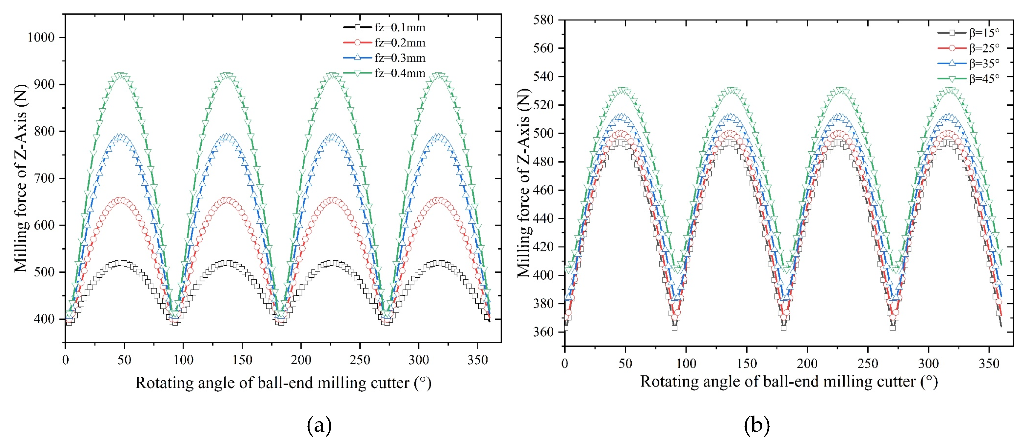
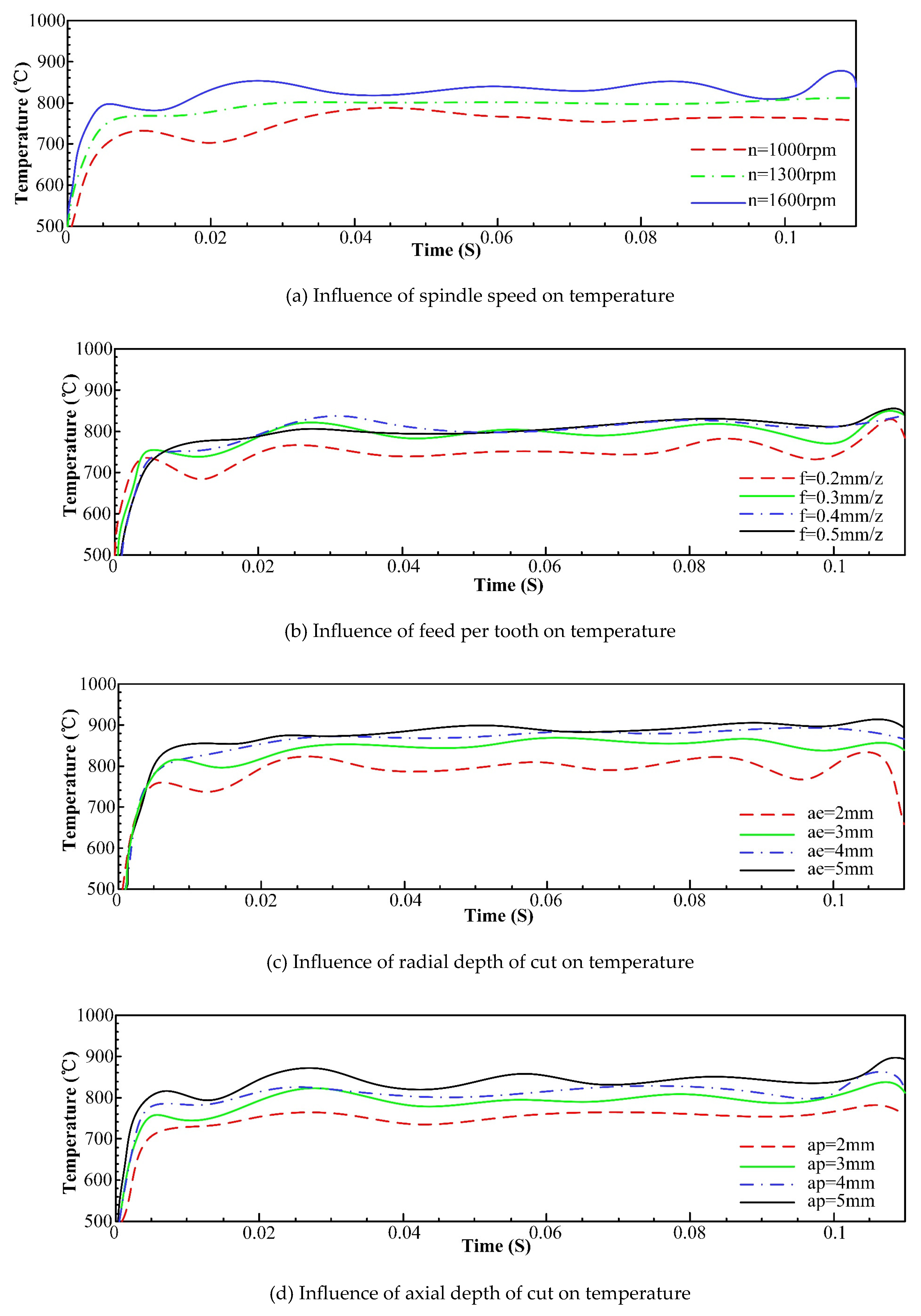
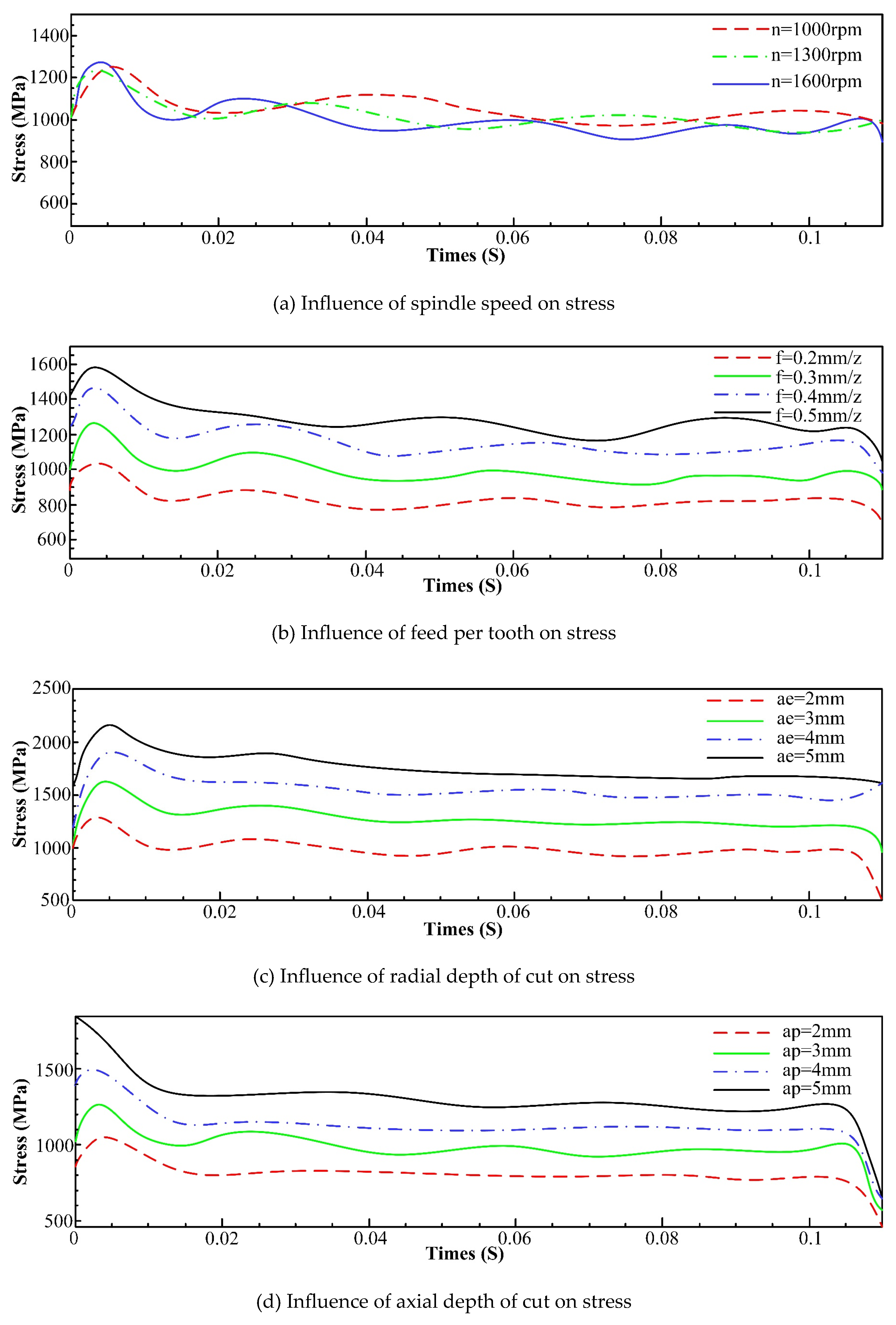
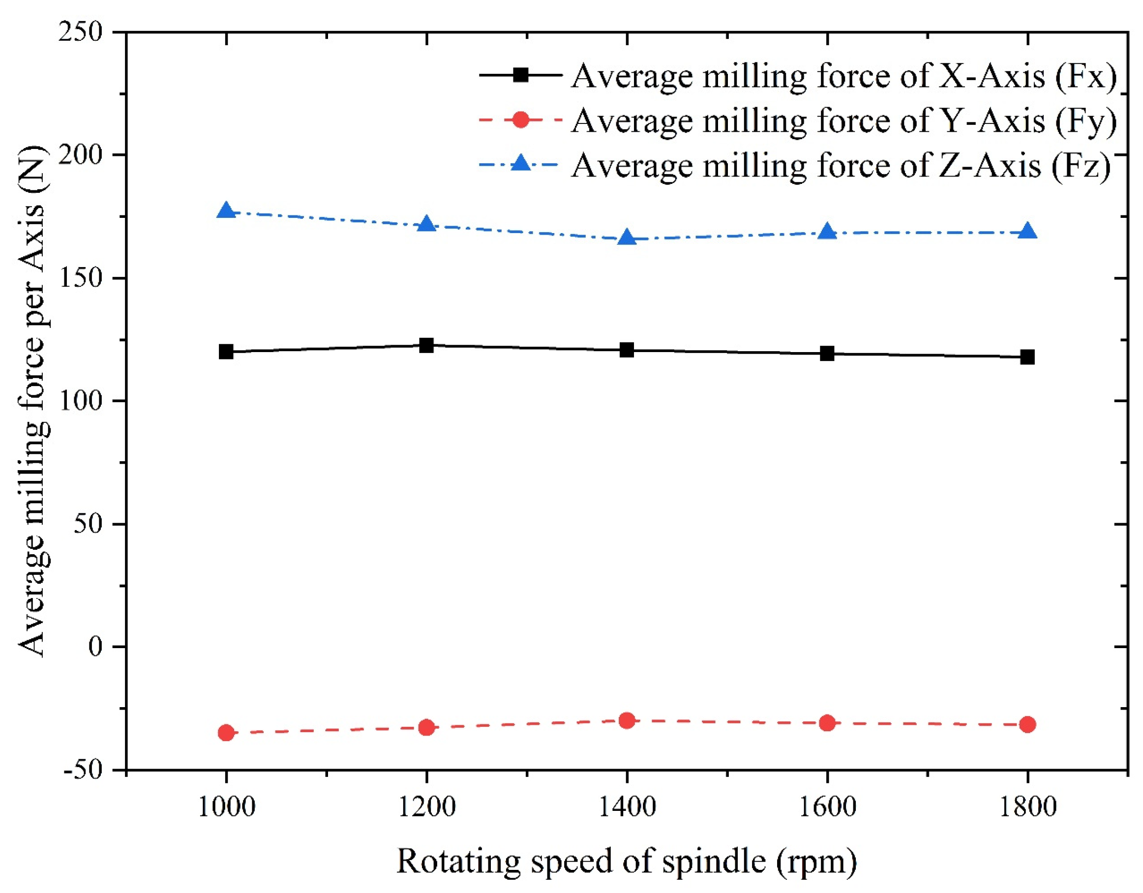
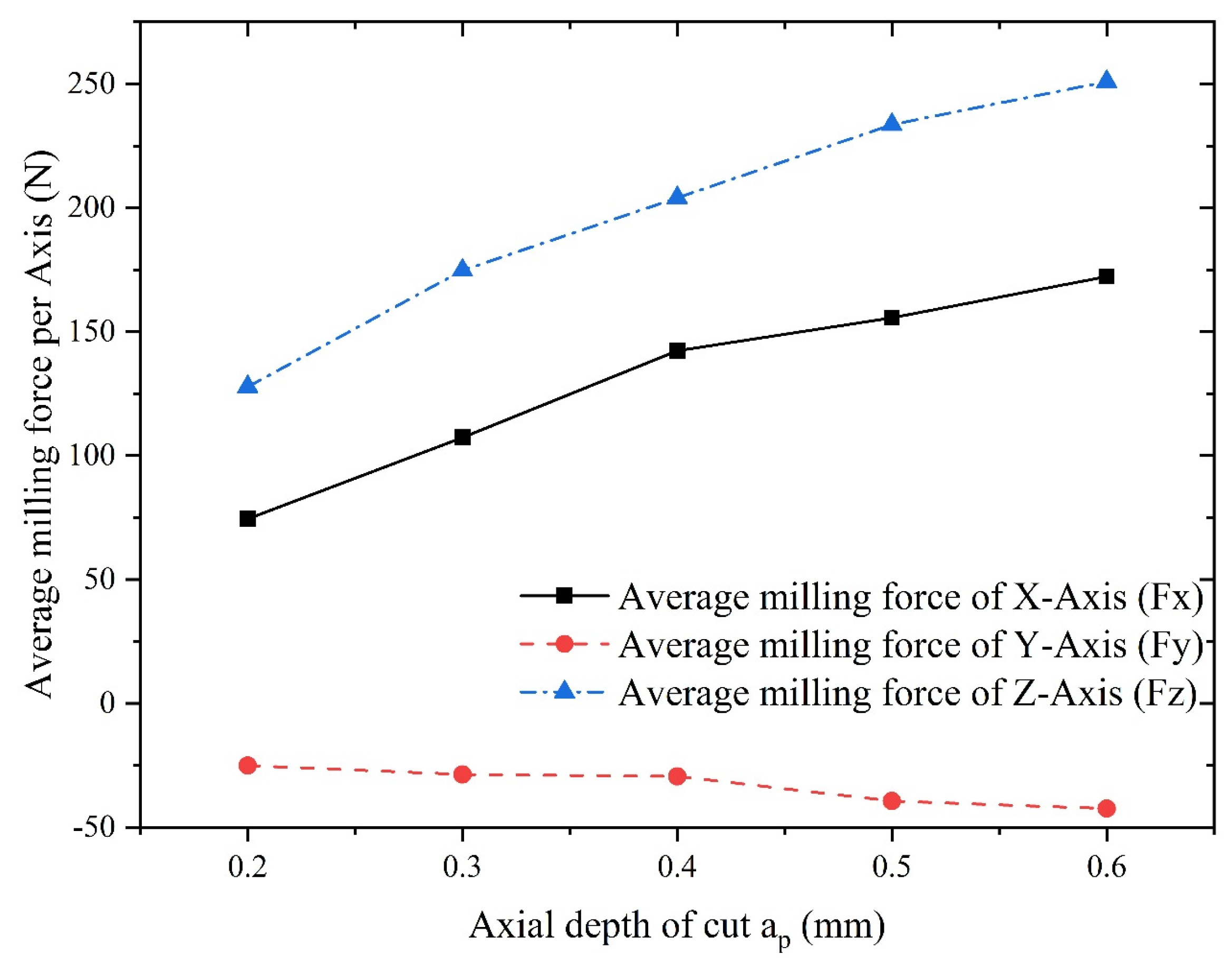
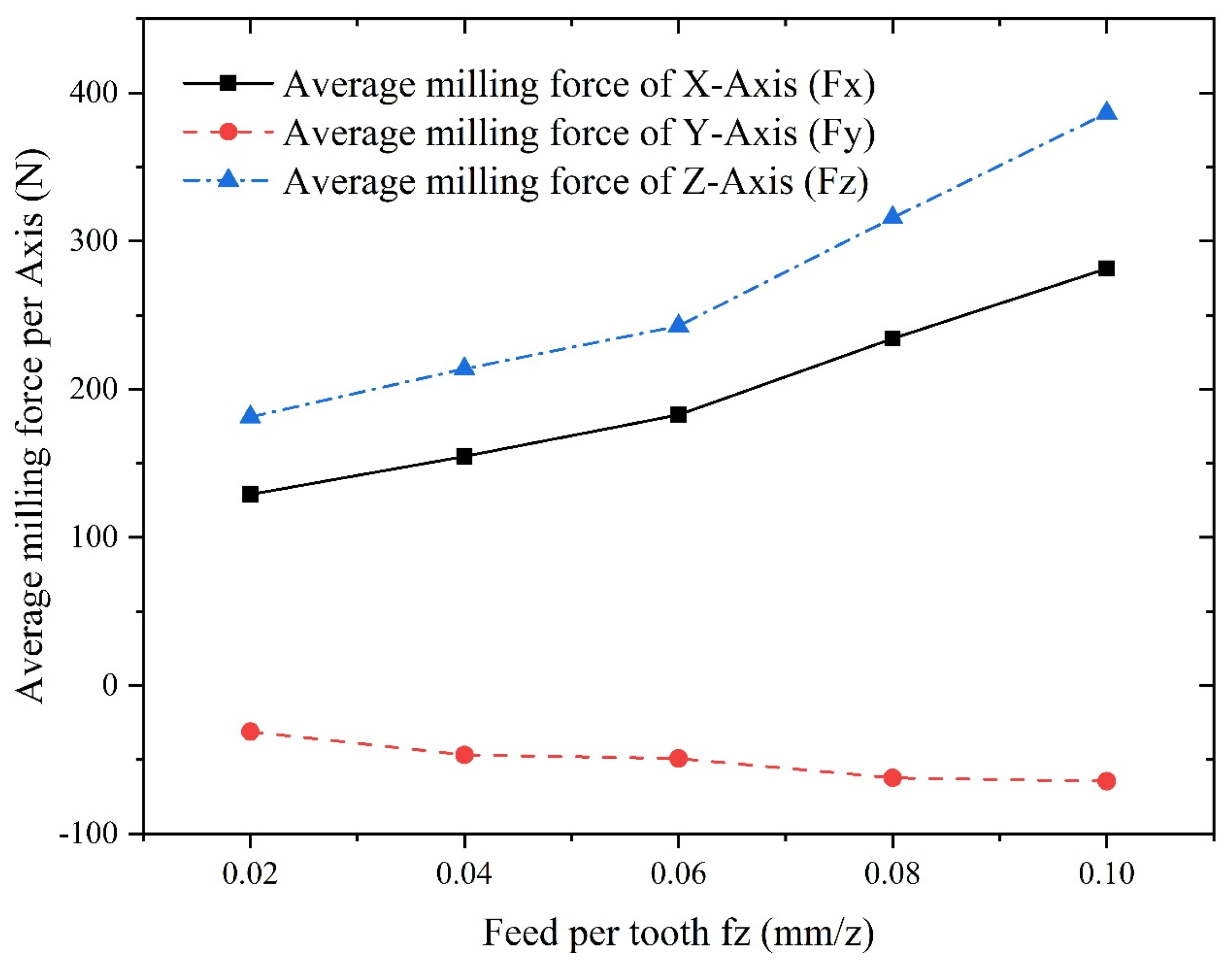
This paper takes Inconel718 as the research object, and carries out an in-depth discussion on the key problems in the process of machining Inconel718, specifically including milling force, milling temperature, milling stability, and optimization of processing parameters. The main conclusions are as follow:

An increase in feed and tool helix angle leads to an increase in milling force, and the results of finite element analysis indicate that with the increase of the spindle speed, radial depth of cut, axial depth of cut and feed per tooth, the increase of temperature in the machining area becomes more conspicuous. However, with the increase of spindle speed, the change of tool stress is not obvious, but with the increase of feed per tooth, radial depth of cut and axial depth of cut, the tool stress increases significantly. The spindle speed does not have a significant effect on the milling force in each axis. With the increase of feed per tooth and radial depth of cut, the milling force in X-, Y- and Z-Axis increases significantly, herein, the axial depth of cut has a greater effect on milling force of X-Axis and a smaller effect on milling forces of both Y- and Z-Axis.
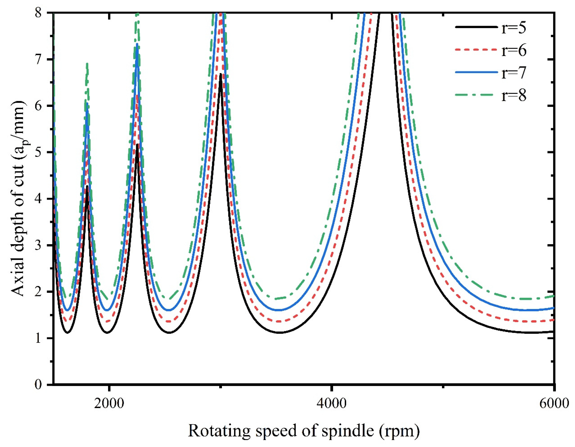
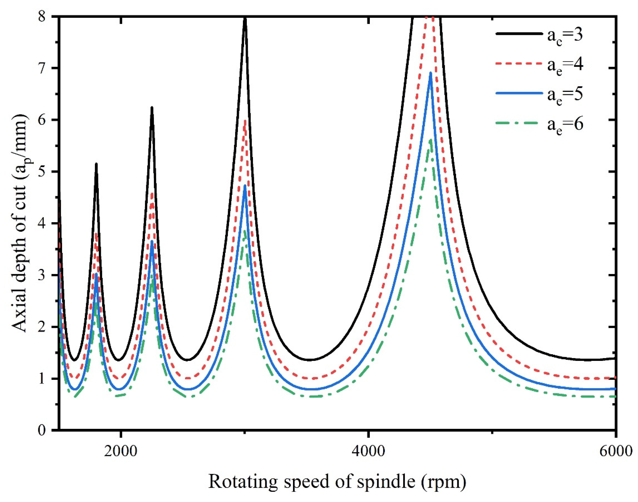
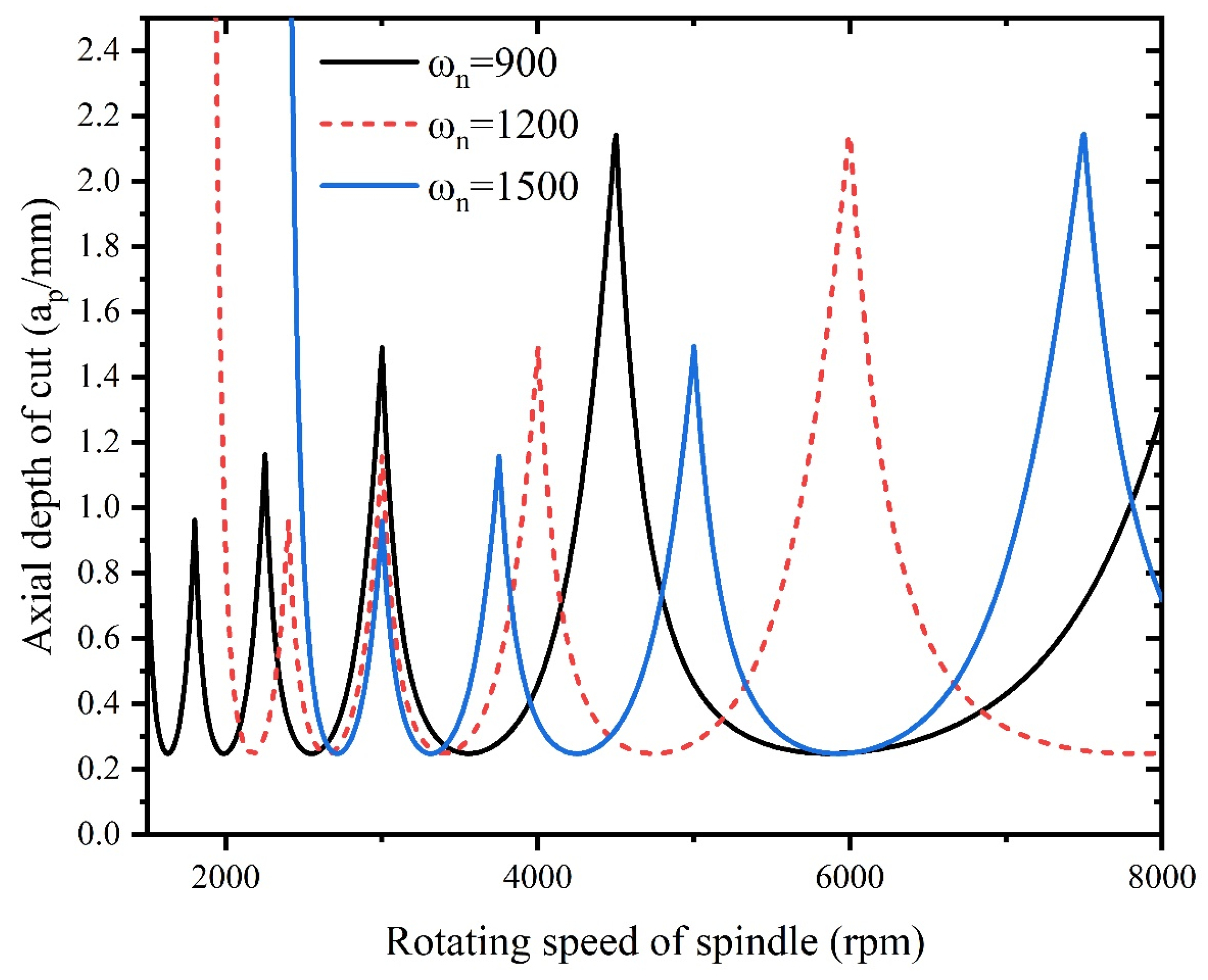
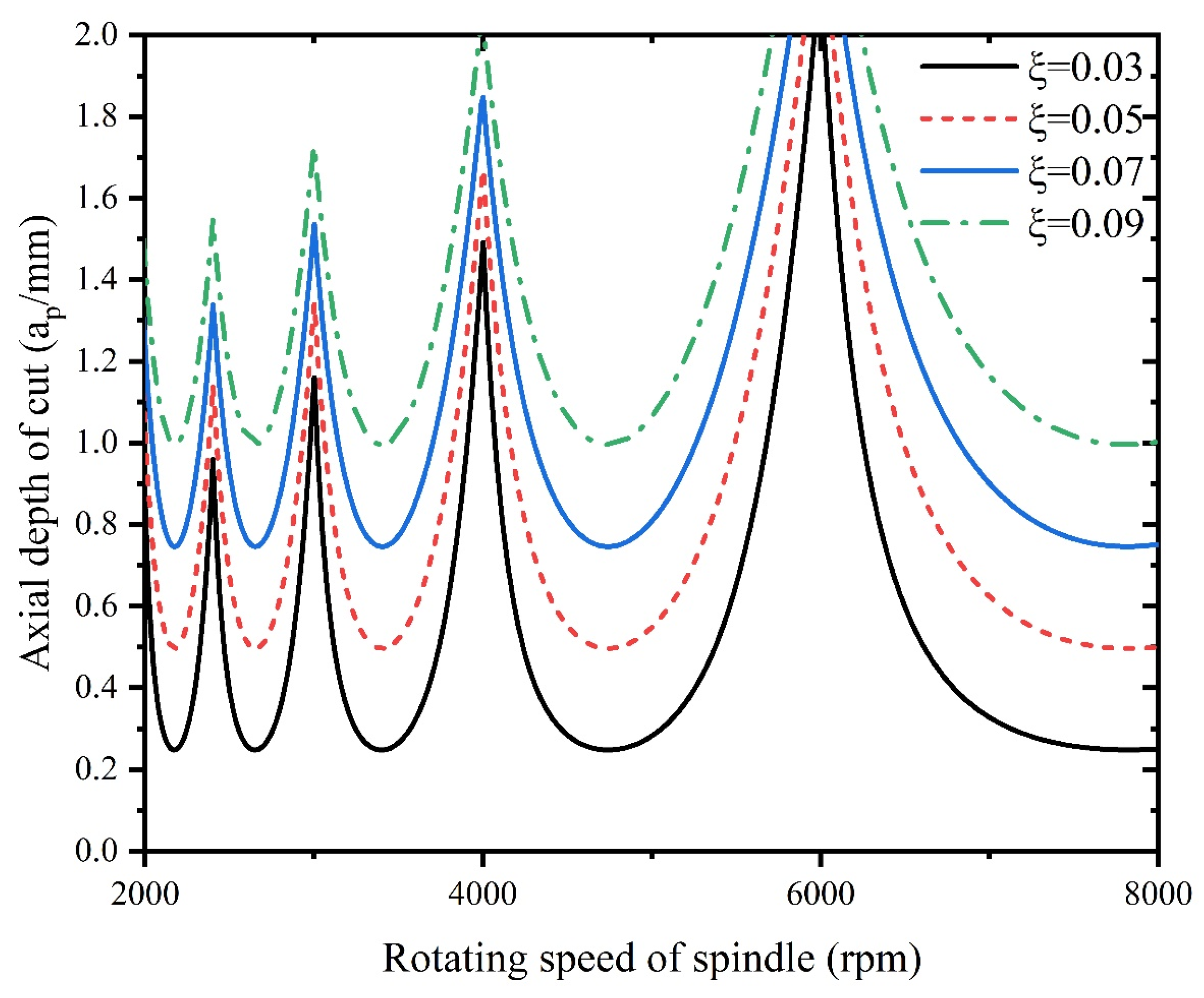
An increase in tool radius improves stability of milling system, however, an increase in radial depth of cut is detrimental to the stability. With increase of natural frequency, the critical depth of cut of milling remains unchanged, however, increase in damping ratio improves the system stability.
The order of influence on the average milling force in X-axis is: axial depth of cut > feed per tooth > spindle speed, and the order of influence on the average milling force in Y-axis is: spindle speed > feed per tooth > axial depth of cut.
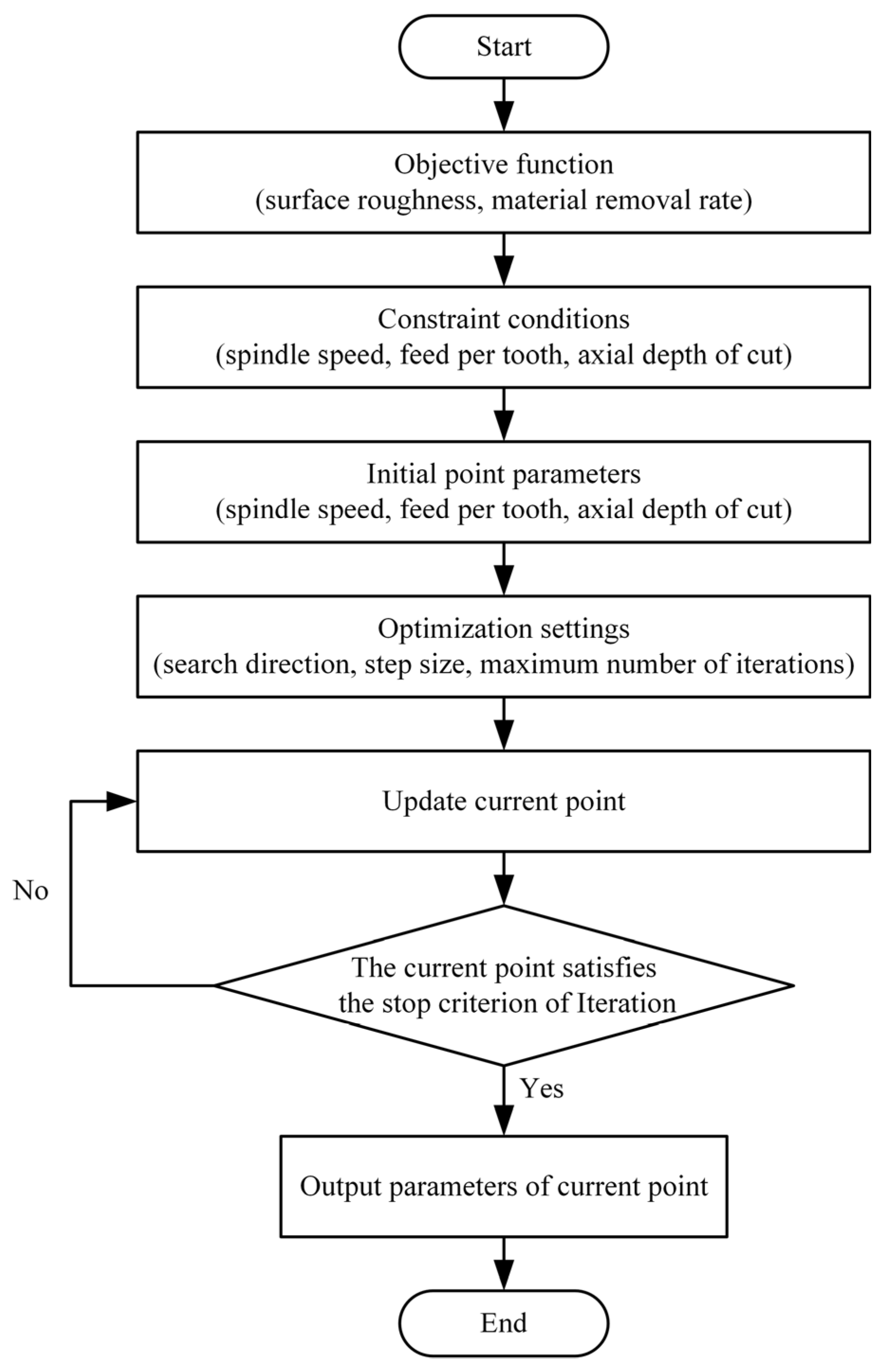
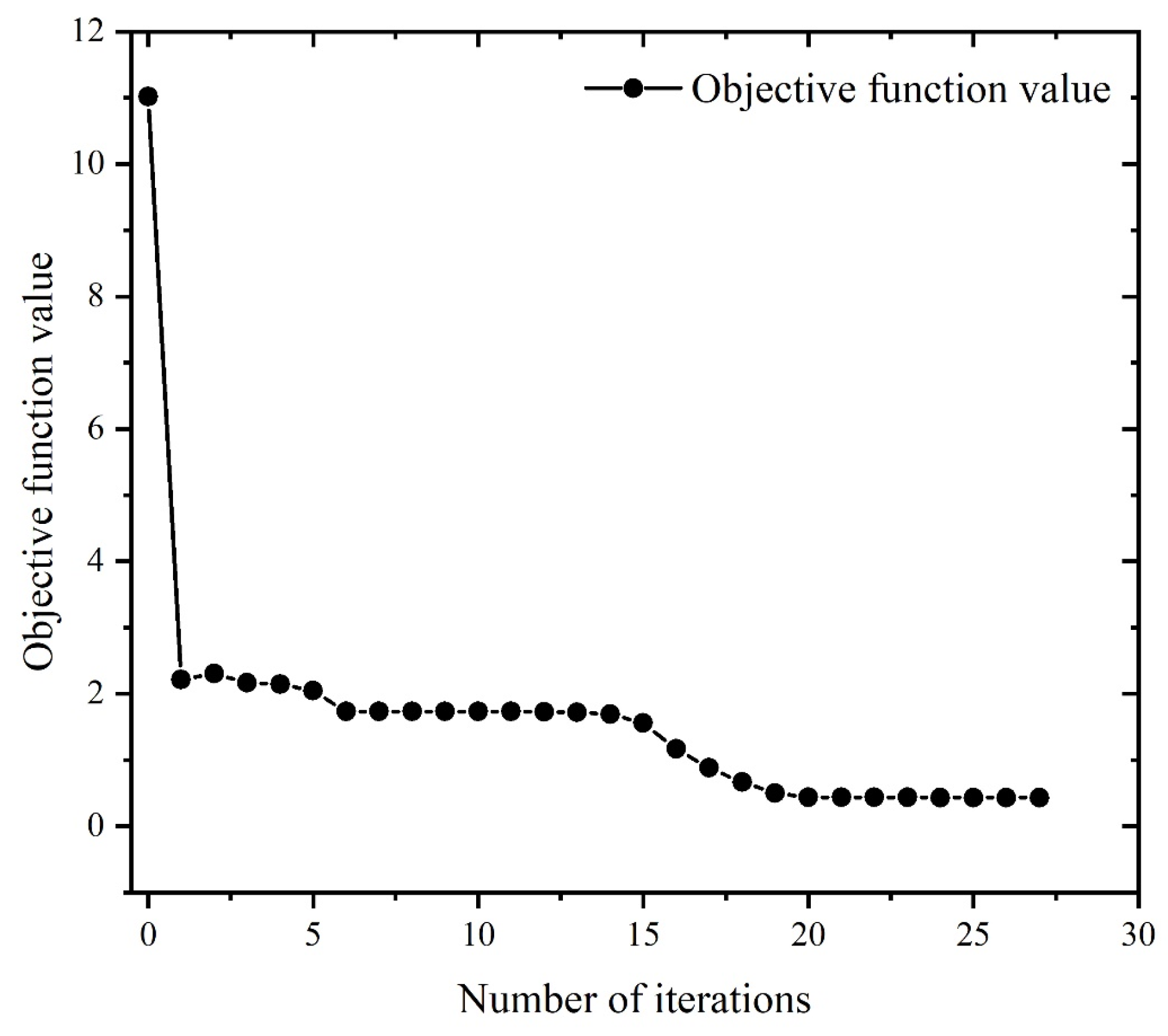
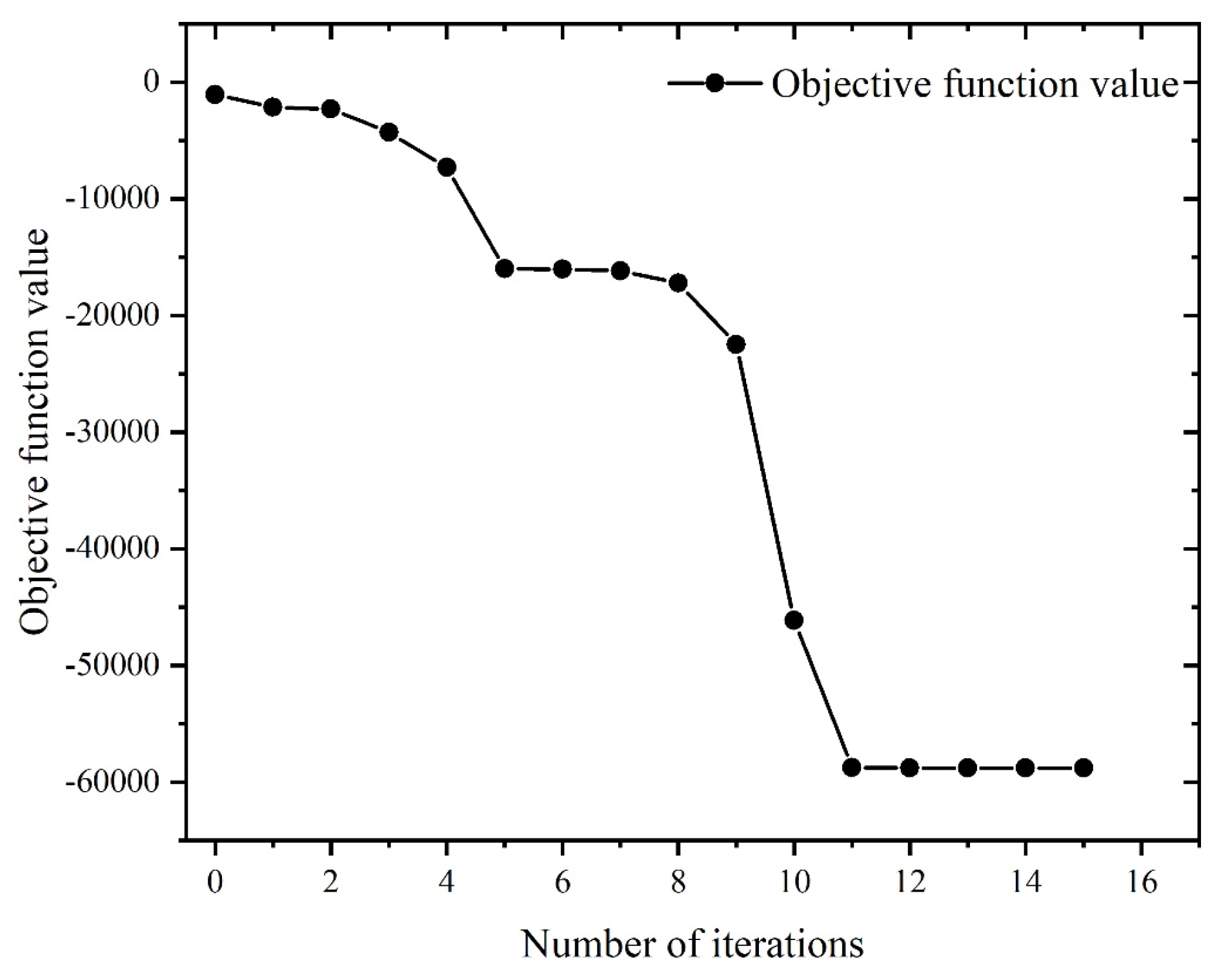
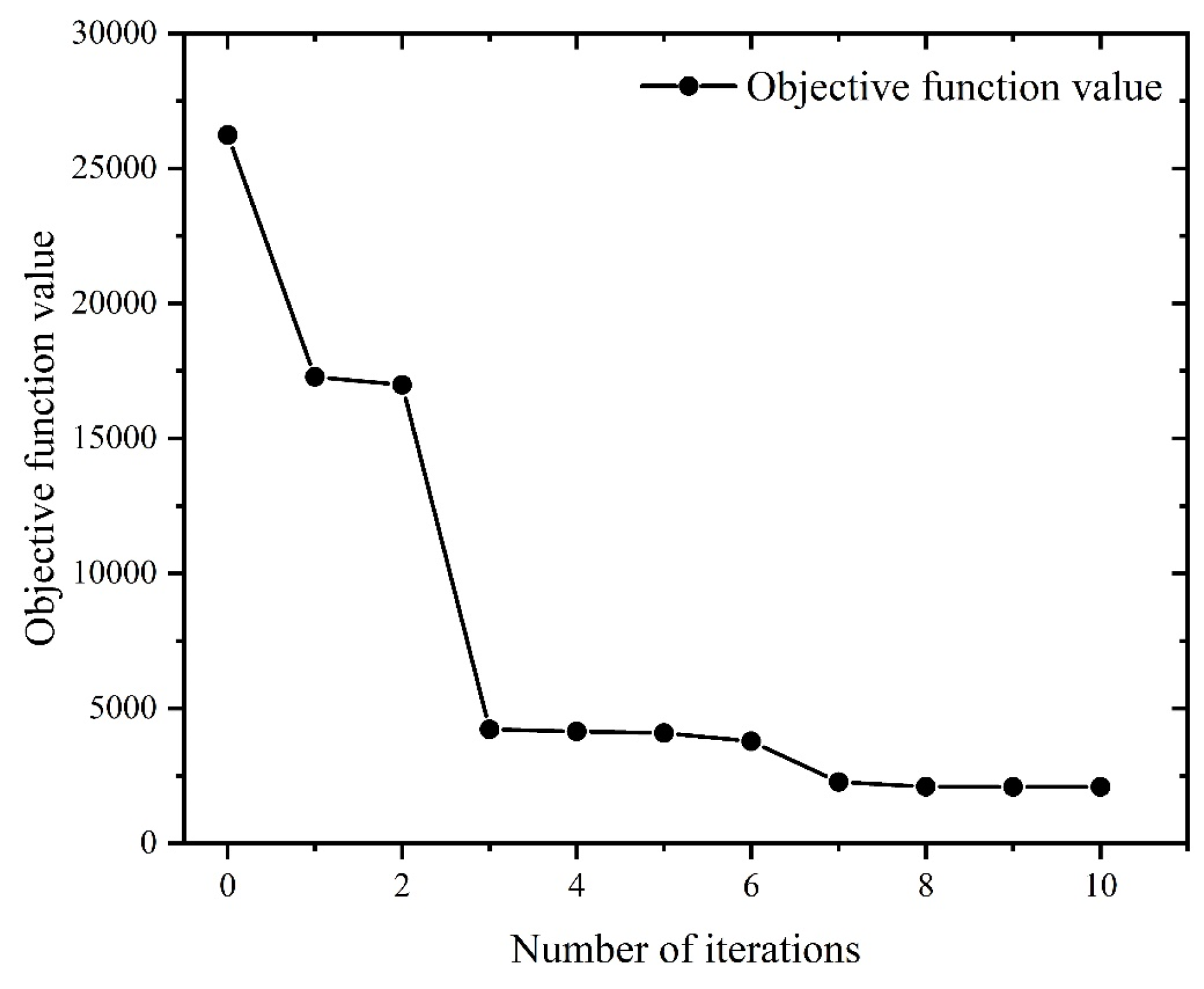
Using the fmincon algorithm, if the minimum surface roughness is considered as the optimization objective, the optimal machining parameters are: spindle speed 3999.63rpm, feed rate 80.01mm/min, axial depth of cut 0.25mm, at this time, the optimal value of surface roughness is 0.43 μm. If the maximum material removal rate is considered as the optimization objective, the optimal machining parameters are: spindle speed 4000rpm, feed speed 700mm/min, axial depth of cut 2.54mm, at this time, the optimal value of material removal rate is 58788.32mm³/min. If both the minimum surface roughness and maximum material removal rate are considered as the optimization objective, the optimal processing parameters are: spindle speed 3199.2rpm, feed speed 80mm/min, axial depth of cut 0.25mm. At this time, the value of surface roughness is 3.5 μm, and the value of material removal rate is 4199.2mm³/min.

Author Contributions

Conceptualization, J.Z. and H.Q.; methodology, J.Z.; software, H.Q.; validation, J.Z., Y.Z. and H.Q.; formal analysis, Y.Z.; investigation, J.Z.; resources, Y.Z.; data curation, Y.Z.; writing—original draft preparation, J.Z.; writing—review and editing, J.Z., Y.Z. and H.Q.; visualization, H.Q.; supervision, Y.Z.; project administration, Y.Z.; funding acquisition, Y.Z. All authors have read and agreed to the published version of the manuscript.

Funding

This research was funded by National Natural Science Foundation of China, grant number 62273081. This research was also funded by Liaoning Provincial Department of Education Scientific Research Funding Project, grant number LJKZ0001.

Institutional Review Board Statement

Not applicable.

Informed Consent Statement

Not applicable.

Data Availability Statement

Not applicable.

Conflicts of Interest

The authors declare no conflict of interest. The funders had no role in the design of the study; in the collection, analyses, or interpretation of data; in the writing of the manuscript; or in the decision to publish the results.

Appendix A

The nomenclature in this article is shown below:

$d F_{t, j} (ϕ_{j} (z))$	The differential tangential cutting force[N]
$d F_{r, j} (ϕ_{j} (z))$	The differential radial cutting force[N]
$d F_{a, j} (ϕ_{j} (z))$	The differential axial cutting force[N]
$K_{t c}$	Tangential shearing force coefficient[N/mm²]
$K_{r c}$	Radial shearing force coefficient[N/mm²]
$K_{a c}$	Axial shearing force coefficient[N/mm²]
$K_{t e}$	Tangential edge force coefficient[N/mm]
$K_{r e}$	Radial edge force coefficient[N/mm]
$K_{a e}$	Axial edge force coefficient[N/mm]
$h_{j} (ϕ_{j} (z))$	The instantaneous chip thickness at immersion angle[mm]
$d S (ϕ_{j} (z))$	The instantaneous edge length of the cutting segment[mm]
$d b$	The instantaneous chip width[mm]
$F_{f} (ϕ)$	The cutting force in feed direction[N]
$F_{n} (ϕ)$	The cutting force in normal direction[N]
$F_{z} (ϕ)$	The cutting force in axial direction[N]
$\bar{F_{f}}$	The average cutting force in the feed direction[N]
$\bar{F_{n}}$	The average cutting force in the normal direction[N]
$\bar{F_{z}}$	The average cutting force in the axial direction[N]
$\bar{F_{f c}}$ , $\bar{F_{f e}}$	The components of linear model force in the feed direction[N]
$\bar{F_{n c}}$ , $\bar{F_{n e}}$	The components of linear model force in the normal direction[N]
$\bar{F_{z c}}$ , $\bar{F_{z e}}$	The components of linear model force in the axial direction[N]
$σ (ε^{p}, \dot{ε}, T)$	Workpiece material flow stress
$g (ε^{p})$	Strain enhancement function
$Γ (\dot{ε})$	Strain rate effect function
$Θ (T)$	Thermal softening function
$\dot{ε}$	Strain rate
$T$	Temperature
$σ_{0}$	Initial yield stress
$ε^{p}$	Plastic strain
$ε_{0}^{p}$	Reference plastic strain
$ε_{c u t}^{p}$	Cut-off strain value
$n$	Contingency strengthening index
$Δ ε_{i}^{p}$	Instantaneous strain increment
$ε_{f_{i}}^{p}$	Material failure strain
$m_{x}$ , $m_{y}$	Mass of machine-tool system in X and Y direction
$c_{x}$ , $c_{y}$	Damping of machine-tool system in X and Y direction
$k_{x}$ , $k_{y}$	Stiffness of machine-tool system in X and Y direction
$F_{x j}$ , $F_{y j}$	Cutting force components acting on the tooth in X and Y direction
$v_{j, 0}$	Dynamic displacement of the cutter in the previous cycle
$v_{j}$	Dynamic displacement of the cutter in the current cycle
$g (ϕ_{j})$	Unit step function
$Φ_{x x} (i ω)$	Direct transfer function in X direction
$Φ_{y y} (i ω)$	Direct transfer function in Y direction
$Φ_{x y} (i ω)$	Cross-transfer function in X direction
$Φ_{y x} (i ω)$	Cross-transfer function in Y direction
$v_{c}$	Speed of milling process
$n$	Rotating speed of spindle
$f_{z}$	Feed per tooth
$a_{e}$	Radial depth of cut
$a_{p}$	Axial depth of cut

Appendix B

The Matlab program used to solve milling force model of the ball-end milling cutter is shown below:

clear;

clc;

R=4;

%ap=0.2;

zt1=-R:0.01:0;

phi_2=linspace(0,2*pi,100);

n11=1;

%Cutter Parameters

beta=45/180*pi;D=10;Nf=2;R=D/2;

%Cutting Parameters

ap=0.2;fz=0.1;n=1200;

%Coefficient of Milling Force

Kts=3304.12;

Krs=2148.90;

Kas=725.07;

Kre=67.58;

Kte=5.28;

Kae=-7.16;

%Differential Elements

dphi=0.01;dz=0.01;

K=700;

dphi=4*pi/K;

zt1=-R:dz:0;

phi_p=2*pi/Nf;wr=2*pi*n/60;

for m=1:K%Discretization of rotating angle

phi(m)=m*dphi;

Fx(m)=0;Fy(m)=0;Fz(m)=0;

dFx=0;dFy=0;dFz=0;

for k=1:2%Number of teeth cycle

phi_11=phi(m)+(k-1)*phi_p;%Rotation angle considering the number of teeth

for i=2:length(zt1)

z=zt1(i);

zt=z;

phi_3=phi_11-(z+R)*tan(beta)/R;

ks=acos(-zt/R);

if mod(phi_3,2*pi)>=0& mod(phi_3,2*pi)<=pi

dS=sqrt(1+z^2/(R^2-z^2)+tan(beta)^2/R^2*(R^2-z^2))*dz;

db=R/(R^2-z^2)*dz;

%Calculation of cutting thickness

tn=fz*sin(phi_3)*sin(ks);

%End of calculation of cutting thickness

k1=acos(-z/R);

dFr=Kre*dS+Krs*tn*db;

dFt=Kte*dS+Kts*tn*db;

dFa=Kae*dS+Kas*tn*db;

dFx=-cos(phi_3)*dFt-sin(k1)*sin(phi_3)*dFr-cos(k1)*sin(phi_3)*dFa;

dFy=sin(phi_3)*dFt-sin(k1)*cos(phi_3)*dFr-cos(k1)*cos(phi_3)*dFa;

dFz=cos(k1)*dFr-sin(k1)*dFa;

else

dFx=0;

dFy=0;

dFz=0;

end

Fx(m)=Fx(m)+dFx;

Fy(m)=Fy(m)+dFy;

Fz(m)=Fz(m)+dFz;

end

phi_x=phi/pi*180/2;

plot(phi_x,Fx,'r','MarkerSize',3,'LineWidth',2);

hold on;

plot(phi_x,Fy,'b','MarkerSize',3,'LineWidth',2);

hold on;

plot(phi_x,Fz,'k','MarkerSize',3,'LineWidth',2);

hold on;

set(gca,'linewidth',0.5,'fontsize',15,'fontname','Times');

References

Zhou, Y.; Ma, L.; Gong, Y.; Zhang, L.; Yin, G.; Sun, Y.J.T.I.J.o.A.M.T. Study on the mechanism of chip forming and the microhardness of micro-grinding nickel-based single-crystal superalloy. 2019, 103, 281–295. [Google Scholar] [CrossRef]
Thellaputta, G.R.; Chandra, P.S.; Rao, C.S.P. Machinability of Nickel Based Superalloys: A Review. Materials Today: Proceedings 2017, 4, 3712–3721. [Google Scholar] [CrossRef]
Miller, S. Advanced materials mean advanced engines. Interdisciplinary Science Reviews 1996, 21, 117–129. [Google Scholar] [CrossRef]
Ezugwu, E.O.; Wang, Z.M.; Machado, A.R. The machinability of nickel-based alloys: a review. Journal of Materials Processing Technology 1999, 86, 1–16. [Google Scholar] [CrossRef]
Ge, Y.; Zhu, Z.; Wang, D. Electrochemical Dissolution Behavior of the Nickel-Based Cast Superalloy K423A in NaNO3 Solution. Electrochimica Acta 2017, 253, 379–389. [Google Scholar] [CrossRef]
Alabort, E.; Reed, R.C.; Barba, D. Combined modelling and miniaturised characterisation of high-temperature forging in a nickel-based superalloy. Materials & Design 2018, 160, 683–697. [Google Scholar] [CrossRef]
Xu, D.; Liao, Z.; Axinte, D.; Sarasua, J.A.; M'Saoubi, R.; Wretland, A. Investigation of surface integrity in laser-assisted machining of nickel based superalloy. Materials & Design 2020, 194, 108851. [Google Scholar] [CrossRef]
Sharma, P.; Kishore, K.; Sinha, M.K.; Singh, V. Electrical discharge machining of nickel-based superalloys: a comprehensive review. International Journal of Materials Engineering Innovation 2022, 13, 157–190. [Google Scholar] [CrossRef]
Ezugwu, E.O.; Bonney, J.; Yamane, Y. An overview of the machinability of aeroengine alloys. Journal of Materials Processing Technology 2003, 134, 233–253. [Google Scholar] [CrossRef]
Ding, T.; Zhang, S.; Wang, Y.; Zhu, X.J.T.I.J.o.A.M.T. Empirical models and optimal cutting parameters for cutting forces and surface roughness in hard milling of AISI H13 steel. 2010, 51, 45–55.
Zhao, C.; Fu, T.; Liu, Y.; Guo, Y.J.I.J.I.T. Different Impact on the Stability Limits Caused by the Selection of Milling Force Coefficient under the State of High-Speed Milling. 2015, 8, 153–160. [Google Scholar] [CrossRef]
Shi, L.; Liu, E.F.; Zhang, Y.; Chen, P.; Li, Z.B. The simulation of cutting force of free-form surface machining with ball-end milling cutter. In Proceedings of the 2009 IEEE International Conference on Industrial Engineering and Engineering Management; 2009; pp. 2314–2318. [Google Scholar]
Bergmann, J.A.; Wöste, F.; Wiederkehr, P. An analysis of the sensitivity of cutting force coefficients and their influence on the variability of stability diagrams. Production Engineering 2023, 17, 407–414. [Google Scholar] [CrossRef]
Zhao, M.; Zhu, J.; Song, S.; Xue, B.; Zhao, B. Influence of machining parameters in longitudinal-torsional ultrasonic vibration milling titanium alloy for milling force. The International Journal of Advanced Manufacturing Technology 2022, 123, 3587–3597. [Google Scholar] [CrossRef]
Newby, G.; Venkatachalam, S.; Liang, S.Y. Empirical analysis of cutting force constants in micro-end-milling operations. Journal of Materials Processing Technology 2007, 192-193, 41–47. [Google Scholar] [CrossRef]
Li, X.; Wang, Y.; Miao, L.; Zhang, W. Deformation Analysis of Continuous Milling of Inconel718 Nickel-Based Superalloy. Micromachines 2022, 13. [Google Scholar] [CrossRef] [PubMed]
Jiang, F.; Zhang, T.; Yan, L. Analytical model of milling forces based on time-variant sculptured shear surface. International Journal of Mechanical Sciences 2016, 115-116, 190–201. [Google Scholar] [CrossRef]
Madajewski, M.; Wojciechowski, S.; Znojkiewicz, N.; Twardowski, P. Hybrid Numerical-Analytical Approach for Force Prediction in End Milling of 42CrMo4 Steel. In Proceedings of the Advances in Manufacturing II, Cham, 2019; 2019//; pp. 223–232. [Google Scholar]
Huang, W.; Li, X.; Wang, B.; Chen, J.; Zhou, J. An analytical index relating cutting force to axial depth of cut for cylindrical end mills. International Journal of Machine Tools and Manufacture 2016, 111, 63–67. [Google Scholar] [CrossRef]
Kao, Y.-C.; Nguyen, N.-T.; Chen, M.-S.; Huang, S.-C. A combination method of the theory and experiment in determination of cutting force coefficients in ball-end mill processes. Journal of Computational Design and Engineering 2015, 2, 233–247. [Google Scholar] [CrossRef]
Zhou, Z.; Wang, H.J.T.I.J.o.A.M.T. Full life-cycle cutting force prediction in ball helical milling based on oblique cutting analysis. 2023, 124, 1623–1638. [Google Scholar] [CrossRef]
Kaneko, K.; Nishida, I.; Sato, R.; Shirase, K.J.P.C. Virtual milling force monitoring method based on in-process milling force prediction model to eliminate predetermination of cutting coefficients. 2018, 77, 22–25. [Google Scholar] [CrossRef]
Li, S.-J.; Zhou, Y.-F.; Jin, R.-C.; Ji, Z. Dynamic Force Modelling for a Ball-End Milling Cutter Based on the Merchant Oblique Cutting Theory. The International Journal of Advanced Manufacturing Technology 2001, 17, 477–483. [Google Scholar] [CrossRef]
Falta, J.; Sulitka, M.; Zeman, P.J.T.I.J.o.A.M.T. An analytical formulation of ZOA-based machining stability for complex tool geometries: application to 5-axis ball-end milling. 2022, 123, 1499–1519. [Google Scholar] [CrossRef]
Yongheng, D.; Shujuan, L.; Xiantao, H.; Pengyang, L.; Yan, L.; Qi, L.J.C.J.M.E. Modeling on the milling force of ball-end milling cutter based on Z-MAP method. 2019, 55, 201–212. [Google Scholar] [CrossRef]
Huang, S.; Liu, Y.; Jiao, K.; Li, J. Three-dimensional finite element simulation analysis of milling deformation of SiCp/Al composites thin-walled parts. International Journal of Machining and Machinability of Materials 2017, 19, 408–425. [Google Scholar] [CrossRef]
Yu, J.; Shi, Y.X.; Yang, G.W. Finite Element Analysis and Experimental of Milling Force for Aeronautical Thin-Walled Workpiece. Advanced Materials Research 2011, 328-330, 685–689. [Google Scholar] [CrossRef]
Haijun, H.; Yazhou, S.; Zesheng, L. Simulation and experiment of cutting force in ultrasonic torsional vibration assisted micro-milling. In Proceedings of the Proc.SPIE; 2010; p. 76570. [Google Scholar]
Pratap, T.; Patra, K.; Dyakonov, A.A.J.P.E. Modeling cutting force in micro-milling of Ti-6Al-4V titanium alloy. 2015, 129, 134–139. [Google Scholar] [CrossRef]
Li, M.-Y.; Ding, W.-B.; Yu, H.-B.; Huang, J.-G. RESEARCH ON DEFORMATION CHARACTERISTICS OF RULED SURFACE BLADES IN MILLING PROCESSES. In Material Engineering and Mechanical Engineering: Proceedings of Material Engineering and Mechanical Engineering (MEES2015); pp. 2016910–919.
Altintaş, Y.; Budak, E.J.C.a. Analytical prediction of stability lobes in milling. 1995, 44, 357–362. [Google Scholar] [CrossRef]
Merdol, S.; Altintas, Y.J.J.M.S.E. Multi frequency solution of chatter stability for low immersion milling. 2004, 126, 459–466. [Google Scholar] [CrossRef]
Ding, Y.; Zhu, L.; Zhang, X.; Ding, H. Second-order full-discretization method for milling stability prediction. International Journal of Machine Tools and Manufacture 2010, 50, 926–932. [Google Scholar] [CrossRef]
Ding, Y.; Zhu, L.; Zhang, X.; Ding, H.J.I.J.o.M.T. ; Manufacture. A full-discretization method for prediction of milling stability. 2010, 50, 502–509. [Google Scholar]
Insperger, T.; Stépán, G.; Turi, J.J.J.o.S. ; Vibration. On the higher-order semi-discretizations for periodic delayed systems. 2008, 313, 334–341. [Google Scholar]
Insperger, T.; Stépán, G.J.I.J.f.n.m.i.e. Semi-discretization method for delayed systems. 2002, 55, 503–518. [Google Scholar] [CrossRef]
Insperger, T.; Stépán, G.J.I.j.f.n.m.i.e. Updated semi-discretization method for periodic delay-differential equations with discrete delay. 2004, 61, 117–141. 2004, 61, 117–141. [Google Scholar]
Sun, L.; Zheng, K.; Liao, W. Chatter suppression and stability analysis of rotary ultrasonic milling titanium alloy thin-walled workpiece. The International Journal of Advanced Manufacturing Technology 2022, 118, 2193–2204. [Google Scholar] [CrossRef]
Liu, S.; Zhang, J.F.; Feng, P.F.; Yu, D.W.; Wu, Z.J. Determination of Constitutive Equation Parameters for Face Milling 3-D Simulation via Pressure Bar and Orthogonal Cutting Tests. Materials Science Forum 2012, 723, 136–142. [Google Scholar] [CrossRef]
Li, B.; Hu, Y.; Wang, X.; Li, C.; Li, X. AN ANALYTICAL MODEL OF OBLIQUE CUTTING WITH APPLICATION TO END MILLING. Machining Science and Technology 2011, 15, 453–484. [Google Scholar] [CrossRef]
Tao, F. The Experiment of Cutting Performance of Polished Cemented Carbide Insert in Cutting Nickel-Based Superalloy. Xiangtan University, 2017.

Figure 1. Milling force model of ball-end milling cutter.

Figure 2. The relationship between average milling force and feed per tooth.

Figure 3. Experimental and theoretical comparison of milling forces.

Figure 4. Influence of processing parameters on milling force of X-Axis: (a) Influence of feed per tooth; (b) Influence of tool helix angle.

Figure 5. Influence of processing parameters on milling force of Y-Axis: (a) Influence of feed per tooth; (b) Influence of tool helix angle.

Figure 6. Influence of processing parameters on milling force of Z-Axis: (a) Influence of feed per tooth; (b) Influence of tool helix angle.

Figure 7. Finite element model of tool and workpiece.

Figure 8. Influence of processing parameters on temperature.

Figure 9. Influence of machining parameters on stress.

Figure 10. Comparison of simulation and theoretical milling forces: (a) Milling force of FEM Simulation; (b) Theoretical milling force.

Figure 11. Comparison of milling forces of each axis at different spindle speeds.

Figure 12. Comparison of milling forces of each axis at different feed per tooth.

Figure 13. Comparison of milling forces of various axis under different radial depth of cut.

Figure 14. Comparison of milling forces of different axis under different axial depth of cut.

Figure 15. Dynamic model of machine-tool system.

Figure 16. Dynamic changes of cutting thickness.

Figure 17. Schematic diagram of equipment connection of modal experiment.

Figure 18. Photo of equipment connection of modal experiment.

Figure 19. Distribution of measuring points of tool.

Figure 20. Tool modal of X direction.

Figure 21. Tool modal of Y direction.

Figure 22. Figure 22. Influence of tool radius on stability.

Figure 23. Influence of radial depth of cut on stability.

Figure 24. Influence of natural frequency on stability.

Figure 25. Influence of damping ratio on stability.

Figure 26. Schematic diagram of connection of experimental equipment.

Figure 27. Device connection diagram.

Figure 28. Influence of spindle speed on average milling force of each axis.

Figure 29. Influence of axial depth of cut on average milling force of each axis.

Figure 30. Influence of feed per tooth on average milling force of each axis.

Figure 31. Flowchart of procedure of optimization using fmincon algorithm.

Figure 32. Iteration curve of surface roughness.

Figure 33. Iterative curve of material removal rate.

Figure 34. Multi-objective optimization iteration curve.

Table 1. Data of recognition experiments of milling force coefficient.

Experiment No.	$f_{t}$ (mm/z)	Feed speed (mm/min)	$\bar{F_{x}} (N)$	$\bar{F_{y}} (N)$	$\bar{F_{z}} (N)$
1	0.02	80	76.88	-59.25	11.97
2	0.04	160	174.5	-210.7	44.67
3	0.06	240	251.7	-378.8	133.1
4	0.08	320	314.1	-572.0	265.2
5	0.10	400	353.4	-720.6	430.1
6	0.12	480	421.6	-830.1	552.3

Table 2. Milling force coefficients.

Shearing force coefficient (N/mm²)	Value	Edge force coefficient (N/mm²)	Value
$K_{t c}$	-15934.72	$K_{t e}$	149.15
$K_{r c}$	-6636.28	$K_{r e}$	-51.95
$K_{a c}$	8949.06	$K_{a e}$	-159.45

Table 3. Strain enhancement parameters of Inconel718.

Initial yield stress $σ_{0}$	Reference plastic strain $ε_{0}^{p}$	Cut-off strain $ε_{c u t}^{p}$	Strain enhancement index n
3.6 MPa	$5.228 \times 10^{- 3}$	0.3	9.55

Table 4. Thermal softening parameters of Inconel718.

$c_{0}$	$c_{1}$	$c_{2}$	$c_{3}$	$c_{4}$	$c_{5}$	Ambient Temperature $T$	Linear cut-off temperature $T_{c u t}$	Melting Temperature $T_{m e l t}$
0.998	$2.46 \times 10^{- 4}$	$- 3.74 \times 10^{- 6}$	$1.51 \times 10^{- 8}$	$- 2.35 \times 10^{- 11}$	$1.10 \times 10^{- 14}$	$20^{°} C$	$1050^{°} C$	$1298^{°} C$

Table 5. Strain rate parameters of Inconel718.

Low strain rate sensitivity factor $m_{1}$	High strain rate sensitivity factor $m_{2}$	Reference plastic strain rate ${\dot{ε}}_{0}$	Strain rate critical value ${\dot{ε}}_{t}$
25.5	25.5	1 sec-1	1×107 sec-1

Table 6. Processing parameters used in finite element analysis.

Rotating speed of spindle n(rpm)	Feed per tooth $f_{t}$ (mm/z)	Radial depth of cut $a_{e}$ (mm)	Axial depth of cut $a_{p}$ (mm)
1000	0.2	2	2
1300	0.3	3	3
1600	0.4	4	4
-	0.5	5	5

Table 7. Results of modal experiments.

Modal order	Natural frequency (Hz)	Damping ratio (%)
First order of X direction	935.06	0.049
Second order of X direction	1235.96	0.036
Third order of X direction	1567.99	0.093
First order of Y direction	911.87	0.045
Second order of Y direction	1233.52	0.059
Third order of Y direction	1539.92	0.050

Table 8. Parameter of single factor experiments.

Experiment No.	Rotating speed of spindle n(r/min)	Feed per tooth $f_{z}$ (mm/z)	Axial depth of cut $a_{p}$ (mm)
1	1000/1200/1400/1600/1800	0.02	0.4
2	1000	0.02/0.04/0.06/0.08/0.10	0.4
3	1000	0.02	0.2/0.3/0.4/0.5/0.6

Table 9. Parameter of orthogonal experiments.

Experiment No.	Rotating speed of spindle n(rpm)	Feed per tooth $f_{z}$ (mm/z)	Axial depth of cut $a_{p}$ (mm)
1	800	0.015	0.1
2	800	0.03	0.2
3	800	0.045	0.3
4	800	0.06	0.4
5	1000	0.015	0.2
6	1000	0.03	0.1
7	1000	0.045	0.4
8	1000	0.06	0.3
9	1200	0.015	0.3
10	1200	0.03	0.4
11	1200	0.045	0.1
12	1200	0.06	0.2
13	1400	0.015	0.4
14	1400	0.03	0.3
15	1400	0.045	0.2
16	1400	0.06	0.1

Table 10. Result of orthogonal experiments.

Experiment No.	Parameters of experiment			Result of experiment(N)
Experiment No.	Rotating speed of spindle n(rpm)	Feed per tooth $f_{z}$ (mm/z)	Axial depth of cut $a_{p}$ (mm)	$\bar{F_{x}}$	$\bar{F_{y}}$	$\bar{F_{z}}$	$\bar{F}$
1	800	0.015	0.1	15.81	8.410	25.53	31.18
2	800	0.03	0.2	49.01	-7.847	68.23	84.37
3	800	0.045	0.3	85.91	-18.33	107.4	138.75
4	800	0.06	0.4	131.0	-28.87	137.0	191.74
5	1000	0.015	0.2	57.65	-15.96	87.60	106.08
6	1000	0.03	0.1	39.64	-8.765	65.59	77.14
7	1000	0.045	0.4	58.2	42.99	70.62	101.11
8	1000	0.06	0.3	118.4	-13.09	148.7	190.53
9	1200	0.015	0.3	79.75	-16.09	117.9	143.25
10	1200	0.03	0.4	121.9	-24.2	157.3	200.47
11	1200	0.045	0.1	38.06	-9.168	66.27	76.97
12	1200	0.06	0.2	53.36	35.24	69.54	94.47
13	1400	0.015	0.4	86.23	2.896	120.7	148.37
14	1400	0.03	0.3	54.12	40.37	82.35	106.49
15	1400	0.045	0.2	87.04	-23.66	134.8	162.19
16	1400	0.06	0.1	66.65	-12.69	101.1	121.76

Table 11. Comparison between theoretical and experimental results of milling force.

Experiment No.	Milling force	Theoretical result (N)	Experimental result (N)	Relative error (%)
1	$F_{x}$	17.86	15.81	12.97
	$F_{y}$	9.46	8.41	12.49
	$F_{z}$	27.74	25.53	8.66
2	$F_{x}$	55.68	49.01	13.61
	$F_{y}$	8.64	7.847	10.11
	$F_{z}$	59.96	68.23	12.12
3	$F_{x}$	80.36	85.91	6.46
	$F_{y}$	19.99	18.33	9.06
	$F_{z}$	97.27	107.4	9.43
4	$F_{x}$	144.22	131	10.09
	$F_{y}$	30.74	28.87	6.48
	$F_{z}$	123.98	137	9.50

Table 12. Comparison between theoretical and finite element analysis results of milling force.

Experiment No.	Milling force	FEA result (N)	Experimental result (N)	Relative error (%)
1	$F_{x}$	13.63	15.81	13.80
	$F_{y}$	7.25	8.41	13.79
	$F_{z}$	23.28	25.53	8.81
2	$F_{x}$	46.93	49.01	4.24
	$F_{y}$	8.63	7.847	9.98
	$F_{z}$	75.02	68.23	9.95
3	$F_{x}$	91.02	85.91	5.95
	$F_{y}$	16.97	18.33	7.42
	$F_{z}$	121.34	107.4	12.98
4	$F_{x}$	119.35	131	8.89
	$F_{y}$	32.76	28.87	13.47
	$F_{z}$	149.8	137	9.34

Table 13. Results of optimization of surface roughness.

	Spindle speed (rpm)	Feed speed (mm/min)	Axial depth of cut (mm)	Surface roughness R( $μ m$ )
Initial Value	1000	100	1.2	11
Optimized Value	3999.63	80.01	0.25	0.43

Table 14. Results of optimization of material removal rate.

	Spindle speed (rpm)	Feed speed (mm/min)	Axial depth of cut (mm)	Material removal rate (mm³/min)
Initial Value	1000	100	1.2	1049.79
Optimized Value	4000	700	2.54	58788.32

Table 15. Results of multi-objective optimization.

	Spindle speed (rpm)	Feed per tooth (mm/z)	Axial depth of cut (mm)	Material removal rate (mm³/min)	$Surface roughness (μ m$ )
Initial Value	1000	100	1.2	10498	11
Optimized Value	3199.2	80	0.25	4199.2	3.5

Disclaimer/Publisher’s Note: The statements, opinions and data contained in all publications are solely those of the individual author(s) and contributor(s) and not of MDPI and/or the editor(s). MDPI and/or the editor(s) disclaim responsibility for any injury to people or property resulting from any ideas, methods, instructions or products referred to in the content.

© 2023 by the authors. Licensee MDPI, Basel, Switzerland. This article is an open access article distributed under the terms and conditions of the Creative Commons Attribution (CC BY) license (http://creativecommons.org/licenses/by/4.0/).

Copyright: This open access article is published under a Creative Commons CC BY 4.0 license, which permit the free download, distribution, and reuse, provided that the author and preprint are cited in any reuse.

MDPI Initiatives

Important Links

Choose an area of interest and we will send you notifications of new preprints at your preferred frequency.

Disclaimer

Milling Mechanism and Chattering Stability of Nickel-Based Superalloy Inconel718

Abstract

1. Introduction

2. Modeling of Milling Forces

2.1 Modeling of Milling Forces of Ball-End Milling Cutter

2.2 Recognition Experiment of Milling Force Coefficients

2.3 Validation of Milling Force Model for Ball-End Milling Cutter and Results Analysis

3. Finite Element Analysis of Milling of Inconel718

3.1. The Constitutive Model of Inconel718

3.2 The Result of Finite Element Analysis

3.2.1 Temperature Field Analysis of Milling Process

3.2.2 Stress Field Analysis of Milling Process

3.2.3 Force Analysis of Milling Process

4. Analysis of Milling Stability

5. Milling Experiment of Inconel718 and Parameter Optimization

5.1 Results Analysis of Single Factor Experiment

5.2 Results Analysis of Orthogonal Experiments

5.3 Establishment of Optimization Objective Function

5.4 Optimization Results Analysis

6. Conclusion

Author Contributions

Funding

Institutional Review Board Statement

Informed Consent Statement

Data Availability Statement

Conflicts of Interest

Appendix A

Appendix B

References

MDPI Initiatives

Important Links

Subscribe