1. Introduction
The more rigorous regulations regarding pollutant emissions from Internal Combustion Engines (ICEs), along with customer demands for increased performance, made vehicle control increasingly challenging [
1,
2,
3]. The calibration and run-time operation of engines in different areas, such as automotive or aerospace, where huge amounts of data are required [
4,
6]. To successfully handle and process such produced information, significant computing efforts are necessary [
7]. The many measurements obtained by sensors and monitoring systems during engine calibration operations are critical for fine-tuning and maximizing performance while also assuring efficient and dependable operation [
8]. Furthermore, during run-time operations, the engines' real-time outputs are critical for monitoring engine health and detecting possible anomalies [
9]. Advanced approaches are being researched to improve engine performance while lowering consumption, pollutant emissions, and operating longevity [
10]. In the automobile industry, machine learning (ML) techniques are rapidly being employed to enhance computing performance and minimize costs [
6,
11]. Because of their small setup and low-cost hardware implementation, as well as their capacity to forecast operational parameters, they can reduce the number of operating points to be examined, resulting in significant memory and computational speed advantages [
12]. LSTM+1DCNN appears to be a promising method to perform signal analysis among the ML approaches [
13]. The LSTM (Long short-term memory) approach is a sort of Recurrent Neural Network (RNN) that can reproduce the sequential nature of non-linear observations across time [
14,
15]. One-dimensional convolutional neural networks (1DCNNs) are commonly utilized because of their simplicity and compact design in comparison to other neural network architectures, as well as their ability to quickly combine feature extraction and classification into a single adaptive learning body [
16].
Ren at al. [
17] proposed an Auto-CNN-LSTM technique for predicting the remaining useful life of a Lithium-Ion battery. The architecture surpasses two existing data-driven models based on ADNN and SVM, reducing prediction errors by more than 50%. Quin et al. [
18] assessed the performance of an LSTM-1DCNN for anti-noise diesel engine misfire detection. The design has an average accuracy of approximately 98%, which is approximately 10% higher than other studied methods such as CNN, random forest, and deep neural networks. Based on high-speed flame image sequences, Lyu et al. [
19] proposed an LSTM-1DCNN model for detecting thermoacoustic instability. The method achieves high accuracy (98.72%), sensitivity (99.99%), and specificity (97.50%), with a short processing time of about 1.23 ms per frame on a commercial GPU adapter which can be considered for real-time identification. A recent work of the same research group [
20] developed a combined LSTM+1DCNN structure to evaluate the possibility of replacing a real sensor with a virtual one. This goal's achievement could be crucial for cutting costs and, in particular, avoiding the destruction of test bench components due to the resonance phenomena. The structure accurately reproduces the recorded signal's natural frequency, and the absolute difference between recorded and predicted values is always less than the fixed acceptable threshold of 10%.
This work intends to evaluate the possibilities of an LSTM+1DCNN structure in forecasting the torque delivered by a three-cylinder spark ignition engine. Under transient running conditions, experimental data from physical sensors and engine control unit (ECU) were utilized. Preliminary evaluations were carried out with the goal of optimizing the internal structure of the model and identifying the variables with the lowest impact on torque prediction. The LSTM+1DCNN was then tested, and its performance was compared to that of other optimized systems.
When compared to alternative neural architectures, the results demonstrated the ability of the LSTM+1DCNN structure to reproduce the target trend with reduced percentual error and a lower number of predictions below crucial thresholds. The proposed model is able to reach average percentual errors below 2%, without ever exceeding 10% of error on the single prediction.
2. Materials and Methods
2.1. Experimental Setup
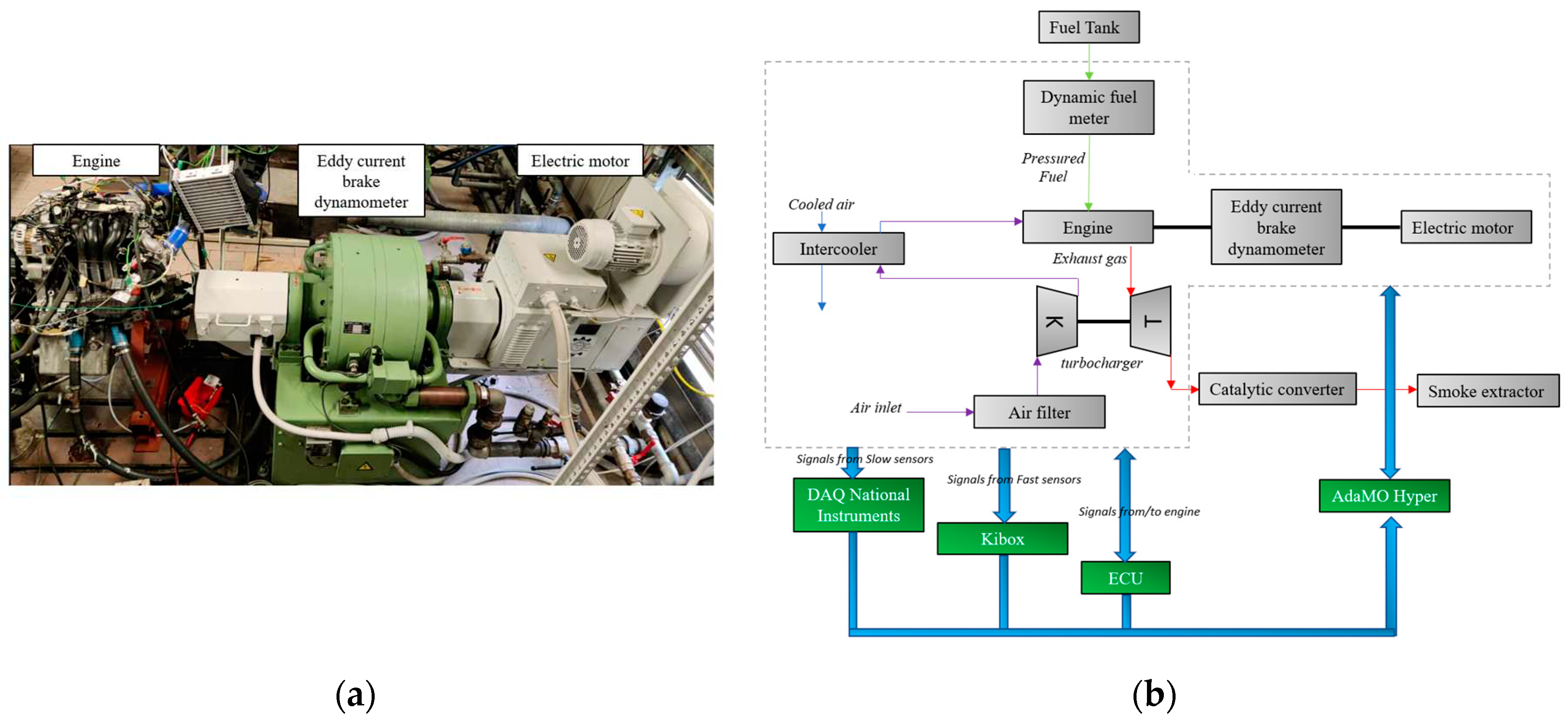
Tests were performed on a 1L 3-cylinder turbocharged engine of 84 CV maximum power at 5250 rpm and 120 Nm of maximum torque at 3250 rpm. The internal cylinder bore is 72 mm while the piston stroke is 81.8 mm. The compression ratio is equal to 10:1. The engine operates in Port Fuel Injection (PFI) with European market gasoline (E5, with RON = 95 and MON= 85) injected at 4.2 bar absolute. A Borghi&Saveri eddy current brake dynamometer of 600 CV ensures the engine speed in firing condition (
Figure 1a). A Vascat electric motor of 66.2 kW allows controlling the engine speed both in motored and firing conditions. All the engine parameters are controlled using an EFI EURO-4 engine control unit. The signals coming from thermocouples TCK and pressure sensors PTX 1000 are acquired by data acquisition systems of National Instrument. The indicated analysis is performed through a Kistler Kibox combustion analysis system (maximum temporal resolution of 0.1 CAD) that acquires the pressure signals coming from the piezoresistive sensors (Kistler 4624A) placed in the intake and exhaust ports, the in-cylinder pressure of the piezoelectric sensor (Kistler 5018) placed on a side of the combustion chamber beside the flywheel, the ignition signal from ECU and the absolute crank angular position measured by an optical encoder (AVL 365C). Due to structural and mechanical constraints, only the combustion chamber adjacent to the flywheel has been equipped with a piezoelectric sensor, which is used to determine the Indicated Mean Effective Pressure (IMEP). The torque delivered by the engine is measured using a torquemeter positioned near the engine crankshaft. All of the above quantities are recorded by AdaMo Hyper software during engine operations, allowing simultaneous management of the engine's speed, torque, and valve throttle position in both firing and motored states.
Figure 1b summarizes the experimental layout.
2.2. Case Study
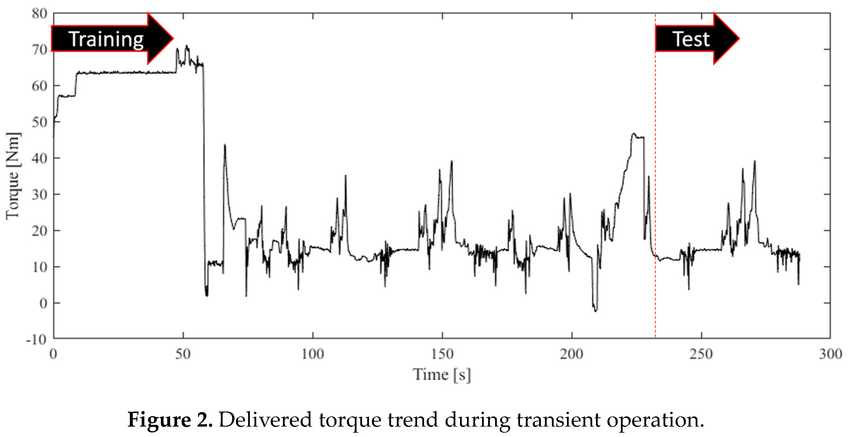
A transient cycle (
Figure 2) has been chosen to preliminarily evaluate the performance of the LSTM+1DCNN proposed algorithm in predicting the torque delivered by the three-cylinder SI engine. A total of 12 variables acquired by AdaMo Hyper are initially selected among the most characteristics, as input parameters.
Parameters coming from ECU: activation time of the injector (InjectionTime) and ignition timing of the spark (SparkAdvance) at the first cylinder beside the flywheel.
Parameters coming from pressure sensors and thermocouples: temperature of the air before the filter (TC_Air_Intake), temperature and pressure of the air at the intake pipe (TC_ETB_OUT and MAP), pressure and temperature of the exhaust gas before (TC_Turbine IN, P_Turbine IN) and after the turbine (TC_Turbine OUT and P_Turbine OUT), temperature of the engine oil (TC_Engine Oil).
Parameters related to the AdaMo actuation: throttle valve opening (Throttle Position) and engine speed (Engine speed).
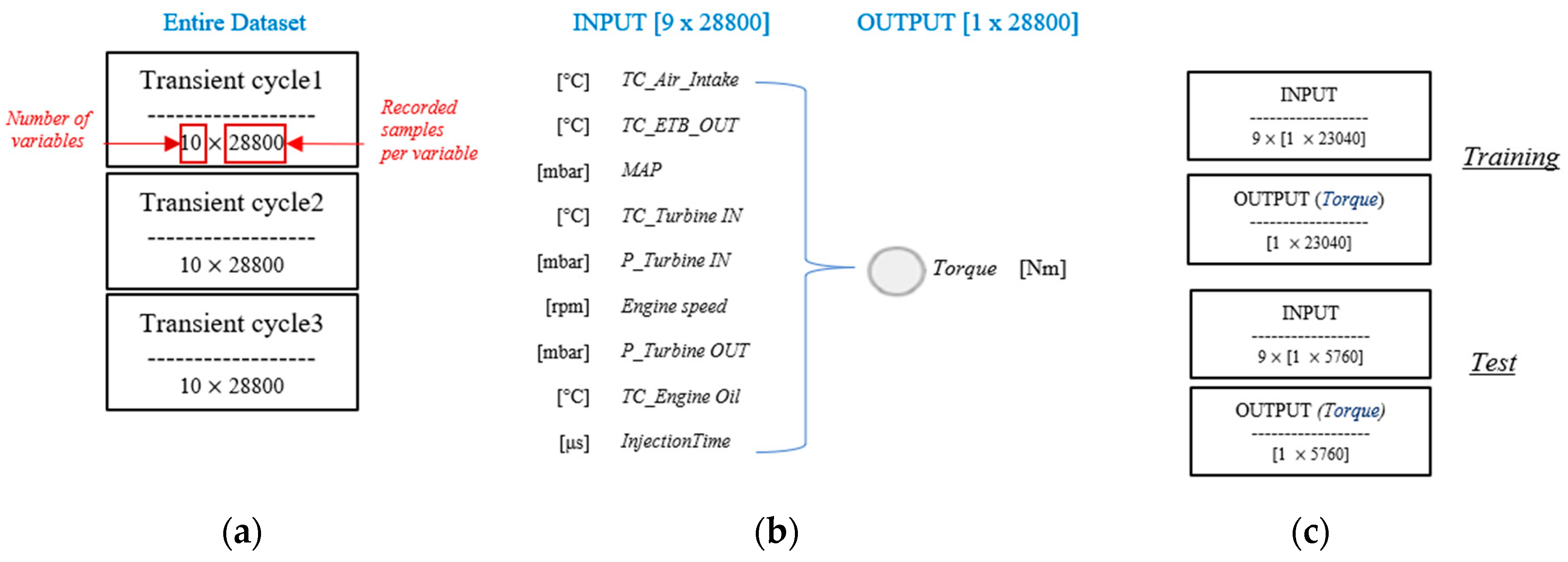
The cycle is comprised of an input matrix of [12 × 28800] samples and of an output matrix of [1 × 28800] samples. 80% of the entire dataset is used for training sessions and the remaining 20% for the test sessions, i.e. Torque prediction (
Figure 2).
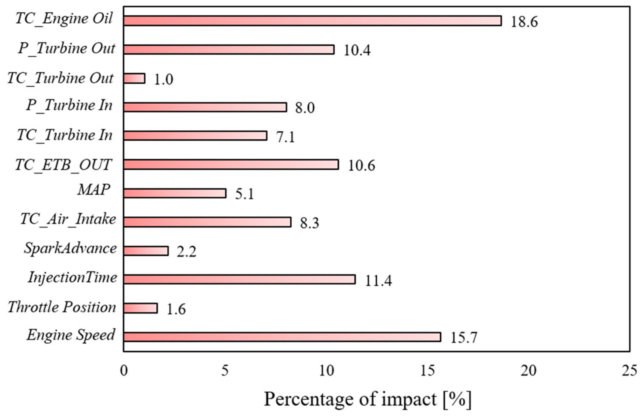
It is feasible to efficiently reduce the dimensions of the model and improve its accuracy by removing parameters with low correlation. As a result, a preliminary analysis using the Shapley value was done on the complete dataset. SHAP attempts to explain an instance's prediction by assessing the contribution of each attribute to the forecast. The authors were able to quantify the impact of the single measured quantities on the objective function using the average absolute Shapley values (ABSV) [
21,
22]. The less influential parameters, i.e. TC_Turbine OUT, SparkAdvance and Throttle Position (
Figure 3) are excluded by the initial input dataset since presenting the lowest percentage of impact. In this way, the number of input parameters is reduced from 12 to 9.
Previous work by the same research group [
2,
20] shown that when the architectures operate with the removal of the less relevant parameters, the performance improves. Based on this, the current work solely illustrates the architectural predicting performance with the previously established 9 input variables. After identifying the input parameters using the prior analysis, the data is normalized to reduce excessive prediction mistakes and to allow the architecture to converge faster. In this context, the normalization process allows for the avoidance of problems caused by differences in input and output parameters. The values supplied are mapped to the range [0, 1]. Following the prediction procedure, the predicted data is de-normalized to provide a direct comparison with the actual experimentally acquired target.
Figure 4 describes the entire dataset used in this activity and the division between input and output parameters for each analyzed case.
2.3. Designing of the Neural Architecture to Predict Engine Torque
2.3.1. Structure of the Proposed Model
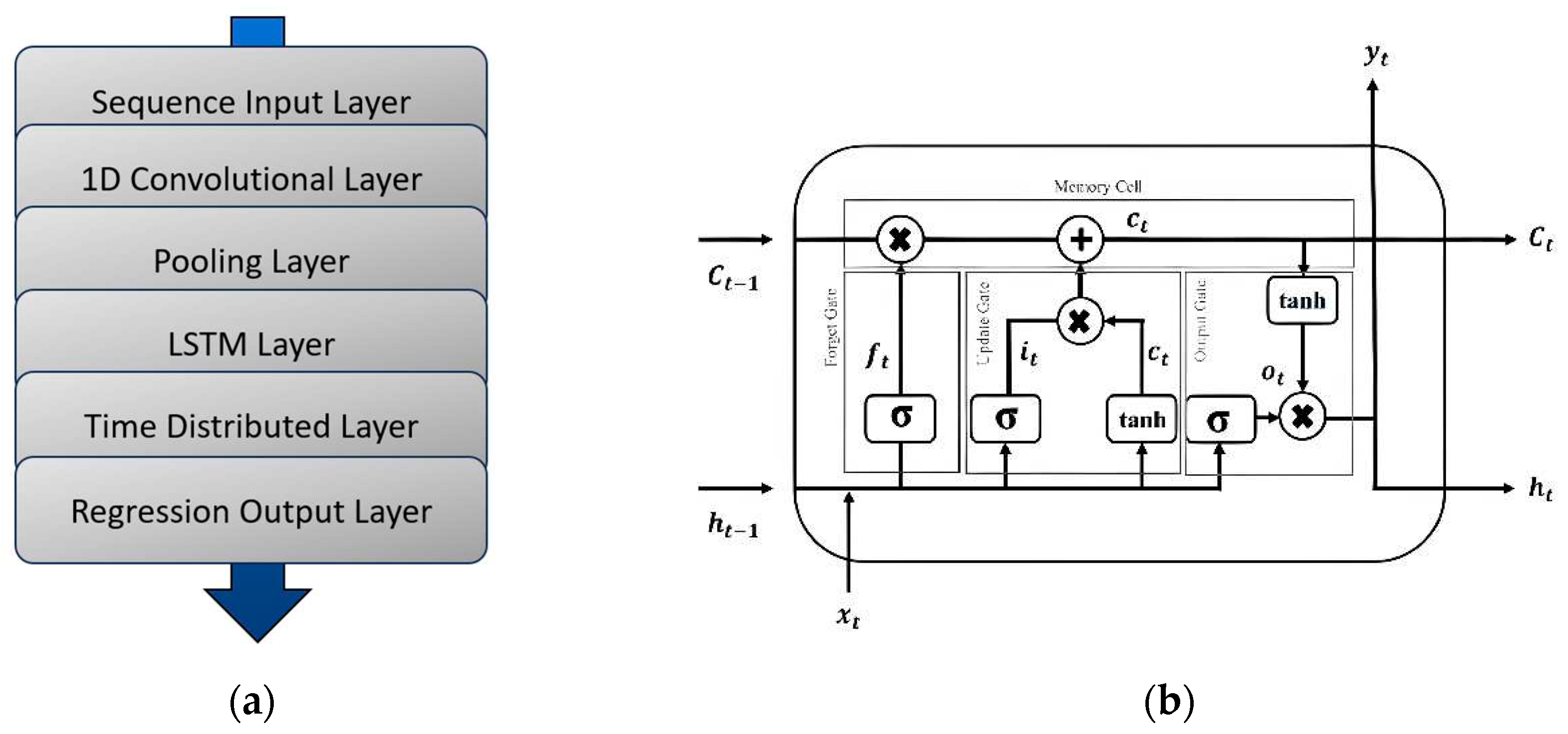
The predictive scheme of the LSTM+1DCNN structure used in this work for the Torque prediction is reported in
Figure 5a.
In the following stage, another 1D convolutional level, similar to the previous one, is used. LSTM is used to process the feature maps at this point. The internal architecture of the LSTM network is made up of components known as gates (
Figure 5b) [
20]. The LSTM network is a sort of recurrent neural network (RNN) that handles the issue of gradients receding or exploding during long-term information propagation. The LSTM network, unlike typical RNNs, has a more sophisticated neuron structure in the hidden layer. It uses three control mechanisms: the input gate, the forgetting gate, and the output gate to retain long-term knowledge. [
26].
LSTMs provide a distinct additive gradient structure with direct access to forget gate activations, allowing the network to encourage desired behavior from the error gradient by employing frequent port updates at each stage of the learning process [
20]. Following LSTM, the feature map is distributed in a temporal vectorial sequence by TimeDistributedLayer, and the loss of mean square error for the specified regression issue is computed by RegressionOutputLevel.
2.3.2. Optimization of the Proposed Model
The definition of the neural structure is determined through preliminary analysis by considering the training sessions’ performance:
The number of neurons in hidden layers Nh varies from 50 to 200.
The batch size Bs is varied from 10 to 100.
The model depth Md is varied from 1 to 10.
A total of 81 combinations are evaluated. The Adam optimizer is used to streamline the updating of the LSTM network model's weight matrix and bias, as well as to adjust the learning rate adaptively during the training process. To evaluate the performance of model parameters, the loss function is created, and the mean square error (MSE) is chosen as the loss function [
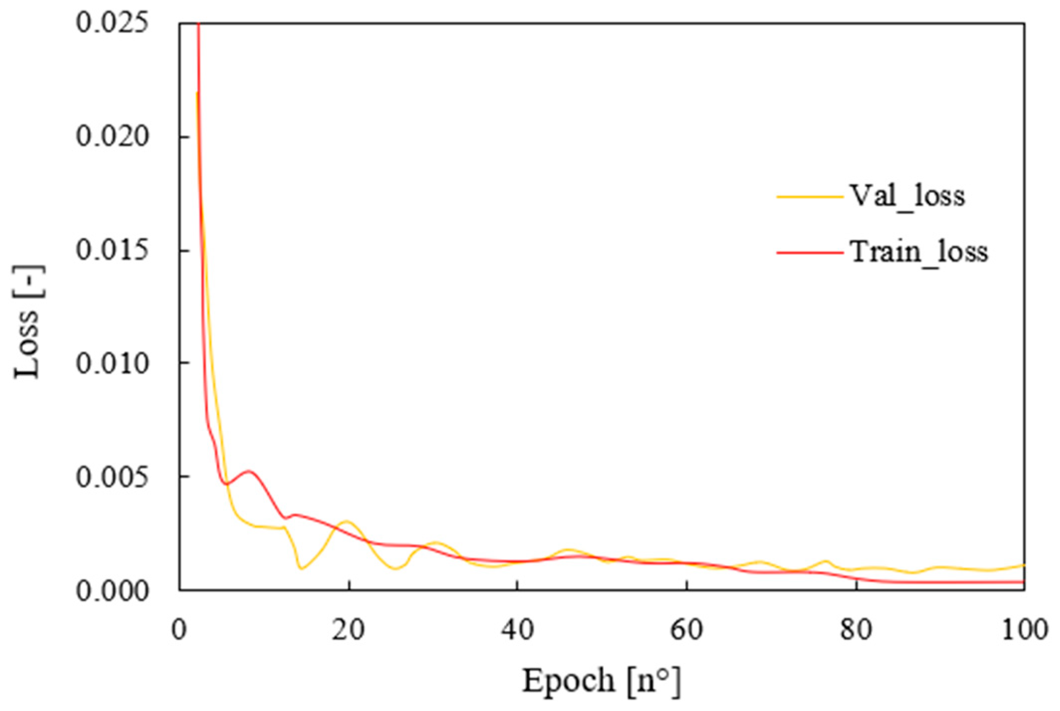
27]. Set the number of network epoch iterations, for example, to 100, to calculate the final value of the loss function for each prediction model once the network training reaches the maximum learning iteration. To predict the Torque signal, the optimal solution with the lowest loss function value is chosen. For the sake of clarity,
Figure 6 shows the val_loss and training_loss of the structure which performed best, i.e., N
h =150, B
s = 70, M
d =1. The training results highlight how the model converges without overfitting.
To sum up, The LSTM+1DCNN structure is composed of a one-dimensional convolutional layer with 100 neurons, kernel size equal to 3, and ReLu activation function; a max pooling 1D layer which uses a pool size of 2 and a stride of 2; a LSTM layer composed by 150 neurons, batch size equal to 70 and model depth is 1; a time distributed layer and a dense layer composed by 1 unit to perform regression task. The performance of the proposed structures is compared with those deriving from the utilization of other two different architectures, whose optimizations have been performed through extensive preliminary analysis:
The structure of a Back Propagation (BP) algorithm [
28] is composed of one input layer, three hidden layers, each of which is comprised of 55,180 and 110 neurons, respectively, and one output layer.
A LSTM [
20] network prediction model composed of one input layer, one hidden layer containing 150 neurons, respectively, one output layer, and one fully connected layer.
3. Results and Discussion
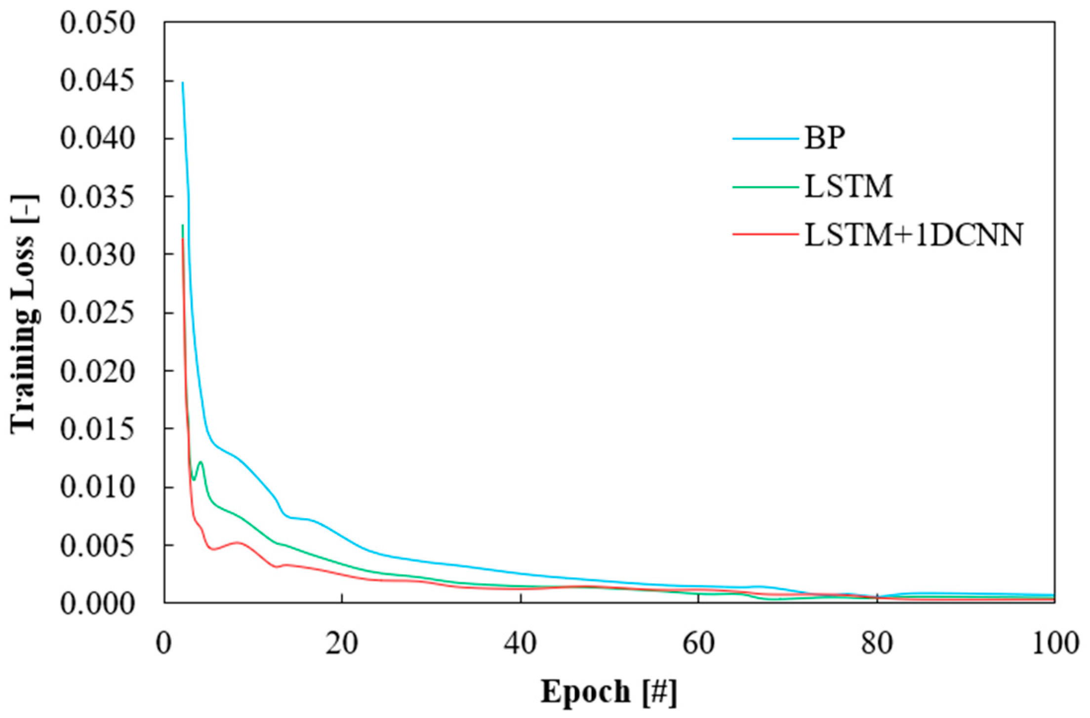
The first comparison between the proposed algorithm is performed via training_loss function (
Figure 7) as described in the previous paragraph. All the structures show a decrease trend as epochs increase and they tend to stabilize around 50 epochs up to reaching a training_loss value lower than 0.001 around the 100
th epoch. This certifies that the models converge without overfitting. In particular, LSTM+1DCNN shows the fastest converge speed since showing training loss below 0.005 already at about 10 epochs. Moreover, once stabilized, it presents very low oscillations suggesting that the model could be more robust than the others.
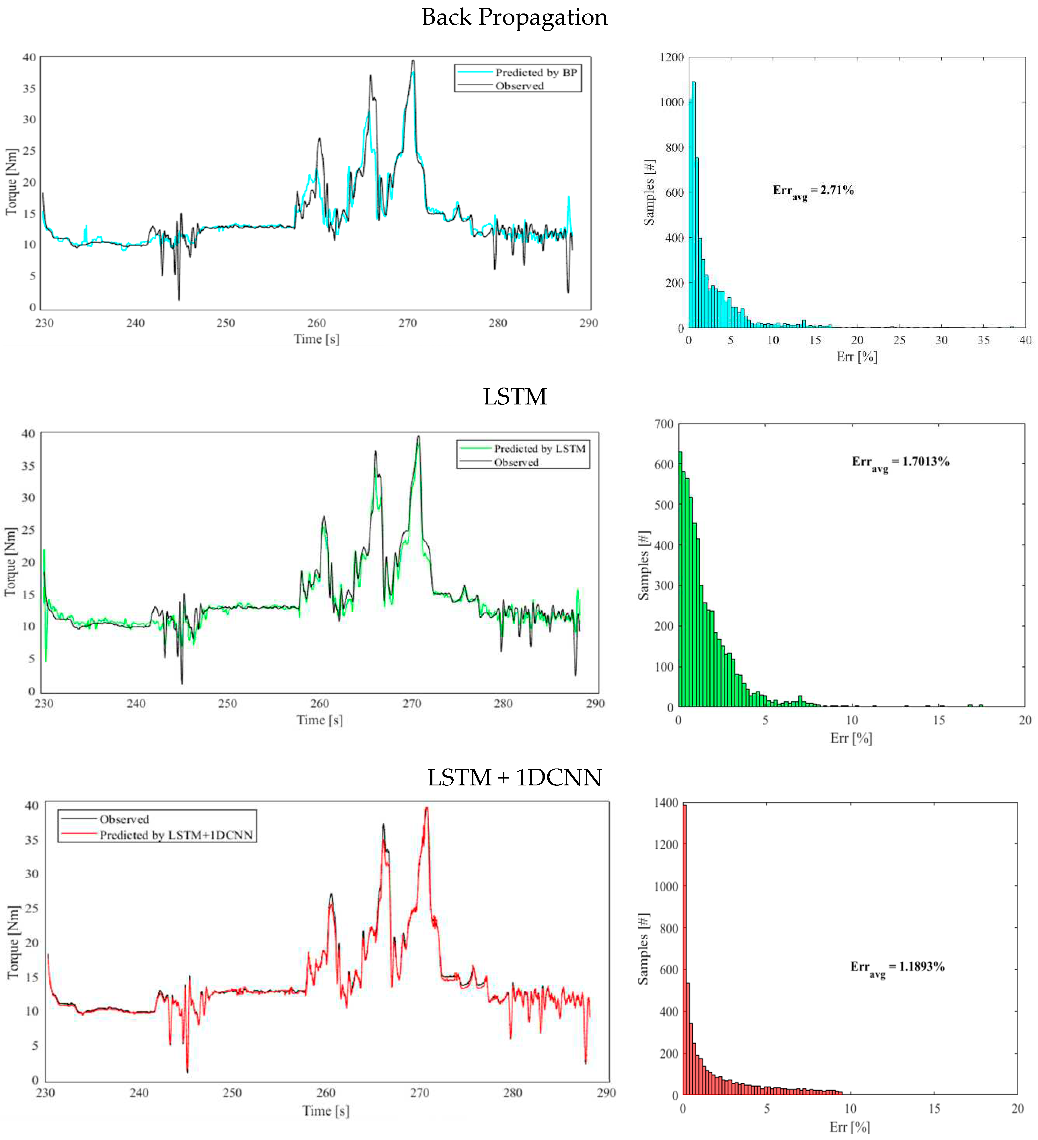
Figure 8 displays the prediction of the Torque traces performed by each tested structure. To make a comparison over the entire predicted range, for each forecast, the average deviation of the prediction from the target throughout the range is computed (1):
where N is the number of samples considered for the test case and i the ith sample. The average percentual error, i.e. Err
avg, is computed as well to draw attention to the global prediction quality. For this kind of application, a maximum critical threshold of 10 is established for the abovementioned errors.
All the tested structures (
Figure 8) are able to reproduce the trend of the Torque over time. Starting from BP, the structure performs an average error of about 2.7%, less than the critical threshold of 10. The number of predictions exceeding such a threshold is 320 samples, corresponding to about 5.55% of the total predictions. The structure is capable of following the low fluctuations of the target signal, while when the torque becomes higher in the range between 250 to 280 seconds, the model underestimates the maximum peaks even if the percentual errors stay below critical thresholds. In such a zone, the architecture predicts in advance the target peaks showing underestimations of about 2 Nm, corresponding to Err higher than 6%. However, it is worth highlighting the structure’s capability of following the fluctuation of the signals in such a large range from 22 to 34 Nm. Concerning LSTM, such a model outperforms the BP performance since presenting Err
avg = 1.70% with 67 samples exceeding Err = 10%, corresponding to 1.16% of the total predictions. With respect to BP, LSTM never exceeds Err by 20%. LSTM is capable of following the low fluctuations of the target and, in the range of highest Torque values, i.e. between 250 to 280 seconds, well-reproduces the peaks without any advances or delays. At around 265 seconds (second highest peak zone) the structure underestimates the target value of about 1.5 Nm. According to the LSTM+1DCNN structure, the architecture is capable of well-reproducing the target trend with average percentage errors below 1.5%, i.e. Err
avg = 1.19%. The prediction never exceeds 10% of error throughout the entire torque signal and better follow the rapid oscillations of the signals if compared to the other architectures.
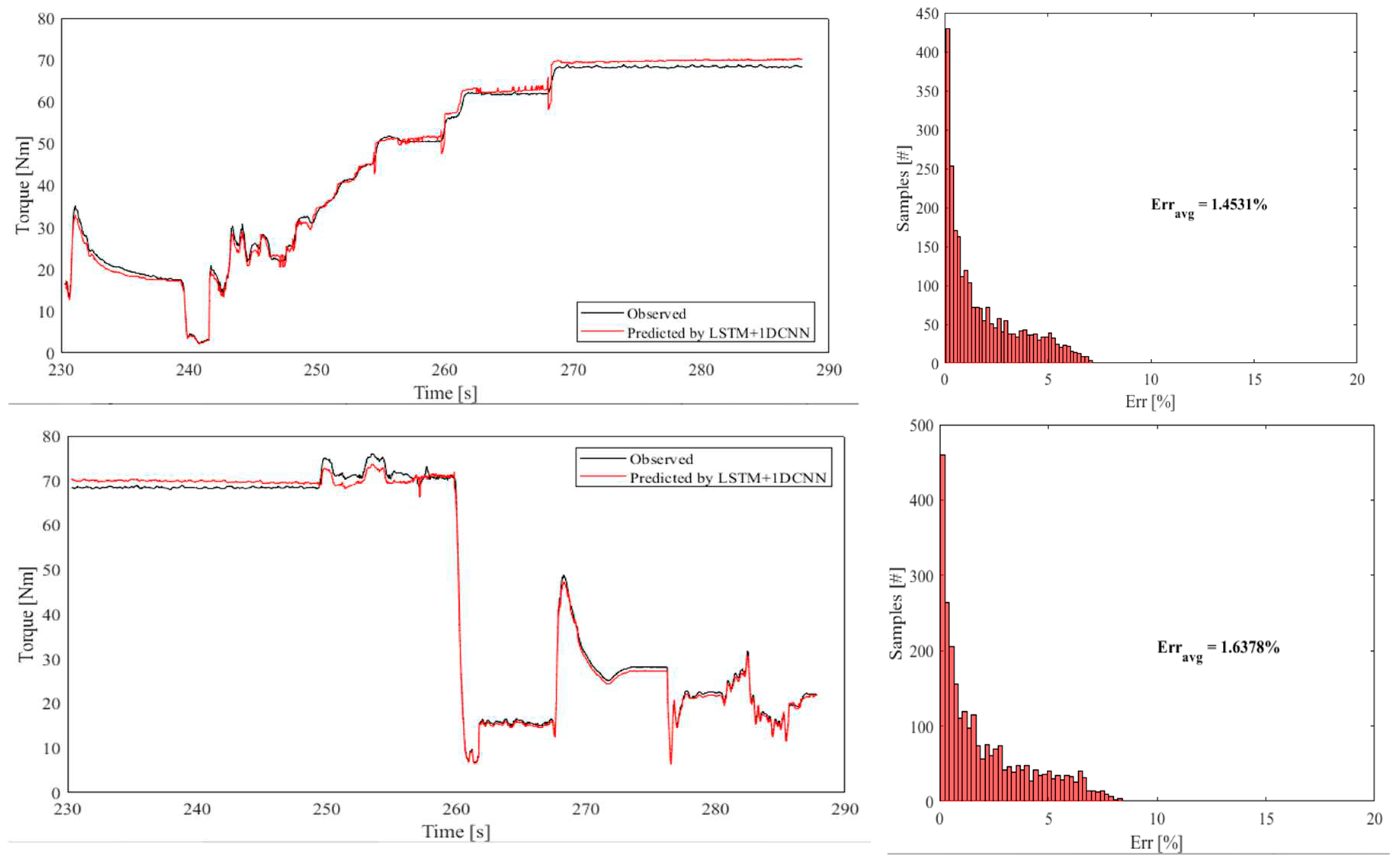
After comparing the prediction performance, and considering the obtained results, the proposed LSTM+1DCNN structure has been tested on another two transient cycles presenting different trends, compared to the case of
Figure 2, but the same number of samples (
Figure 9). As possible to observe, the structure confirms its capability to reproduce the Torque trend, showing average percentual errors below 1.7% and no predictions above 10% of Err, in both reported cases.
4. Conclusions
The present work evaluates the possibility of replacing a physical sensor dedicated to computing the torque delivered by an internal combustion engine, under transient condition, by using a LSTM+1DCNN approach. The optimized structure combines the capability of LSTM to capture long-term dependencies and temporal pattern with the ability of 1DCNN to detect patterns within smaller signal segments. The performance of the proposed architecture was compared with the ones of other optimized artificial neural structures, i.e. Back Propagation and LSTM, used for comparative purposes. All the structures proved to be able to reproduce the experimental trend of the engine delivered torque. Specifically, BP model achieved average error of about 3% with 6% of prediction exceeding the critical threshold set at 10%. It accurately reproduced low fluctuations of the signals but underestimated the maximum peaks of the torque. LSTM overperformed BP showing an average error of 1.7% with about 1.6% of predictions exceeding the critical threshold. Even in this case, underestimations of the local maximum peaks were shown. With average errors of less than 1.5% (Erravg = 1.19%), the LSTM+1DCNN structure outperforms dealing architectures. It follows torque trends properly, never going over a 10% inaccuracy, and captures fast signal oscillations better. The structure's performance was confirmed further in testing on two additional transient cycles, with average errors maintained at 1.7% and no forecasts above 10% inaccuracy. Overall, the study shows that LSTM+1DCNN can replace physical sensors in torque computation for spark-ignition engines.
Author Contributions
Conceptualization, L.P. and F.R.; methodology, F.R.; software, F.R.; validation, L.P., F.R.; formal analysis, L.P. and F.R.; investigation, F.R.; re-sources, F.M.; data curation, F.R.; writing—original draft preparation, F.R.; writing re-view and editing, L.P.; visualization, L.P.; supervision, F.M.; project administration, F.M.; funding acquisition, F.M. All authors have read and agreed to the published version of the manuscript.
Funding
This research received no external funding.
Data Availability Statement
The data presented in this study are available from the corresponding author. The data are not publicly available due to privacy-related choices.
Conflicts of Interest
The authors declare no conflict of interest.
Nomenclature
| Err |
Percentage Errors |
| Erravg
|
Average Percentage Errors |
| ABSV |
Absolute Shapley Values |
| CNN |
Convolutional Neural Network |
| ECU |
Engine Control Unit |
| ICE |
Internal Combustion Engine |
| ML |
Machine Learning |
| LSTM |
Long Short-Term Memory |
| MON |
Motor Octane Number |
| PFI |
Port Fuel Injection |
| RON |
Research Octane Number |
| SI |
Spark Ignition |
References
- Lim, K.Y.H.; Zheng, P.; Chen, C.-H. A state-of-the-art survey of Digital Twin: techniques, engineering product lifecycle management and business innovation perspectives. J. Intell. Manuf. 2019, 31, 1313–1337. [Google Scholar] [CrossRef]
- Ricci, F.; Petrucci, L.; Mariani, F. Using a Machine Learning Approach to Evaluate the NOx Emissions in a Spark-Ignition Optical Engine. Information 2023, 14, 224. [Google Scholar] [CrossRef]
- Reitz, R.D.; Ogawa, H.; Payri, R.; Fansler, T.; Kokjohn, S.; Moriyoshi, Y.; Agarwal, A.; Arcoumanis, D.; Assanis, D.; Bae, C.; et al. IJER editorial: The future of the internal combustion engine. Int. J. Engine Res. 2020, 21, 3–10. [Google Scholar] [CrossRef]
- R. Fiifi, F. R. Fiifi, F. Yan, M. Kamal, A. Ali, and J. Hu, “Engineering Science and Technology, an International Journal Artificial neural network applications in the calibration of spark-ignition engines: An overview,” Eng. Sci. Technol. an Int. J., vol. 19, no. 3, pp. 1346. [Google Scholar]
- Petrucci, L.; Ricci, F.; Mariani, F.; Discepoli, G. A Development of a New Image Analysis Technique for Detecting the Flame Front Evolution in Spark Ignition Engine under Lean Condition. Vehicles 2022, 4, 145–166. [Google Scholar] [CrossRef]
- Petrucci, L.; Ricci, F.; Mariani, F.; Cruccolini, V.; Violi, M. Engine Knock Evaluation Using a Machine Learning Approach. 2020. [CrossRef]
- Srinivasu, P.N.; SivaSai, J.G.; Ijaz, M.F.; Bhoi, A.K.; Kim, W.; Kang, J.J. Classification of skin disease using deep learning neural networks with MobileNet V2 and LSTM. Sensors 2021, 21, 2852. [Google Scholar] [CrossRef] [PubMed]
- Ankobea-Ansah, K.; Hall, C.M. A Hybrid Physics-Based and Stochastic Neural Network Model Structure for Diesel Engine Combustion Events. Vehicles 2022, 4, 259–296. [Google Scholar] [CrossRef]
- Krepelka, M.; Vrany, J. Synthesizing Vehicle Speed-Related Features with Neural Networks. Vehicles 2023, 5, 732–743. [Google Scholar] [CrossRef]
- Fadairo, A.; Ip, W.F. A Study on Performance Evaluation of Biodiesel from Grape Seed Oil and Its Blends for Diesel Vehicles. Vehicles 2021, 3, 790–806. [Google Scholar] [CrossRef]
- A Escobar, C.; Morales-Menendez, R. Machine learning techniques for quality control in high conformance manufacturing environment. Adv. Mech. Eng. 2018, 10. [Google Scholar] [CrossRef]
- Petrucci, L.; Ricci, F.; Martinelli, R.; Mariani, F. Detecting the Flame Front Evolution in Spark-Ignition Engine under Lean Condition Using the Mask R-CNN Approach. Vehicles 2022, 4, 978–995. [Google Scholar] [CrossRef]
- Wang, K.; Ma, C.; Qiao, Y.; Lu, X.; Hao, W.; Dong, S. A hybrid deep learning model with 1DCNN-LSTM-Attention networks for short-term traffic flow prediction. Phys. A: Stat. Mech. its Appl. 2021, 583, 126293. [Google Scholar] [CrossRef]
- Elmaz, F.; Eyckerman, R.; Casteels, W.; Latré, S.; Hellinckx, P. CNN-LSTM architecture for predictive indoor temperature modeling. Build. Environ. 2021, 206, 108327. [Google Scholar] [CrossRef]
- Zhao, J.; Deng, F.; Cai, Y.; Chen, J. Long short-term memory - Fully connected (LSTM-FC) neural network for PM2.5 concentration prediction. Chemosphere 2019, 220, 486–492. [Google Scholar] [CrossRef] [PubMed]
- Wang, X.; Mao, D.; Li, X. Bearing fault diagnosis based on vibro-acoustic data fusion and 1D-CNN network. Measurement 2020, 173, 108518. [Google Scholar] [CrossRef]
- Ren, L.; Dong, J.; Wang, X.; Meng, Z.; Zhao, L.; Deen, M.J. A Data-Driven Auto-CNN-LSTM Prediction Model for Lithium-Ion Battery Remaining Useful Life. IEEE Trans. Ind. Informatics 2020, 17, 3478–3487. [Google Scholar] [CrossRef]
- Qin, Chengjin, et al. "Anti-noise diesel engine misfire diagnosis using a multi-scale CNN-LSTM neural network with denoising module." CAAI Transactions on Intelligence Technology (2023).
- Lyu, Z.; Jia, X.; Yang, Y.; Hu, K.; Zhang, F.; Wang, G. A comprehensive investigation of LSTM-CNN deep learning model for fast detection of combustion instability. Fuel 2021, 303. [Google Scholar] [CrossRef]
- Petrucci, L.; Ricci, F.; Mariani, F.; Mariani, A. From real to virtual sensors, an artificial intelligence approach for the industrial phase of end-of-line quality control of GDI pumps. Measurement 2022, 199. [Google Scholar] [CrossRef]
- Tang, S.; Ghorbani, A.; Yamashita, R.; Rehman, S.; Dunnmon, J.A.; Zou, J.; Rubin, D.L. Data valuation for medical imaging using Shapley value and application to a large-scale chest X-ray dataset. Sci. Rep. 2021, 11, 1–9. [Google Scholar] [CrossRef]
- S. Hart, “Shapley value.” Game Theory, Palgrave Macmillan, London, 1989, pp. 210–216.
- Ozcanli, A.K.; Baysal, M. Islanding detection in microgrid using deep learning based on 1D CNN and CNN-LSTM networks. Sustain. Energy, Grids Networks 2022, 32. [Google Scholar] [CrossRef]
- Bai, Y. RELU-Function and Derived Function Review. SHS Web Conf. 2022, 144, 02006. [Google Scholar] [CrossRef]
- Zafar, A.; Aamir, M.; Nawi, N.M.; Arshad, A.; Riaz, S.; Alruban, A.; Dutta, A.K.; Almotairi, S. A Comparison of Pooling Methods for Convolutional Neural Networks. Appl. Sci. 2022, 12, 8643. [Google Scholar] [CrossRef]
- Hu, H.; Xia, X.; Luo, Y.; Zhang, C.; Nazir, M.S.; Peng, T. Development and application of an evolutionary deep learning framework of LSTM based on improved grasshopper optimization algorithm for short-term load forecasting. J. Build. Eng. 2022, 57. [Google Scholar] [CrossRef]
- Ćalasan, M.; Aleem, S.H.A.; Zobaa, A.F. On the root mean square error (RMSE) calculation for parameter estimation of photovoltaic models: A novel exact analytical solution based on Lambert W function. Energy Convers. Manag. 2020, 210, 112716. [Google Scholar] [CrossRef]
- Cui, Y.; Liu, H.; Wang, Q.; Zheng, Z.; Wang, H.; Yue, Z.; Ming, Z.; Wen, M.; Feng, L.; Yao, M. Investigation on the ignition delay prediction model of multi-component surrogates based on back propagation (BP) neural network. Combust. Flame 2021, 237, 111852. [Google Scholar] [CrossRef]
|
Disclaimer/Publisher’s Note: The statements, opinions and data contained in all publications are solely those of the individual author(s) and contributor(s) and not of MDPI and/or the editor(s). MDPI and/or the editor(s) disclaim responsibility for any injury to people or property resulting from any ideas, methods, instructions or products referred to in the content. |
© 2023 by the authors. Licensee MDPI, Basel, Switzerland. This article is an open access article distributed under the terms and conditions of the Creative Commons Attribution (CC BY) license (http://creativecommons.org/licenses/by/4.0/).
