Atangana-Baleanu fractional dynamics of predictive whooping cough model with optimal control analysis

Preprint

Article

Atangana-Baleanu fractional dynamics of predictive whooping cough model with optimal control analysis

Altmetrics

Downloads

152

Views

Comments

A peer-reviewed article of this preprint also exists.

Azhar Iqbal Kashif Butt^*

This version is not peer-reviewed

Submitted:

01 August 2023

Posted:

03 August 2023

You are already at the latest version

Alerts

Abstract

In this study, we construct a new Atangana-Baleanu fractional model for whooping cough disease to predict future dynamics of the disease, as well as to suggest strategies to eliminate the disease in an optimal way. We prove that the proposed model has a unique solution which is positive and bounded. To measure contagiousness of the disease, we determine the reproduction number R0 and use it to examine the local and global stability at equilibrium points that have symmetry. Through sensitivity analysis, we determine parameters of the model that are most sensitive to R0. The ultimate aim of this research is to analyze different disease prevention approaches in order to find the most suitable one. For this, we include the vaccination and quarantine compartments in the proposed model and formulate an optimal control problem to assess the effect of vaccination and quarantine rates on disease control in three distinct scenarios. Firstly, we study the impact of vaccination strategy and conclude findings with presentation of graphical results. Secondly, we examine the impact of quarantine strategy on whooping cough infection with possible elimination from the society. Lastly, we implement vaccination and quarantine strategies together to visualize their combine effect on infection control. In addition to the study of an optimal control problem, we examine the effect of fractional order on disease dynamics as well as the impact of constant vaccination and quarantine rates on disease transmission and control. We determine that the optimal control strategy with the three controls is more effective in reducing the spread of whooping cough infection. Implementation of Toufik-Atangana type numercial scheme both for the state and adjoint equations is another contribution of this article.

Keywords:

Subject: Computer Science and Mathematics - Mathematical and Computational Biology

1. Introduction

Whooping cough is a highly contagious disease that is caused by a bacterium called Bordetella pertussis. Many outbreaks of the disease have occurred in different parts of the world. The history of the disease dates back to late fifteenth century [1]. However, the first recorded outbreak was witnessed in France in 1578. In 1947, a major whooping cough epidemic occurred in Cape Town that registered 107 deaths [2]. In early 2010, a outbreak occurred in USA, Ireland and Israel. More than 10,000 whooping cough cases were reported in California in 2014 and it was declared as the worst outbreak since 1947. According to a report that published in 2014, there were around 24.1 million cases of whooping cough with 160,700 deaths in younger children around the world [3,8]. According to WHO, there were more than 151,000 pertussis cases worldwide in 2018 [3].

Whooping cough is an extremely infectious disease that has become a serious threat to people of all ages specially dangerous to children younger than 5 years. The disease spreads from one infected person to another susceptible person through the droplets released by sneezing or coughing. The symptoms of whooping cough appear gradually and can stay for few weeks to months. Once a person is caught by infection, the first disease symptoms appear within 7 to 10 days. Early stage common symptoms are minor fever, stuffed or runny nose and cough. At this level, it is not easy to apart it from common cold. After early stage symptoms, the coughing fits start that gradually turns into hacking cough, which is followed by whooping. Sickness, vomiting and difficulty in breathing are the other symptoms of disease. The people who contract infection become infectious up to three weeks. Quarantining such people may help to restrict the spread of disease. The risk of complications and the spread of the virus to others can be reduced with early whooping cough diagnosis and treatment. Whooping cough vaccines also provide the highest level of protection against this highly infectious disease.

Whooping cough is still one of the leading causes of death and illness especially in infants around the world. The disease is on the rise again in many parts of the world, including the USA, Australia and the Great Britain. There is no definite explanation for this rise, but it’s thought to be caused by the vaccine losing its effectiveness, the bacterium becoming more aggressive, and improved diagnostics that have resulted in more cases being diagnosed. It is therefore necessary to develop mathematical models that can be used to forecast dynamics of the whooping cough disease and also to propose strategies for eliminating the disease in the most effective manner. In the existing literature, there are very few mathematical models that have been designed for whooping cough to study its dynamics and to propose effective control strategies. In [4], an effective numerical scheme was presented to simulate second order whooping cough model. In 2018, the authors conducted a study on the cost-effectiveness of maternal vaccination for whooping cough in Australia [5]. Whooping cough model with optimal vaccination control was studied in [6]. A whooping cough model was proposed in [7] to analyze the disease transmission in Nebraska. An implicit numerical integration method was established in [8] to ensure a consistent dynamic convergence of the SEIR model for the whooping cough epidemic. In [9], ABC fractional derivative is employed to model phytoplankton nutrient and whooping cough epidemics. The authors, in this article, used homotopy perturbation Elzaki transform method for numerical solutions and proved that the implemented method is an effective technique to handle such fractional models. In all of the above articles, no one has used fractional modeling for whooping cough with optimal control analysis.

Mathematical modeling is a powerful tool for predicting the dynamics of communicable disease with prevention measures. The differential equations for the epidemiological compartmental models have symmetry in the sense that these are constructed on the principle that the rate of change of individuals in a particular compartment is equal to the incoming individuals minus the outgoing individuals. In recent years, many scientists have begun to use fractional models with different fractional operators to include memory effects for better epidemiological disease analysis [10,11,12,13,14,15,16,17,18]. Fractional operators have a wide range of uses in modern mathematics, including the complex and significant study of symmetric systems. Furthermore, fractional models work better and are more consistent with the real data. In this study, we develop a new Atangana-Baleanu-Caputo (ABC) fractional whooping cough model, SVEIQR, with an aim to evaluate the effectiveness of different disease control strategies, including vaccination of susceptible and the isolation of infected individuals, and to observe the influence of fractional order on disease dynamics. The reason of choosing ABC operator for the proposed model is due to its non-local and non-singular kernel. In addition to this, the operator has the ability to capture higher susceptibilities and less infections as compared to other fractional operators, such as Caputo and Caputo-Fabrizo [19]. First of all, we will examine validity of the proposed model by proving basic properties of the model, such as existence of positive and bounded unique solution, local and global stability analysis at equilibrium points. In addition, this article contributes to the development of a fractional optimal control problem to identify optimal vaccination and quarantine rates that will help to limit the spread of whooping cough infection. Symmetry analysis is a robust tool to come up with numerical solutions for a certain fractional differential equations. In this study, we implement Toufik-Atangana type numerical scheme for numerical simulations of state and adjoint equations.

The other sections are organized as follows: In Section 2, we describe the formulation of a

S V E I Q R

fractional model to express dynamics of whooping cough disease. The formulation is given with the help of the Atangana-Baleanu fractional derivative. Theoretical aspects of the proposed fractional model are discussed in Section 3, including the existence and uniqueness of the solution, the positivity and boundedness of the solutions, the calculation of equilibrium points and the determination of fundamental reproduction number

R_{0}

, the analysis of local and global stability at equilibrium points. In Section 4, Toufik-Atangana type numerical scheme is established and implemented to observe the impact of fractional order on disease dynamics. The effect of vaccination and quarantine rates on disease transmission is also simulated here. In Section 5, we provide sensitivity analysis to identify extremely sensitive parameters for reproduction number

R_{0}

. In Section 6, the model is further modified with time dependent controls to form an optimal control problem. The associated optimality conditions arising from Pontryagin’s principle are then numerically solved by applying the Toufik-Atangana numerical scheme for determining the best time-dependent vaccination and quarantine rates for whooping cough control. The results of this study are concluded in Section 7.

2. Model formulation

Mathematical models of infectious diseases play a vital role in understanding disease flow patterns and in designing appropriate disease control strategies. Therefore, while developing a mathematical models for infectious diseases, it is very important to focus on procedures needed in formulating the epidemiology of the disease and to identify the most important and controllable parameters disease control. A variety of epidemiological models have been developed on the basis of disease transmission mechanism and are available in literature, see [20,21,22,23,24,25,26,27]. These models have played a significant role in formulating and designing control strategies for different diseases.

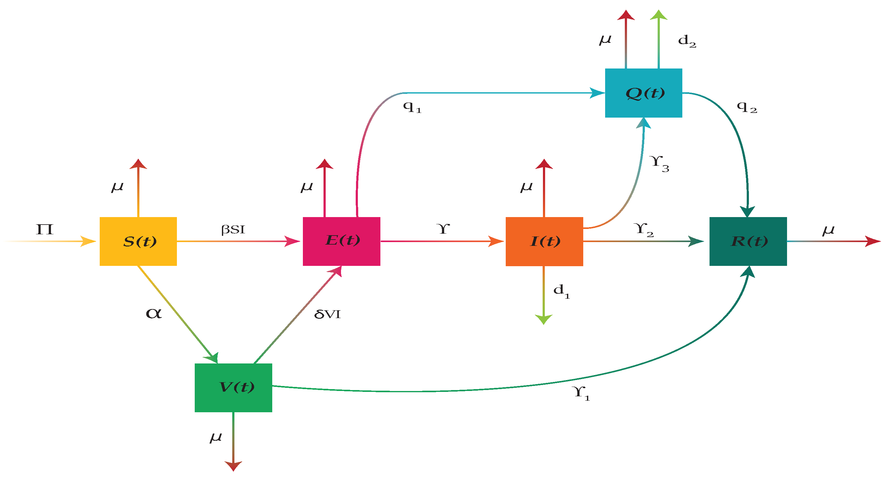
In this study, we develop a new SVEIQR model for whooping cough infectious disease. The aim is to study the disease dynamics comprehensively and to formulate the most suitable control strategies to restrict spread of the disease. We divide the total human population

N (t)

into six compartments: susceptible

S (t)

, vaccinated

V (t)

, exposed

E (t)

, infected

I (t)

, quarantined

Q (t)

and recovered

R (t)

. The humans specified by

S (t)

are those who are at the risk of getting virus after having contact with an infectious person. Thus, the susceptible who caught by virus move to exposed class

E (t)

and those who are vaccinated at the rate

α

move to

V (t)

. The vaccinated individuals may either move to recovered class

R (t)

at the rate

γ_{1}

or to exposed class

E (t)

after getting infection as a result of having contact with an infectious person. The exposed individuals who become infectious move to infected class

I (t)

at the rate

γ

. To restrict the spread of disease, we introduce an isolation compartment

Q (t)

in the model. The individuals from exposed and infected classes are transferred to quarantined class

Q (t)

at rates

q_{1}

and

γ_{3}

respectively. The individuals of

I (t)

and

Q (t)

classes who recovered either by medication or by their natural immunity move to recovered class

R (t)

respectively at the rates

γ_{2}

and

q_{2}

. The rates at which infected and quarantined die due to disease are

d_{1}

and

d_{2}

. Thus, the whole human population at any time t is given by

N (t) = S (t) + V (t) + E (t) + I (t) + Q (t) + R (t) .

(1)

The whooping cough disease flow pattern given in Figure 1 is governed by a mathematical model consisting of the following nonlinear system of coupled ordinary differential equations:

\begin{matrix} \frac{d S}{d t} = & Π - β I S - (μ + α) S, \end{matrix}

(2a)

\begin{matrix} \frac{d V}{d t} = & α S - δ I V - (γ_{1} + μ) V, \end{matrix}

(2b)

\begin{matrix} \frac{d E}{d t} = & β I S + δ I V - (μ + γ + q_{1}) E, \end{matrix}

(2c)

\begin{matrix} \frac{d I}{d t} = & γ E - (γ_{2} + γ_{3} + μ + d_{1}) I, \end{matrix}

(2d)

\begin{matrix} \frac{d Q}{d t} = & q_{1} E + γ_{3} I - (q_{2} + d_{2} + μ) Q, \end{matrix}

(2e)

\begin{matrix} \frac{d R}{d t} = & γ_{1} V + γ_{2} I + q_{2} Q - μ R, \end{matrix}

(2f)

subject to the conditions:

\begin{matrix} S (0) = S_{0} > 0, V (0) = V_{0} \geq 0, E (0) = E_{0} \geq 0, I (0) = I_{0} \geq 0, Q (0) = Q_{0} \geq 0, R (0) = R_{0} \geq 0 . \end{matrix}

(2g)

2.1. Fractional model

Generally, classical integer order models are neither robust nor more useful for understanding the dynamic behavior of an infectious disease. On the other hand, fractional order models work more appropriately with the real data. Hence, to generalize the system (2) for whooping cough, we use fractional Atangana-Baleanu derivative

_{a}^{A B C} D_{t}^{ρ}

, defined in (3), in place of the classical integer order time derivative

D_{t}

. This fractional order formulation will allow us to observe memory impacts and gain further insight into disease dynamics. For the fractional formulation, we first consider some basics related to Atangana-Baleanu fractional derivatives [28].

Definition 1.

[28] If the differentiable function

Φ : [a, b] \to N

is defined on

[a, b]

such that

Φ \in H^{1} (a, b)

b > a

and

σ \in (0, 1]

, then the Atangana-Baleanu derivative of Φ in Caputo sense is defined as:

\begin{matrix} _{a}^{A B C} D_{t}^{σ} Φ (t) = \frac{F (σ)}{1 - σ} \int_{a}^{t} \dot{Φ} (ξ) E_{σ} [- σ \frac{{(t - ξ)}^{σ}}{1 - σ}] d ξ, \end{matrix}

(3)

where

E_{σ}

is a well-known one parameter Mittag-Leffler function and

F (σ)

is a normalizing function such that

F (0) = 1, F (1) = 1

Definition 2.

[28,29] An ABC fractional integral with non-local kernal is defined by

\begin{matrix} _{a}^{A B C} I_{t}^{σ} Φ (t) = \frac{1 - σ}{F (σ)} Φ (t) + \frac{σ}{F (σ) Γ (σ)} \int_{a}^{t} Φ (ξ) {(t - ξ)}^{σ - 1} d ξ . \end{matrix}

(4)

For

t \geq 0

and

σ \in (0, 1]

, the proposed nonlinear fractional order model for whooping cough in the sense of ABC-fractional operator is given as:

\begin{matrix} _{0}^{A B C} D_{t}^{σ} S (t) & = Π - β I S - (μ + α) S, \end{matrix}

(5a)

\begin{matrix} _{0}^{A B C} D_{t}^{σ} V (t) & = α S - δ I V - (γ_{1} + μ) V, \end{matrix}

(5b)

\begin{matrix} _{0}^{A B C} D_{t}^{σ} E (t) & = β I S + δ I V - (μ + γ + q_{1}) E, \end{matrix}

(5c)

\begin{matrix} _{0}^{A B C} D_{t}^{σ} I (t) & = γ E - (γ_{2} + γ_{3} + μ + d_{1}) I, \end{matrix}

(5d)

\begin{matrix} _{0}^{A B C} D_{t}^{σ} Q (t) & = q_{1} E + γ_{3} I - (q_{2} + d_{2} + μ) Q, \end{matrix}

(5e)

\begin{matrix} _{0}^{A B C} D_{t}^{σ} R (t) & = γ_{1} V + γ_{2} I + q_{2} Q - μ R, \end{matrix}

(5f)

with conditions:

\begin{matrix} \begin{matrix} S (0) = S_{0} > 0, V (0) = V_{0} \geq 0, E (0) = E_{0} \geq 0, \\ I (0) = I_{0} \geq 0, Q (0) = Q_{0} \geq 0, R (0) = R_{0} \geq 0 . \end{matrix} \end{matrix}

(5g)

The system (5) is an autonomous, hence it can be written in the following compact form:

\begin{matrix} _{0}^{A B C} D_{t}^{σ} V (t) = G (V (t)), 0 < t < t_{f} < + \infty \end{matrix}

(6a)

along with

\begin{matrix} V (0) = V_{0}, \end{matrix}

(6b)

where

V : [0, + \infty) \to R^{6}

and

G : R^{6} \to R^{6}

are vector valued functions given as:

\begin{matrix} V (t) = (\begin{matrix} S (t) \\ V (t) \\ E (t) \\ I (t) \\ Q (t) \\ R (t) \end{matrix}), V_{0} = (\begin{matrix} S_{0} \\ V_{0} \\ E_{0} \\ I_{0} \\ Q_{0} \\ R_{0} \end{matrix}), G (V (t)) = (\begin{matrix} Π - β I S - (μ + α) S \\ α S - δ I V - (γ_{1} + μ) V \\ β I S + δ I V - (μ + γ + q_{1}) E \\ γ E - (γ_{2} + γ_{3} + μ + d_{1}) I \\ q_{1} E + γ_{3} I - (q_{2} + d_{2} + μ) Q \\ γ_{1} V + γ_{2} I + q_{2} Q - μ R \end{matrix}) . \end{matrix}

3. Theoretical analysis of the proposed model

This section is devoted for a comprehensive theoretical analysis of the proposed fractional model (6) where we investigate some key characteristics of the model and show that the model is well-posed for numerical approximations.

3.1. Existence and uniqueness of solution

First of all, we prove that the solution of model (6) exists and is unique. We make use of some basic definitions and theorems stated in [30] to prove the existence and uniqueness of solution of the proposed fractional model.

Theorem 1.

[30] Every contractive sequence is a Cauchy sequence, and therefore convergent in complete metric space.

Theorem 2.

[31] Let

B \subseteq R

and

Ψ : B \to R^{n}

be a continuously differentiable mapping,

s \in B

. Then, Ψ satisfies a Lipschitz condition on each convex compact subset

B

of B with Lipchitz constant L. Where

L > 0

is the supremum of the derivative of Ψ on

B

, i.e.,

L = sup_{s \in B} ∣ \frac{d Ψ}{d s} ∣

Theorem 3.

The function

G (V)

in equation (6) is Lipschitz continuous.

Proof.

Let

S

be a convex compact subset of

\begin{matrix} S = {(t, V) | 0 \leq t \leq t_{f}, V \in R_{+}^{6}} . \end{matrix}

Let

V_{1}, V_{2} \in S

, then by mean value theorem ∃

ζ \in (V_{1}, V_{2})

such that

\begin{matrix} \frac{G (V_{1} (t)) - G (V_{2} (t))}{V_{1} (t) - V_{2} (t)} = & G^{^{'}} (ζ (t)), \end{matrix}

\begin{matrix} G (V_{1} (t)) - G (V_{2} (t)) = & G^{'} (ζ (t)) . (V_{1} (t) - V_{2} (t)), \end{matrix}

\begin{matrix} ∣ G (V_{1} (t)) - G (V_{2} (t)) ∣ & = ∣ G^{'} (ζ (t)) . (V_{1} (t) - V_{2} (t)) ∣, \\ \leq ∥ G^{'} {(ζ) ∥}_{\infty} {∥ V_{1} - V_{2} ∥}_{\infty} . \end{matrix}

Since

G \in C^{1} [0, t_{f}]

, hence over convex compact set

S

, ∃ a constant

τ > 0

such that

\begin{matrix} ∥ G^{'} {(ζ) ∥}_{\infty} \leq τ, \end{matrix}

hence,

\begin{matrix} ∣ G (V_{1} (t)) - G (V_{2}) (t) ∣ & \leq τ ∥ V_{1} - V_{2} ∥_{\infty} \\ sup_{t \in [0, t_{f}]} ∣ G (V_{1}) - G (V_{2}) ∣ & \leq τ ∥ V_{1} - V_{2} ∥_{\infty} \\ ∥ G (V_{1}) - G (V_{2}) ∥_{\infty} & \leq τ ∥ V_{1} - V_{2} ∥_{\infty} \end{matrix}

Thus,

G (V)

is Lipschitz. □

Theorem 4.

Suppose that the function

G (V)

satisfies the Lipschitz condition

\begin{matrix} ∥ G (V_{2}) - G (V_{1}) ∥_{\infty} \leq τ {∥ V_{2} - V_{1} ∥}_{\infty}, \end{matrix}

then the problem (6) has a unique solution for

\begin{matrix} τ (\frac{1 - σ}{F (σ)} + \frac{σ}{F (σ) Γ (σ)} T^{*}) < 1 . \end{matrix}

Proof.

We shall prove that the function

V (t)

satisfies equation (6) if and only if it satisfies the relation

\begin{matrix} V (t) = V (0) + \frac{1 - σ}{F (σ)} G (V (t)) + \frac{σ}{F (σ) Γ (σ)} \int_{0}^{t} {(t - ξ)}^{σ - 1} G (V (ξ)) d ξ . \end{matrix}

Let

V (t)

satisfies equation (6). We apply Atangana-Beleanu fractional integral (4) to both sides of (6) to get

\begin{matrix} _{0}^{A B C} I_{t}^{σ} [_{0}^{A B C} D_{t}^{σ} V (t)] =_{0}^{A B C} I_{t}^{σ} G (V (t)) . \end{matrix}

Simplification yields us the integral equation:

\begin{matrix} V (t) = V_{0} + \frac{1 - σ}{F (σ)} G (V (t)) + \frac{σ}{F (σ) Γ (σ)} \int_{0}^{t} {(t - ξ)}^{σ - 1} G (V (ξ)) d ξ . \end{matrix}

(7)

Now for converse, we suppose that

V_{n}

is a sequence of solutions that converges to the solution (7) with Picard successive iteration, i.e.

\begin{matrix} V_{n} (t) = V_{0} (t) + \frac{1 - σ}{F (σ)} G (V_{n} (t)) + \frac{σ}{F (σ) Γ (σ)} \int_{0}^{t} {(t - ξ)}^{σ - 1} G (V_{n} (ξ)) d ξ, V_{0} (t) = V_{0} . \end{matrix}

(8)

First of all we show that the sequence (8) is contractive if

τ (\frac{1 - σ}{F (σ)} + \frac{σ}{F (σ) Γ (σ)} T^{*}) < 1,

where

T^{*} = t_{f} Υ

and

Υ = {sup}_{t \in [0, t_{f}]} {(t - ξ)}^{σ - 1}

Consider

\begin{matrix} ∣ V_{n} (t) - V_{n - 1} (t) ∣ = & ∣ \frac{1 - σ}{F (σ)} [G (V_{n - 1} (t)) - G (V_{n - 2} (t))] \\ + \frac{σ}{F (σ) Γ (σ)} \int_{0}^{t} {(t - ξ)}^{σ - 1} [G (V_{n - 1} (x)) - G (V_{n - 2} (x))] d ξ ∣, \\ \leq \frac{1 - σ}{F (σ)} ∣ G (V_{n - 1} (t)) - G (V_{n - 2} (t)) ∣ \\ + \frac{σ}{F (σ) Γ (σ)} \int_{0}^{t} ∣ {(t - ξ)}^{σ - 1} ∣ ∣ G (V_{n - 1} (x)) - G (V_{n - 2}) ∣ d x . \end{matrix}

Using Lipchitz property of function

G (v)

, we get the following expression:

\begin{matrix} ∣ V_{n} (t) - V_{n - 1} (t) ∣ & \leq \frac{1 - σ}{F (σ)} τ ∣ V_{n - 1} (t) - V_{n - 2} (t) ∣ \\ + \frac{σ}{F (σ) Γ (σ)} \int_{0}^{t} ∣ {(t - ξ)}^{σ - 1} ∣ τ ∣ V_{n - 1} (t) - V_{n - 2} (t) ∣ d x, \\ \leq \frac{1 - σ}{F (σ)} α sup_{t \in [0, t_{f}]} ∣ V_{n - 1} (t) - V_{n - 2} (t) ∣ \\ + \frac{σ}{F (σ) Γ (σ)} \int_{0}^{t} τ sup_{t \in [0, t_{f}]} ∣ {(t - ξ)}^{σ - 1} ∣ sup_{t \in [0, t_{f}]} ∣ V_{n - 1} (t) - V_{n - 2} (t) ∣ d x, \\ ∣ V_{n} (t) - V_{n - 1} (t) ∣ & \leq τ (\frac{1 - σ}{F (σ)} + \frac{σ}{F (σ) Γ (σ)} T^{*}) {∥ V_{n - 1} - V_{n - 2} ∥}_{\infty}, \\ sup_{t \in [0, t_{f}]} ∣ V_{n} (t) - V_{n - 1} (t) ∣ & \leq τ (\frac{1 - σ}{F (σ)} + \frac{σ}{F (σ) Γ (σ)} T^{*}) {∥ V_{n - 1} - V_{n - 2} ∥}_{\infty}, \\ ∥ V_{n} - V_{n - 1} ∥_{\infty} & \leq κ ∥ V_{n - 1} - V_{n - 2} ∥_{\infty}, \end{matrix}

where

κ = τ (\frac{1 - σ}{F (σ)} + \frac{σ}{F (σ) Γ (σ)} T^{*}) < 1 .

This implies that

d (V_{n}, V_{n - 1}) \leq κ d (V_{n - 1}, V_{n - 2}) .

(9)

Thus from equation (9), sequence (8) is contractive, hence Theorem 1 implies it is a Cauchy sequence. Now for

p, q \in N

and

p > q

\begin{matrix} ∣ V_{p} - V_{q} ∣ = & ∣ V_{p} - V_{p - 1} + V_{p - 1} - V_{p - 2} + V_{p - 2} . . . - V_{q + 1} + V_{q + 1} - V_{q} ∣, \\ \leq ∣ V_{p} - V_{p - 1} ∣ + ∣ V_{p - 1} - V_{p - 2} ∣ + . . . + ∣ V_{q + 1} - V_{q} ∣, \\ \leq κ^{p - 1} ∣ V_{1} - V_{0} ∣ + κ^{p - 2} ∣ V_{1} - V_{0} ∣ + . . . + κ^{q} ∣ V_{1} - V_{0} ∣, \\ \leq [κ^{p - 1} + κ^{p - 2} + . . . + κ^{q}] ∣ V_{1} - V_{0} ∣ . \end{matrix}

Right hand side is a geometric series which is always convergent for

0 < κ < 1

\begin{matrix} ∣ V_{p} - V_{q} ∣ \leq & κ^{q} \frac{1 - κ^{p - q}}{1 - κ} ∣ V_{1} - V_{0} ∣ \leq κ^{q} \frac{1}{1 - κ} ∣ V_{1} - V_{0} ∣ \end{matrix}

Since

0 < κ < 1

l i m (κ^{q}) = 0

. Therefore, we infer that sequence

(V_{n})

is Cauchy and hence by a theorem from [30] it is convergent. Let

l i m (V_{n}) = V

, then equation (8) gives

\begin{matrix} l i m_{n \to \infty} V_{n} (t) = V (t) = v (0) + \frac{1 - σ}{F (σ)} G (V (t)) + \frac{σ}{F (σ) Γ (σ)} \int_{0}^{t} {(t - ξ)}^{σ - 1} G (v (ξ)) d ξ, \end{matrix}

(10)

which is the required solution.

Uniqueness For uniqueness of the solution, we assume on contrary that the sequence

(V_{n})

converges to two limits

V_{1}

and

V_{2}

such that

V_{1} \neq V_{2}

. Then, there exist

n_{1} a n d n_{2} \in N

such that,

\begin{matrix} ∣ V_{n} - V_{1} ∣ < ϵ_{1}, n_{1} \geq n . \\ ∣ V_{n} - V_{2} ∣ < ϵ_{2}, n_{2} \geq n . \end{matrix}

Let

n = m a x {n_{1}, n_{2}}

. Then,

\begin{matrix} ∣ V_{1} - V_{2} ∣ = ∣ V_{1} - V_{n} + V_{n} - V_{2} ∣ \leq ∣ V_{1} - V_{n} ∣ + ∣ V_{n} - V_{2} ∣ < ϵ_{1} + ϵ_{2} = ϵ, \end{matrix}

which implies,

\begin{matrix} ∣ V_{1} - V_{2} ∣ = 0 \Rightarrow V_{1} = V_{2} . \end{matrix}

Hence, it is proved that the solution (10) is a unique solution of (6) or equivalently of the system (5). □

3.2. Boundedness and positivity of the solutions

Next, we prove another property of the model, i.e. we prove that the model (5) has a positive and bounded solution for

t \geq 0

Theorem 5.

The solution

y (t) = (S (t), V (t), E (t), I (t), Q (t), R (t))

of the model (5) is bounded.

Proof.

Applying Atangana-Baleanu-Caputo derivative operator

_{0}^{A B C} D_{t}^{σ}

to (1), we have

\begin{matrix} _{0}^{A B C} D_{t}^{σ} N (t) = & _{0}^{A B C} D_{t}^{σ} S (t) +_{0}^{A B C} D_{t}^{σ} V (t) +_{0}^{A B C} D_{t}^{σ} E (t) +_{0}^{A B C} D_{t}^{σ} I (t) \\ +_{0}^{A B C} D_{t}^{σ} Q (t) +_{0}^{A B C} D_{t}^{σ} R (t), \\ = & Π - d_{1} I - d_{2} Q - μ N . \end{matrix}

Since

d_{1} I + d_{2} Q \geq 0

, so

\begin{matrix} _{0}^{A B C} D_{t}^{σ} N (t) \leq Π - μ N (t) . \end{matrix}

We apply Laplace transform on both sides of the above inequality to obtain:

\begin{matrix} L {_{0}^{A B C} D_{t}^{σ} N (t)} (s) \leq \frac{Π}{s} - μ L {N (t)} (s), \end{matrix}

and

\begin{matrix} \frac{F (σ) s^{σ}}{σ + (1 - σ) s^{σ}} N (s) + μ N (s) \leq Π s^{- 1} + \frac{F (σ) N (0) s^{σ - 1}}{σ + (1 - σ) s^{σ}}, \end{matrix}

(11)

where

N (0)

represents the initial value of the total population.

Inequality (11) is solved to get:

\begin{matrix} N (s) \leq \frac{Π Ω}{μ} \frac{s^{σ - (σ + 1)}}{s^{σ} + Ω} + \frac{Ω}{μ σ} [Π (1 - σ) + F (σ) N (0)] \frac{s^{σ - 1}}{s^{σ} + Ω}, \end{matrix}

(12)

where

Ω = \frac{σ μ}{F (σ) + (1 - σ) μ}

Application of inverse Laplace transform on both sides of (12) gives us:

\begin{matrix} N (t) \leq \frac{Π Ω}{μ} E_{σ, σ + 1} (- Ω t^{σ}) + \frac{Ω}{μ σ} [Π (1 - σ) + F (σ) N (0)] E_{σ, 1} (- Ω t^{σ}) . \end{matrix}

(13)

Since the Mittag-Leffler function

\begin{matrix} E_{σ, σ + 1} (- Ω t^{σ}) = \frac{1}{Ω t^{σ}} [1 - E_{σ, 1} (- Ω t^{σ})], \end{matrix}

is bounded for all

t > 0

, so possess an asymptotic behavior [32]. It is obvious from (13) that

N (t) \leq \frac{Π}{μ}

t \to \infty

. Thus,

N (t)

and all other variables of the model (5) are bounded. □

Theorem 6.

The solution space

y (t) = (S, V, E, I, Q, R)

of the system (5) will remain positive forever with any positive initial conditions.

Proof.

Let us consider equation (26a) of the model (5).

_{0}^{A B C} D_{t}^{σ} S = Π - β I S - (μ + α) S .

We have proved that the solutions of model (5) are bounded, so we can take

c = max (β I + μ + α)

as a constant. Then,

\begin{matrix} _{0}^{A B C} D_{t}^{σ} S (t) \geq - c S (t) . \end{matrix}

(14)

Now, applying the Laplace transform on both sides of (14), we obtain

\begin{matrix} \frac{F (σ) s^{σ}}{σ + (1 - σ) s^{σ}} [S (s)] - \frac{F (σ) s^{σ - 1}}{σ + (1 - σ) s^{σ}} S (0) \geq - c [S (s)] . \end{matrix}

This can be solved to get Preprints 81268 i001

where

Now applying inverse Laplace transform in the above inequality and using property of Mittage-Laffler function, we obtain

(15)

Thus, the solution variable

S (t) > 0

for all

t \geq 0

. Similarly, it can be proved that other state variables are also positive for all

t \geq 0

corresponding to any non-negative initial data. Thus, the solutions in

R_{+}^{6}

remain positive forever. □

On the basis of above results, the feasible invariant region is defined as

\begin{matrix} Ξ = \{(S, V, E, I, Q, R) \in R_{+}^{6} : 0 \leq N (t) \leq \frac{Π}{μ}\}, \end{matrix}

with non-negative initial conditions in

R_{+}^{6}

3.3. Equilibrium points and threshold parameter $R_{0}$

Equilibrium points represent the steady-state prevalence of the disease, where the number of new infections is balanced by the number of recoveries and deaths. We find equilibrium points of the model (5) by solving corresponding steady state equations. To find steady state equations, we put

_{0}^{A B C} D_{t}^{σ} S (t) =_{0}^{A B C} D_{t}^{σ} V (t) =_{0}^{A B C} D_{t}^{σ} E (t) =_{0}^{A B C} D_{t}^{σ} I (t) =_{0}^{A B C} D_{t}^{σ} Q (t) =_{0}^{A B C} D_{t}^{σ} R (t) = 0,

in system (5).

3.3.1. Disease free equilibrium point

When no one is infected, the state is known as disease-free state and the corresponding equilibrium point is called disease free equilibrium (DFE) point. So to get DFE point, we put

E (t) = I (t) = 0

in steady state equations of model (5) and solve them to get following DFE point.

P_{0} = (S^{*}, V^{*}, E^{*}, I^{*}, Q^{*}, R^{*}) = (\frac{Π}{μ + α}, \frac{Π α}{(μ + α) (γ_{1} + μ)}, 0, 0, 0, \frac{Π α γ_{1}}{μ (μ + α) (γ_{1} + μ)}) .

(16)

It is to be noted that

S^{*} + V^{*} + E^{*} + I^{*} + Q^{*} + R^{*} = \frac{Π}{μ}

3.3.2. Reproduction number

The reproduction number

R_{0}

is a mathematical term used to describe contagiousness of an infectious disease. Specifically, it represents the average number of new infections that will occur as a result of each infected individual. If the reproduction number is high, it means that the disease is very contagious and will likely require significant interventions to restrict its spread.

We implement the next-generation matrix method [33] to find

R_{0}

. The recruitment of new infections, and the inside and outside transmission terms of infected compartments are respectively represented by the following matrices

F

and

V

, i.e.

\begin{matrix} F = (\begin{matrix} - δ I V \\ β I S + δ I V \\ 0 \\ 0 \end{matrix}), V = (\begin{matrix} - α S + (γ_{1} + μ) V \\ (μ + γ + q_{1}) E \\ - γ E + (γ_{2} + γ_{3} + μ + d_{1}) I \\ - q_{1} E - γ_{3} I + (q_{2} + d_{2} + μ) Q \end{matrix}) . \end{matrix}

The jacobian of

F

and

V

evaluated at

P_{0}

are respectively given as:

F = (\begin{matrix} 0 & 0 & - δ V^{*} & 0 \\ 0 & β S^{*} + δ V^{*} & 0 & 0 \\ 0 & 0 & 0 & 0 \\ 0 & 0 & 0 & 0 \end{matrix}), V = (\begin{matrix} k_{2} & 0 & 0 & 0 \\ 0 & k_{3} & 0 & 0 \\ 0 & - γ & k_{4} & 0 \\ 0 & - q_{1} & γ_{3} & k_{5} \end{matrix}) .

Reproduction number

R_{0}

is computed as the spectral radius of the matrix

F V^{- 1}

. Thus,

\begin{matrix} R_{0} = \frac{γ Π (δ α + β k_{2})}{k_{1} k_{2} k_{3} k_{4}}, \end{matrix}

(17)

where

k_{1} = α + μ

k_{2} = γ_{1} + μ

k_{3} = γ + q_{1} + μ

k_{4} = γ_{2} + γ_{3} + d_{1} + μ

. The disease is contiguous and spreading in population if

R_{0} > 1

3.3.3. Endemic equilibrium

The other equilibrium point where disease is constantly present in the system is called the endemic equilibrium (EE) point. With the consideration that

E (t) \neq 0, I (t) \neq 0

, the steady state equations of model (5) are solved to get following EE point.

P_{1} = (\bar{S}, \bar{V}, \bar{E}, \bar{I}, \bar{Q}, \bar{R}),

where

\begin{matrix} \bar{S} = \frac{Π}{k_{1} R_{0}}, \bar{V} = \frac{k_{1} k_{3} k_{4} R_{0} - γ β Π}{γ δ k_{1} R_{0}}, \bar{E} = \frac{k_{4} (R_{0} - 1)}{γ β}, \bar{I} = \frac{(R_{0} - 1)}{β}, \\ \bar{Q} = \frac{(q_{1} k_{4} + γ γ_{3}) (R_{0} - 1)}{β γ k_{5}}, \bar{R} = \frac{γ_{1} \bar{V} + γ_{2} \bar{I} + q_{2} \bar{Q}}{μ} and k_{5} = q_{2} + d_{2} + μ . \end{matrix}

3.4. Stability analysis

Now, we discuss local and global stabilities of model (5) at equilibrium points

P_{0}

and

P_{1}

. For local stability, we check signs of eigenvalues of the Jacobian matrix computed at equilibrium points whereas for global stability, we implement the Lyapunov theory with LaSalle invariance principle [34] and the Castillo-Chavez theory [35].

3.4.1. Local stability

In epidemiological models, local stability at equilibrium points is an important concept for understanding the behavior of infectious diseases and how they spread through a population. This section investigates the local stability of the whooping cough model (5) at the DFE point

P_{0}

and EE point

P_{1}

Theorem 7.

R_{0} < 1

model (5) is locally asymptotically stable at

P_{0}

and unstable if

R_{0} > 1

Proof.

The model (5) at disease-free equilibrium

P_{0}

corresponds to the following jacobian matrix:

J (P_{0}) = (\begin{matrix} - k_{1} & 0 & 0 & - β S^{*} & 0 & 0 \\ α & - k_{2} & 0 & - δ V^{*} & 0 & 0 \\ 0 & 0 & - k_{3} & β S^{*} + δ V^{*} & 0 & 0 \\ 0 & 0 & γ & - k_{4} & 0 & 0 \\ 0 & 0 & q_{1} & γ_{3} & - k_{5} & 0 \\ 0 & γ_{1} & 0 & γ_{2} & q_{2} & - μ \end{matrix}) .

Eigenvalues of the Jacobian matrix

J (P_{0})

are given as:

\begin{matrix} λ_{1} & = - μ, \\ λ_{2} & = - k_{1}, \\ λ_{3} & = - k_{2}, \\ λ_{4} & = - k_{3}, \\ λ_{5} & = - k_{5}, \\ λ_{6} & = - (1 - R_{0}) k_{4} . \end{matrix}

Here,

λ_{i} < 0

for

i = 1, 2, \dots, 6

when

R_{0} < 1

. Therefore, the system (5) is locally asymptotically stable at the point

P_{0}

. If

R_{0} > 1

, the eigenvalue

λ_{6}

with a positive sign demonstrate the model’s local instability at

P_{0}

. □

Theorem 8.

R_{0} > 1

model (5) is locally asymptotically stable at

P_{1}

and unstable if

R_{0} < 1

Proof.

The model (5) at endemic equilibrium

P_{1}

corresponds to the following jacobian matrix:

J (P_{1}) = (\begin{matrix} - k_{1} - β \bar{I} & 0 & 0 & - β \bar{S} & 0 & 0 \\ α & - k_{2} - δ \bar{I} & 0 & - δ \bar{V} & 0 & 0 \\ β \bar{I} & δ \bar{I} & - k_{3} & β \bar{S} + δ \bar{V} & 0 & 0 \\ 0 & 0 & γ & - k_{4} & 0 & 0 \\ 0 & 0 & q_{1} & γ_{3} & - k_{5} & 0 \\ 0 & γ_{1} & 0 & γ_{2} & q_{2} & - μ \end{matrix}) .

We determine following eigenvalues of the jacobian matrix

J (P_{1})

\begin{matrix} Λ_{1} & = - μ, \\ Λ_{2} & = - k_{3}, \\ Λ_{3} & = - k_{5}, \\ Λ_{4} & = - (k_{2} + \frac{δ (R_{0} - 1)}{β}), \\ Λ_{5} & = - (k_{1} + \frac{k_{4} (R_{0} - 1)}{γ}), \\ Λ_{6} & = - \frac{k_{1} k_{2} (I γ S β + I γ δ V) - γ S β δ k_{1} - γ δ V k_{2} β + k_{3} k_{4} (k_{2} β + I δ β - I k_{2} k_{1} + δ k_{1}) + γ δ α S β}{k_{3} (β k_{2} + I β δ - I k_{1} k_{2} + k_{1} δ)} \end{matrix}

After plugging in the values of parameters and endemic equilibrium point, the eigenvalue

Λ_{6}

is approximated to give

- 0.46232

, a negative eigenvalue. Hence, all of the eigenvalues

Λ_{i}

for

i = 1, 2, \dots, 6,

are less than zero for

R_{0} > 1

. Therefore, at the endemic equilibrium point

P_{1}

, the system (5) is locally asymptotically stable. □

3.4.2. Global stability

To demonstrate that the model (5) at DFE state is globally stable, the Castillo-Chavez [35] approach is applied. Using the technique introduced by Castillo-Chavez et. al., we reproduce our model in the form of following equations.

\begin{matrix} \begin{matrix} _{0}^{A B C} D_{t}^{σ} Y & = K (Y, Z), \\ _{0}^{A B C} D_{t}^{σ} Z & = G (Y, Z), G (Y, 0) = 0 . \end{matrix} \end{matrix}

(18)

Where the number of persons who are not affected is indicated by

Y = (S, V)

and

Z = (E, I, Q)

indicates the number of individuals having infection. The last equation of the model is ignored since it is independent to the rest. Here,

P_{0} = (Y_{0}, 0)

is the disease free equilibrium point. To verify that the DFE point is globally asymptotically stable (GAS) by the Castillo-Chavez technique, following two requirements must be fulfilled.

\begin{matrix} (C 1) : & _{0}^{A B C} D_{t}^{σ} Y = K (Y_{0}, 0) = 0, Y_{0} is G A S . \end{matrix}

(19)

\begin{matrix} (C 2) : & _{0}^{A B C} D_{t}^{σ} Z = B Z - \bar{M} (Y, Z), where \bar{M} (Y, Z) \geq 0 for all (Y, Z) \in Ξ, \end{matrix}

(20)

where

B = D_{Z} G (Y_{0}, 0)

is an M-matrix, and

Ξ

represents the model’s feasible region. Thus according to Castillo-Chavez et. al., when the system of equation (18) satisfies the conditions (C1) and (C2) the following theorem holds valid.

Theorem 9.

The DFE point

P_{0}

is GAS if

R_{0} < 1

in the region Ξ and the conditions (C1) and (C2) are satisfied.

Proof.

Suppose

Y = (S, V)

represents uninfected individuals, while

Z = (E, I, Q)

symbolize the states haveing infection, and

P_{0} = (Y_{0}, 0)

is the DFE. Then,

\begin{matrix} _{0}^{A B C} D_{t}^{σ} Y & = K (Y, Z) = [\begin{matrix} Π - β I S - (μ + α) S \\ α S - δ I V - (γ_{1} + μ) V \end{matrix}] . \end{matrix}

(21)

P_{0} = (Y_{0}, 0)

, we get

K (Y_{0}, 0) = [\begin{matrix} Π - (μ + α) S^{*} \\ α S^{*} - (γ_{1} + μ) V^{*} \end{matrix}] = 0,

(22)

where

Y_{0} = (S^{*}, V^{*}) = (\frac{Π}{(μ + α)}, \frac{α Π}{(μ + α) (γ_{1} + μ)})

. Thus,

Y_{0}

is GAS.

Now,

\begin{matrix} _{0}^{A B C} D_{t}^{σ} Z & = [\begin{matrix} - (γ + q_{1} + μ) & β S^{*} + δ V^{*} & 0 \\ γ & - (γ_{2} + γ_{3} + d_{1} + μ) & 0 \\ q_{1} & γ_{3} & - (q_{2} + d_{2} + μ) \end{matrix}] [\begin{matrix} E \\ I \\ Q \end{matrix}] \\ - [\begin{matrix} β I (S^{*} - S) + δ I (V^{*} - V) \\ 0 \\ 0 \end{matrix}], \\ = & B Z - \bar{M} (Y, Z), \end{matrix}

(23)

where

\begin{matrix} B = & [\begin{matrix} - (γ + q_{1} + μ) & β S^{*} + δ V^{*} & 0 \\ γ & - (γ_{2} + γ_{3} + d_{1} + μ) & 0 \\ q_{1} & γ_{3} & - (q_{2} + d_{2} + μ) \end{matrix}], Z = [\begin{matrix} E \\ I \\ Q \end{matrix}], \\ \bar{M} (Y, Z) = & [\begin{matrix} β I (S^{*} - S) + δ I (V^{*} - V) \\ 0 \\ 0 \end{matrix}] . \end{matrix}

Matrix

B

is clearly a M-matrix. As at DFE point

S \leq S_{0}

and

V \leq V_{0}

, therefore

\bar{M} (Y, Z) \geq 0

. Consequently, DFE point

P_{0}

is GAS. □

Theorem 10.

The endemic equilibrium (EE) point

P_{1}

is globally stable if

R_{0} > 1

and unstable if

R_{0} < 1

Proof.

Assume that the basic reproductive number

R_{0} > 1

so that the endemic equilibrium point exist’s. We now develop a Volterra type Lyapunov functional

Θ

givrn as

\begin{matrix} Θ (S, V, E, I, Q, R) = & (S - \bar{S} - \bar{S} l o g (\frac{S}{\bar{S}})) + (V - \bar{V} - \bar{V} l o g (\frac{V}{\bar{V}})) \\ + (E - \bar{E} - \bar{E} l o g (\frac{E}{\bar{E}})) + (I - \bar{I} - \bar{I} l o g (\frac{I}{\bar{I}})) \\ + (Q - \bar{Q} - \bar{Q} l o g (\frac{Q}{\bar{Q}})) + (R - \bar{R} - \bar{R} l o g (\frac{R}{\bar{R}})) . \end{matrix}

Applying

_{0}^{A B C} D_{t}^{σ}

on both sides, we get

\begin{matrix} _{0}^{A B C} D_{t}^{σ} Θ = & (\frac{S - \bar{S}}{S})_{0}^{A B C} D_{t}^{σ} S + (\frac{V - \bar{V}}{V})_{0}^{A B C} D_{t}^{σ} V + (\frac{E - \bar{E}}{E})_{0}^{A B C} D_{t}^{σ} E \\ + (\frac{I - \bar{I}}{I})_{0}^{A B C} D_{t}^{σ} I + (\frac{Q - \bar{Q}}{Q})_{0}^{A B C} D_{t}^{σ} Q + (\frac{R - \bar{R}}{R})_{0}^{A B C} D_{t}^{σ} R . \end{matrix}

Equations from the model (5) are used to obtain

\begin{matrix} _{0}^{A B C} D_{t}^{σ} Θ = & (\frac{S - \bar{S}}{S}) (Π - β I S - (μ + α) S) + (\frac{V - \bar{V}}{V}) (α S - δ I V - (γ_{1} + μ) V) \\ + (\frac{E - \bar{E}}{E}) (β I S + δ I V - (μ + γ + q_{1}) E) + (\frac{I - \bar{I}}{I}) (γ E - (γ_{2} + γ_{3} + μ + d_{1}) I) \\ + (\frac{Q - \bar{Q}}{Q}) (q_{1} E + γ_{3} I - (q_{2} + d_{2} + μ) Q) + (\frac{R - \bar{R}}{R}) (γ_{1} V + γ_{2} I + q_{2} Q - μ R), \end{matrix}

After rearranging the terms, we obtain

\begin{matrix} _{0}^{A B C} D_{t}^{σ} Θ = & [Π + (β I + (μ + α)) \frac{{\bar{S}}^{2}}{S} + α S + (δ I + γ_{1} + μ) \frac{{\bar{V}}^{2}}{V} + δ I V + β I S + (μ + γ + q_{1}) \frac{{\bar{E}}^{2}}{E} \\ + γ E + (γ_{2} + γ_{3} + μ + d_{1}) \frac{{\bar{I}}^{2}}{I} + q_{1} E + + γ_{3} I + (q_{2} + d_{2} + μ) \frac{{\bar{Q}}^{2}}{Q} + γ_{1} V + γ_{2} I \\ + q_{2} Q + μ \frac{{\bar{R}}^{2}}{R}] + [(β I + (μ + α)) \frac{{(S - \bar{S})}^{2}}{S} + (β I + (μ + α)) \bar{S} + Π \frac{\bar{S}}{S} \\ + (δ I + γ_{1} + μ) \frac{{(V - \bar{V})}^{2}}{V} + (δ I + γ_{1} + μ) \bar{V} + (α S) \frac{\bar{V}}{V} + (μ + γ + q_{1}) \frac{{(E - \bar{E})}^{2}}{E} \\ + (β I S + δ V I) \frac{\bar{E}}{E} + (μ + γ + q_{1}) \bar{E} + (γ_{2} + γ_{3} + μ + d_{1}) \frac{{(I - \bar{I})}^{2}}{I} + γ E \frac{\bar{I}}{I} \\ - (γ_{2} + γ_{3} + μ + d_{1}) \bar{I} + (q_{2} + d_{2} + μ) \frac{{(Q - \bar{Q})}^{2}}{Q} + (q_{1} E + γ_{3} I) \frac{\bar{Q}}{Q} \\ + (q_{2} + d_{2} + μ) \bar{Q} + μ \frac{{(R - \bar{R})}^{2}}{R} + μ \bar{R} + (γ_{1} V + γ_{2} I + q_{2} Q) \frac{\bar{R}}{R}] . \end{matrix}

It is now easier to write it as:

_{0}^{A B C} D_{t}^{σ} Θ = δ_{1} - δ_{2},

where

\begin{matrix} δ_{1} = & Π + (β I + (μ + α)) \frac{{\bar{S}}^{2}}{S} + α S + (δ I + γ_{1} + μ) \frac{{\bar{V}}^{2}}{V} + δ I V + β I S + (μ + γ + q_{1}) \frac{{\bar{E}}^{2}}{E} + γ E \\ + (γ_{2} + γ_{3} + μ + d_{1}) \frac{{\bar{I}}^{2}}{I} + q_{1} E + + γ_{3} I + (q_{2} + d_{2} + μ) \frac{{\bar{Q}}^{2}}{Q} + γ_{1} V + γ_{2} I + q_{2} Q + μ \frac{{\bar{R}}^{2}}{R}, \\ a n d \\ δ_{2} = & (β I + (μ + α)) \frac{{(S - \bar{S})}^{2}}{S} + (β I + (μ + α)) \bar{S} + Π \frac{\bar{S}}{S} + (δ I + γ_{1} + μ) \frac{{(V - \bar{V})}^{2}}{V} \\ + (δ I + γ_{1} + μ) \bar{V} + (α S) \frac{\bar{V}}{V} + (μ + γ + q_{1}) \frac{{(E - \bar{E})}^{2}}{E} + (β I S + δ V I) \frac{\bar{E}}{E} + (μ + γ + q_{1}) \bar{E} \\ + (γ_{2} + γ_{3} + μ + d_{1}) \frac{{(I - \bar{I})}^{2}}{I} + γ E \frac{\bar{I}}{I} - (γ_{2} + γ_{3} + μ + d_{1}) \bar{I} + (q_{2} + d_{2} + μ) \frac{{(Q - \bar{Q})}^{2}}{Q} \\ + (q_{1} E + γ_{3} I) \frac{\bar{Q}}{Q} + (q_{2} + d_{2} + μ) \bar{Q} + μ \frac{{(R - \bar{R})}^{2}}{R} + μ \bar{R} + (γ_{1} V + γ_{2} I + q_{2} Q) \frac{\bar{R}}{R} . \end{matrix}

Since all of the parameters in model are non-negative, we have

_{0}^{A B C} D_{t}^{σ} Θ < 0

when

δ_{1} < δ_{2}

and

_{0}^{A B C} D_{t}^{σ} Θ = 0

iff

δ_{1} = δ_{2}

. The later case implies that

S = \bar{S}

V = \bar{V}

E = \bar{E}

I = \bar{I}

Q = \bar{Q}

, and

R = \bar{R}

. Thus, by LaSalle’s invariance principle, the EE point

P_{1}

is GAS. □

4. Numerical investigations and implementations

To approximate solution of the proposed ABC fractional model for whooping cough, we use the Toufik-Atangana scheme [36,37] with MATLAB code. We employ the technique to investigate the dynamical behaviour of the whooping cough pandemic over time t for various fractional order values

σ

4.1. Toufik-Atangana discretizations

In this section, we present a brief overview of the numerical scheme that will be used to approximate solution of the fractional model (5). Derivation of the scheme is based on the Toufik-Atangana scheme [36] for fractional differential equations with ABC-derivative operator. Finally, we discretize each differential equation of the model (5).

Application of fundamental theorem of fractional calculus to model (6) gives us:

\begin{matrix} V (t) - V (0) = \frac{1 - σ}{F (σ)} G (V (t)) + \frac{σ}{F (σ) Γ (σ)} \int_{0}^{t} {(t - ξ)}^{σ - 1} G (V (ξ)) d ξ, \end{matrix}

and in discrete form:

\begin{matrix} V (t_{q + 1}) - V (0) = \frac{1 - σ}{F (σ)} G (V (t_{q})) + \frac{σ}{F (σ) Γ (σ)} \int_{0}^{t_{q + 1}} {(t_{q + 1} - ξ)}^{σ - 1} G (V (ξ)) d ξ, \end{matrix}

where

t = t_{q + 1}, q = 0, \dots, N with h = \frac{t_{f}}{N}

This can be equivalently put in the form:

\begin{matrix} V (t_{q + 1}) = V (0) + \frac{1 - σ}{F (σ)} G (V (t_{q})) + \frac{σ}{F (σ) Γ (σ)} \sum_{p = 0}^{q} \int_{0}^{t_{q + 1}} {(t_{q + 1} - ξ)}^{σ - 1} G (V (ξ)) d ξ . \end{matrix}

(24)

We use interpolation polynomial to approximate the function

G (V (ξ))

to get

\begin{matrix} G (V (ξ)) = \frac{G (V (t_{p}))}{h} (t - t_{p - 1}) - \frac{G (V (t_{p - 1}))}{h} (t - t_{p}) . \end{matrix}

We substitute approximation of

G (V (ξ))

in (24) to obtain

\begin{matrix} V (t_{q + 1}) = V (0) + \frac{1 - σ}{F (σ)} G (V (t)) + \frac{σ}{F (σ) Γ (σ)} \sum_{p = 0}^{q} [\frac{G (V (t_{p}))}{h} \int_{t_{p}}^{t_{p + 1}} {(t_{q + 1} - t)}^{σ - 1} (t - t_{p - 1}) d t \\ - \frac{G (V (t_{p - 1}))}{h} \int_{t_{p}}^{t_{p + 1}} {(t_{q + 1} - t)}^{σ - 1} (t - t_{p}) d t] . \end{matrix}

(25)

The integrals in (25) are evaluated to get following numerical scheme for the equations of type (6).

\begin{matrix} V (t_{q + 1}) = V (t_{0}) + \frac{1 - σ}{F (σ)} G (V (t_{q})) + \frac{σ}{F (σ)} \sum_{p = 0}^{q} [\frac{h^{σ} G (V (t_{p}))}{Γ (σ + 2)} {(q - p + 2 + σ) {(q + 1 - p)}^{σ} \\ - (q - p + 2 + 2 σ) {(q - p)}^{σ}} - \frac{h^{σ} G (V (t_{p - 1}))}{Γ (σ + 2)} \{{(q + 1 - p)}^{σ + 1} - (q - p + 1 + σ) {(q - p)}^{σ}\}] . \end{matrix}

Thus, the model (5) in discrete form is given as:

\begin{matrix} S (t_{q + 1}) = S (t_{0}) + \frac{1 - σ}{F (σ)} G (V (t_{q})) + \frac{σ}{F (σ)} \sum_{p = 0}^{q} [\frac{h^{σ} G (V (t_{p}))}{Γ (σ + 2)} {(q - p + 2 + σ) {(q + 1 - p)}^{σ} \\ - (q - p + 2 + 2 σ) {(q - p)}^{σ}} - \frac{h^{σ} G (V (t_{p - 1}))}{Γ (σ + 2)} \{{(q + 1 - p)}^{σ + 1} - (q - p + 1 + σ) {(q - p)}^{σ}\}], \end{matrix}

\begin{matrix} V (t_{q + 1}) = V (t_{0}) + \frac{1 - σ}{F (σ)} G (V (t_{q})) + \frac{σ}{F (σ)} \sum_{p = 0}^{q} [\frac{h^{σ} G (V (t_{p}))}{Γ (σ + 2)} {(q - p + 2 + σ) {(q + 1 - p)}^{σ} \\ - (q - p + 2 + 2 σ) {(q - p)}^{σ}} - \frac{h^{σ} G (V (t_{p - 1}))}{Γ (σ + 2)} \{{(q + 1 - p)}^{σ + 1} - (q - p + 1 + σ) {(q - p)}^{σ}\}], \end{matrix}

\begin{matrix} E (t_{q + 1}) = E (t_{0}) + \frac{1 - σ}{F (σ)} G (V (t_{q})) + \frac{σ}{F (σ)} \sum_{p = 0}^{q} [\frac{h^{σ} G (V (t_{p}))}{Γ (σ + 2)} {(q - p + 2 + σ) {(q + 1 - p)}^{σ} \\ - (q - p + 2 + 2 σ) {(q - p)}^{σ}} - \frac{h^{σ} G (V (t_{p - 1}))}{Γ (σ + 2)} \{{(q + 1 - p)}^{σ + 1} - (q - p + 1 + σ) {(q - p)}^{σ}\}], \end{matrix}

\begin{matrix} I (t_{q + 1}) = I (t_{0}) + \frac{1 - σ}{F (σ)} G (V (t_{q})) + \frac{σ}{F (σ)} \sum_{p = 0}^{q} [\frac{h^{σ} G (V (t_{p}))}{Γ (σ + 2)} {(q - p + 2 + σ) {(q + 1 - p)}^{σ} \\ - (q - p + 2 + 2 σ) {(q - p)}^{σ}} - \frac{h^{σ} G (V (t_{p - 1}))}{Γ (σ + 2)} \{{(q + 1 - p)}^{σ + 1} - (q - p + 1 + σ) {(q - p)}^{σ}\}], \end{matrix}

\begin{matrix} Q (t_{q + 1}) = Q (t_{0}) + \frac{1 - σ}{F (σ)} G (V (t_{q})) + \frac{σ}{F (σ)} \sum_{p = 0}^{q} [\frac{h^{σ} G (V (t_{p}))}{Γ (σ + 2)} {(q - p + 2 + σ) {(q + 1 - p)}^{σ} \\ - (q - p + 2 + 2 σ) {(q - p)}^{σ}} - \frac{h^{σ} G (V (t_{p - 1}))}{Γ (σ + 2)} \{{(q + 1 - p)}^{σ + 1} - (q - p + 1 + σ) {(q - p)}^{σ}\}], \end{matrix}

\begin{matrix} R (t_{q + 1}) = R (t_{0}) + \frac{1 - σ}{F (σ)} G (V (t_{q})) + \frac{σ}{F (σ)} \sum_{p = 0}^{q} [\frac{h^{σ} G (V (t_{p}))}{Γ (σ + 2)} {(q - p + 2 + σ) {(q + 1 - p)}^{σ} \\ - (q - p + 2 + 2 σ) {(q - p)}^{σ}} - \frac{h^{σ} G (V (t_{p - 1}))}{Γ (σ + 2)} \{{(q + 1 - p)}^{σ + 1} - (q - p + 1 + σ) {(q - p)}^{σ}\}] . \end{matrix}

For numerical simulations, we shall consider days as time unit. The model parameters are assigned following appropriate numerical values:

Π = 0.4, μ = 0.22, α = 0.01, β = 1.15, δ = 0.2, γ = 0.5, γ_{1} = 0.15, γ_{2} = 0.02, γ_{3} = 0.15, q_{1} = 0.02, q_{2} = 0.015, d_{1} = 0.004, d_{2} = 0.01

where

μ

is natural death rate,

d_{1}

and

d_{2}

are disease induced death rates respectively of infected and quarantined individuals.

4.1.1. Fractional order effect on disease dynamics

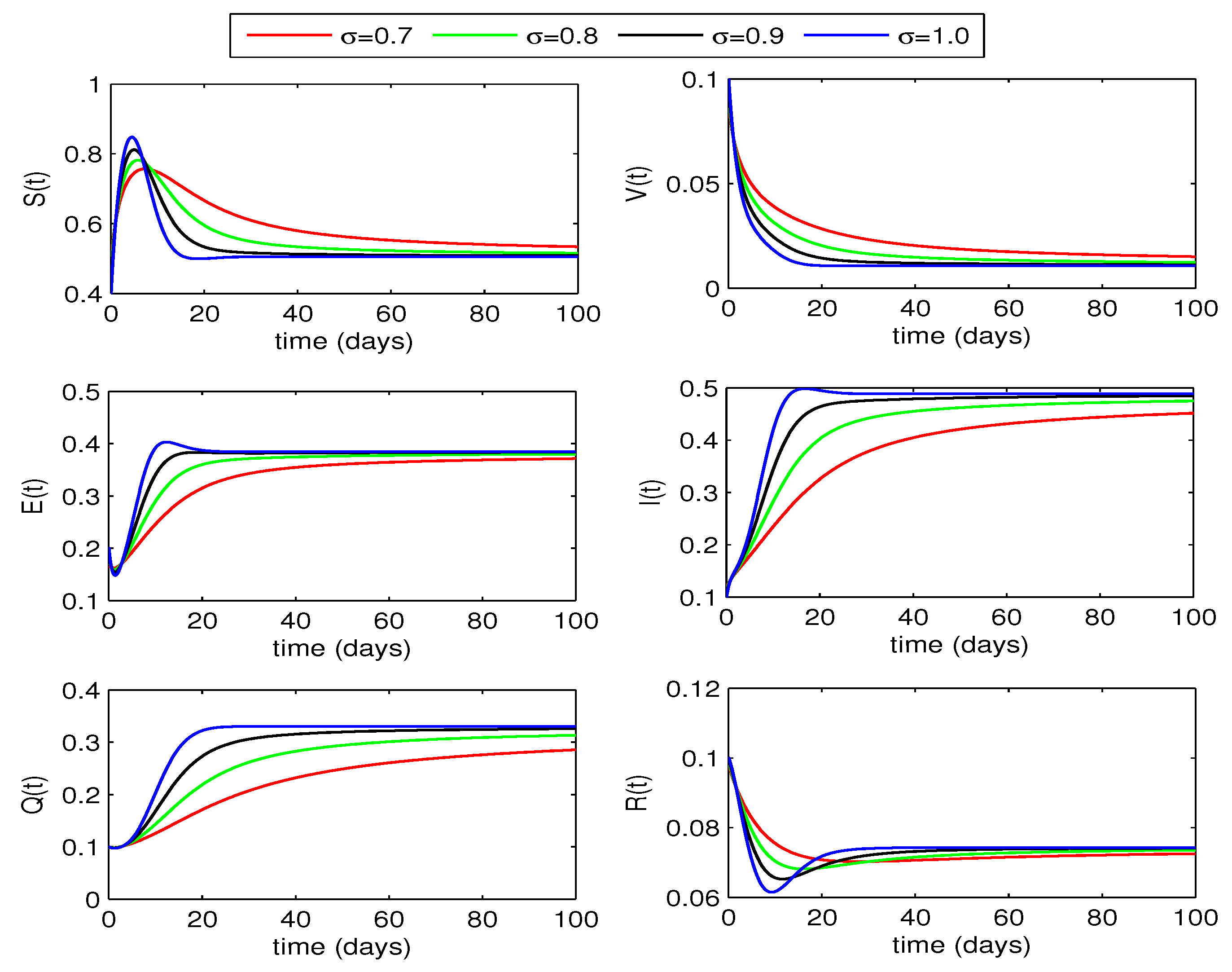
We employ the aforementioned approximations to present a graphical representation of the proposed fractional model and investigate the influence of order

σ \in (0, 1]

on solution curves.

From graphical curves of the state variables shown in Figure 2, we observe a decrease in exposed, infected and quarantined individuals with decrease in the fractional order of the differential equations. However, the susceptible increase with decrease of fractional order. Thus, reduction in fractional order values will help to reduce the whooping cough infection in humans.

4.2. Quarantining effects on disease dynamics

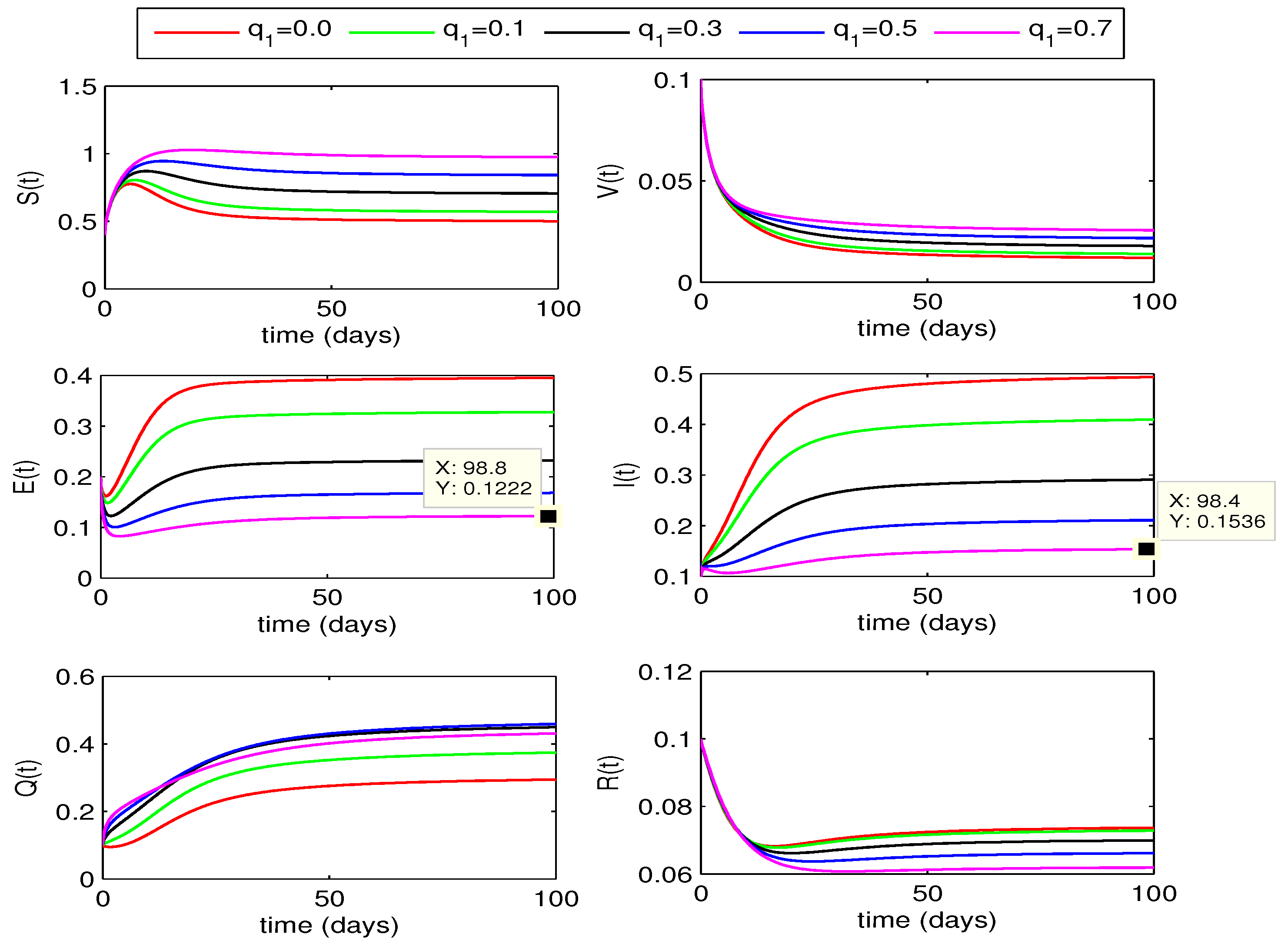
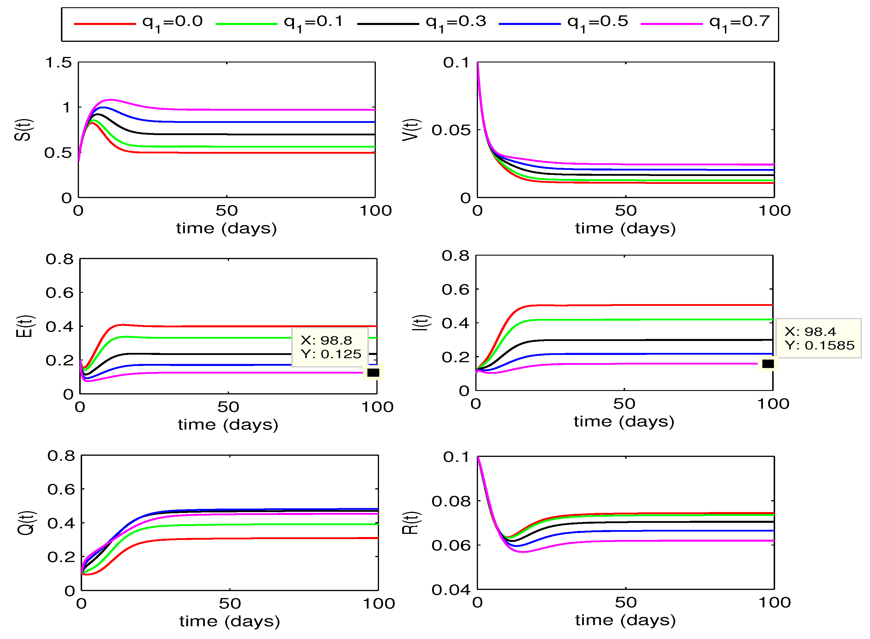
In model formulation, we had considered quarantining both of the exposed and infected individuals respectively at rates

q_{1}

and

γ_{3}

. So in this section, we study the effect of both of the rates on disease control for two different values of fractional order, i.e. for

σ = 0.8

and

σ = 0.95

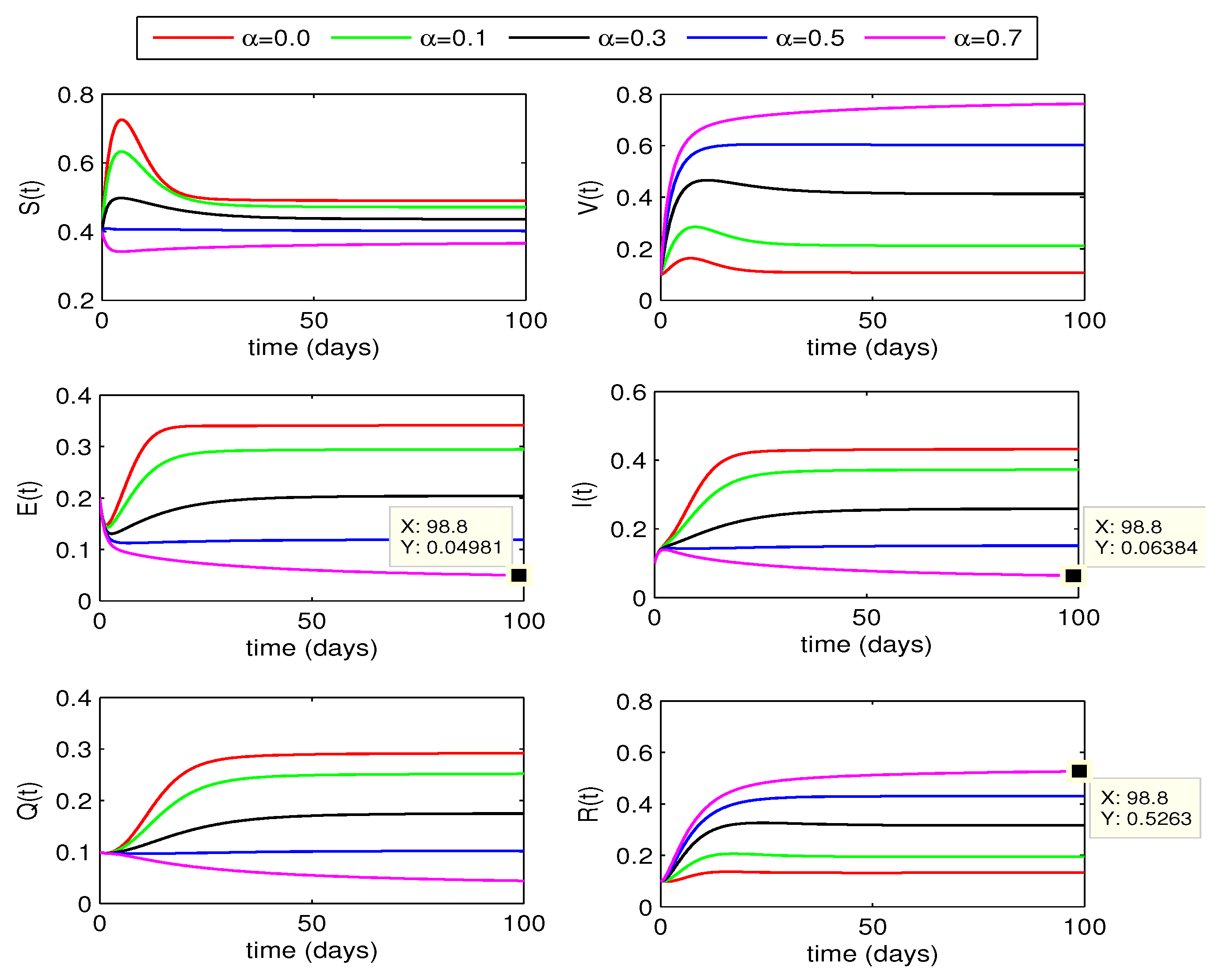
4.2.1. Effect of $q_{1}$

The impact of quarantining exposed individuals on disease dynamics can bee seen in Figure 3 and Figure 4. The curves for exposed and infected individuals decrease with increase in the quarantine rate

q_{1}

from 0 to 0.7. In this case, the recovered individuals also decrease but susceptible rise with increase in the value of

q_{1}

. We also observe that for

σ = 0.8

, the decline in infection is more as compared to the corresponding curves for fractional order

σ = 0.95

4.2.2. Effect of $γ_{3}$

The impact of quarantining infected individuals,

I (t)

, on disease dynamics can be seen in Figure 5 and Figure 6. If the quarantining rate

γ_{3}

is gradually increased up to 0.7, the curves for exposed and infected individuals gradually decrease. From this declining behavior, we may conclude that the disease may move to disease free state if the quarantining rate is increased further. Decline in infection for for fractional order

σ = 0.8

is more as compared to the case for

σ = 0.95

From the above two quarantining studies, we observe that the quarantine rate

q_{1}

has more effect in reduction of exposed cases, whereas the impact of quarantine rate

γ_{3}

is more on infected individuals.

4.3. Vaccination effect on disease dynamics

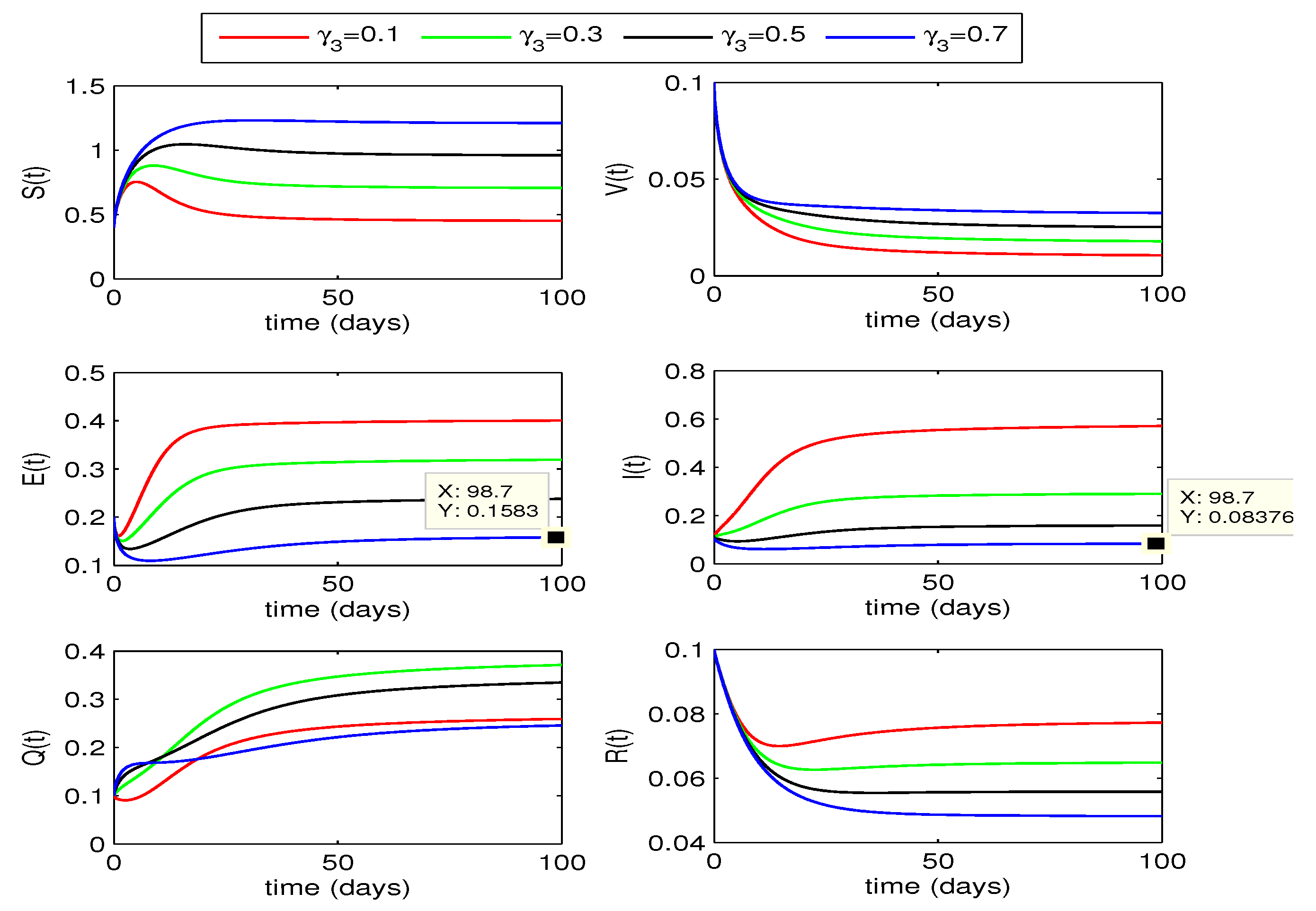
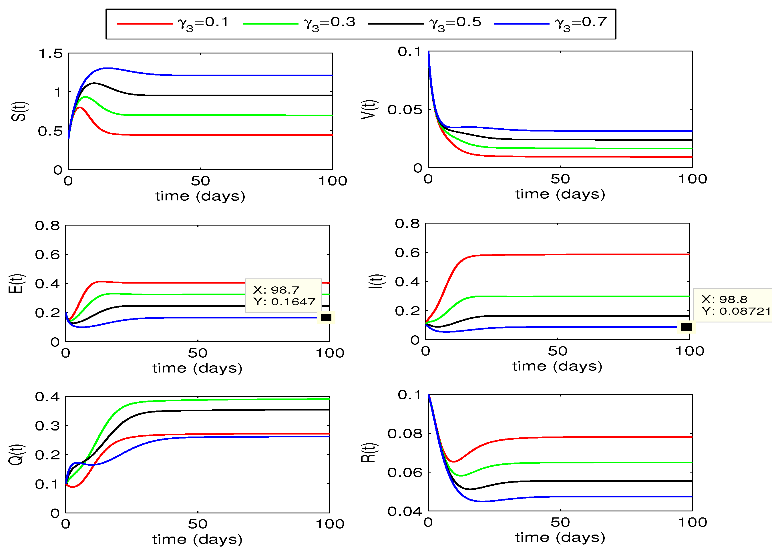
In this section, we look at how varying vaccination rates affect the dynamics of the whooping cough model quantitatively. From Figure 7 and Figure 8, we observe that the infection in population decreases as the vaccination rates increase from 0 to 0.7. If the rates are increased further, the curves for infected classes may further decline to move to disease free state. We also notice a remarkable rise in the recovered individuals in this case. The curves for exposed and infected individuals slightly decline more with increase of fractional order

σ

5. Sensitivity analysis

In this section, we find sensitivity index for each parameter of the reproduction number

R_{0}

. One the basis of these indices we determine the sensitivity of the parameter to

R_{0}

. A parameter with high index value is more sensitive to

R_{0}

. The sensitivity analysis may be helpful in designing optimal control strategies for disease control. Parameters having high sensitivity indices may be considered as control variables for the control problem.

We implement the approach given in [38] to compute sensitivity indices of the parameters of

R_{0}

. The approach is to use the following formula to compute sensitivity index of a parameter

ζ

R_{0}

I_{ζ}^{R_{0}} = \frac{\partial R_{0}}{\partial ζ} \frac{ζ}{R_{0}} .

Evaluated sensitivity indices for each parameter of

R_{0}

are listed in Table 1. Other than

Π

and

μ

, transmission rate

β

has the highest sensitivity index. Thus, this parameter is highly sensitive to

R_{0}

. A unit change in

β

will produce a change of

0.9953

R_{0}

. Other parameters having comparatively high sensitivity index are

γ

and

γ_{3}

. Since

γ_{3}

is a controllable parameter, it will be considered as one of the control variable for disease control strategy.

6. Optimization of the whooping cough model

In this section, we construct an optimal control problem with an objective to determine optimal quarantine and vaccination rates to restrict the spread of whooping cough infection. For this, we first update the disease model (5) to adjust time dependent controls and then define objective functional. We formulate Hamiltonain function by introducing adjoint variables and develop optimality conditions by implementing Pontryagin’s principle [39,40,41]. The conditions will be evaluated by following steps of an algorithm to produce optimal solutions of the control problem.

6.1. Optimal control problem and optimality conditions

The objective of defining an optimal control problem is to optimally investigate the effect of quarantining and vaccination on the spread of whooping cough disease. To achieve this objective, we formulate a control strategy for the minimization of exposed and infected individuals at a lowest cost.

First of all, we update model (5) by considering vaccination rate

α

and quarantining rates

q_{1}

γ_{3}

as time dependent controls respectively represented by

u_{1} (t), u_{2} (t)

and

u_{3} (t)

. With these controls, the updated whooping cough model is given below:

\begin{matrix} _{0}^{A B C} D_{t}^{σ} S (t) & = Π - β I S - (μ + u_{1}) S, \end{matrix}

(26a)

\begin{matrix} _{0}^{A B C} D_{t}^{σ} V (t) & = u_{1} S - δ I V - (γ_{1} + μ) V, \end{matrix}

(26b)

\begin{matrix} _{0}^{A B C} D_{t}^{σ} E (t) & = β I S + δ I V - (μ + γ + u_{2}) E, \end{matrix}

(26c)

\begin{matrix} _{0}^{A B C} D_{t}^{σ} I (t) & = γ E - (γ_{2} + u_{3} + μ + d_{1}) I, \end{matrix}

(26d)

\begin{matrix} _{0}^{A B C} D_{t}^{σ} Q (t) & = u_{2} E + u_{3} I - (q_{2} + d_{2} + μ) Q, \end{matrix}

(26e)

\begin{matrix} _{0}^{A B C} D_{t}^{σ} R (t) & = γ_{1} V + γ_{2} I + q_{2} Q - μ R, \end{matrix}

(26f)

along with conditions:

\begin{matrix} \begin{matrix} S (0) = S_{0} > 0, V (0) = V_{0} \geq 0, E (0) = E_{0} \geq 0, \\ I (0) = I_{0} \geq 0, Q (0) = Q_{0} \geq 0, R (0) = R_{0} \geq 0 . \end{matrix} \end{matrix}

(26g)

The objective functional consisting of infected states and controls is defined as:

\begin{matrix} J (z, u) = \int_{0}^{t_{f}} [a_{1} E (t) + a_{2} I (t) + \frac{1}{2} b_{1} u_{1}^{2} (t) + \frac{1}{2} b_{2} u_{2}^{2} (t) + \frac{1}{2} b_{3} u_{3}^{2} (t)] d t, \end{matrix}

(27)

where

t_{f}

is the terminal time,

z = (E, I)

represent state variables,

u = (u_{1} (t), u_{2} (t), u_{3} (t))

represent control variables,

a_{1}, a_{2}

are non-negative weights associated with state variables and

b_{i} \geq 0, i = 1, 2, 3

are cost of controls.

Our aim is to determine optimal control variable

u^{*} \in U

that minimizes the objective functional

J (z, u)

, i.e.,

\begin{matrix} min_{u (t) \in U} J (z, u) subject to model (26), \end{matrix}

(28)

where

U

is an appropriate space of control variables.

Now, we define a Hamiltonian function and implement Pontryagin’s maximum principle to derive the optimality conditions which are necessary for the solution of optimal control problem (28).

\begin{matrix} H (V (t), Ψ (t), u (t)) = & a_{1} E (t) + a_{2} I (t) + \frac{1}{2} b_{1} u_{1}^{2} (t) + \frac{1}{2} b_{2} u_{2}^{2} (t) + \frac{1}{2} b_{3} u_{3}^{2} (t) + \\ + Ψ_{1} [Π - β I S - (μ + u_{1}) S] + Ψ_{2} [u_{1} S - δ I V - (γ_{1} + μ) V] \\ + Ψ_{3} [β I S + δ I V - (μ + γ + u_{2}) E] + Ψ_{4} [γ E - (γ_{2} + u_{3} + μ + d_{1}) I] \\ + Ψ_{5} [u_{2} E + u_{3} I - (q_{2} + d_{2} + μ) Q] + Ψ_{6} [γ_{1} V + γ_{2} I + q_{2} Q - μ R], \end{matrix}

(29)

where

V (t) = (S (t), V (t), E (t), I (t), Q (t), R (t))

is a vector of state variables,

Ψ_{j} (t), j = 1, \dots, 6

are adjoint variables associated with the state equations of system (26).

Theorem 11.

[18] Let

V^{*} (t)

be the optimal solution for model (26) corresponding to optimal control variable

u^{*} (t)

for the control problem (28). Then, there exists a system of linear adjoint equations given as:

\begin{matrix} _{t}^{A B C} D_{t_{f}}^{σ} Ψ_{1} (t) = - \frac{\partial H}{\partial S}, \end{matrix}

(30a)

\begin{matrix} _{t}^{A B C} D_{t_{f}}^{σ} Ψ_{2} (t) = - \frac{\partial H}{\partial V}, \end{matrix}

(30b)

\begin{matrix} _{t}^{A B C} D_{t_{f}}^{σ} Ψ_{3} (t) = - \frac{\partial H}{\partial E}, \end{matrix}

(30c)

\begin{matrix} _{t}^{A B C} D_{t_{f}}^{σ} Ψ_{4} (t) = - \frac{\partial H}{\partial I}, \end{matrix}

(30d)

\begin{matrix} _{t}^{A B C} D_{t_{f}}^{σ} Ψ_{5} (t) = - \frac{\partial H}{\partial Q}, \end{matrix}

(30e)

\begin{matrix} _{t}^{A B C} D_{t_{f}}^{σ} Ψ_{6} (t) = - \frac{\partial H}{\partial R}, \end{matrix}

(30f)

along with the conditions:

\begin{matrix} Ψ_{1} (t_{f}) = Ψ_{2} (t_{f}) = Ψ_{3} (t_{f}) = Ψ_{4} (t_{f}) = Ψ_{5} (t_{f}) = Ψ_{6} (t_{f}) = 0, \end{matrix}

and the control variable

u^{*} (t) = (u_{1}^{*}, u_{2}^{*}, u_{3}^{*})

characterized by

\begin{matrix} u_{1}^{*} (t) & = min \{1, max \{\frac{(Ψ_{1} - Ψ_{2}) S}{b_{1}}, 0\}\}, \\ u_{2}^{*} (t) & = min \{1, max \{\frac{(Ψ_{3} - Ψ_{5}) E}{b_{2}}, 0\}\}, \\ u_{3}^{*} (t) & = min \{1, max \{\frac{(Ψ_{4} - Ψ_{5}) S}{b_{3}}, 0\}\} . \end{matrix}

Evaluation and simplification of equations (30a)-(30f) lead us to the following system of linear adjoint equations:

\begin{matrix} _{t}^{A B C} D_{t_{f}}^{σ} Ψ_{1} = & (β I + μ + u_{1}) Ψ_{1} - u_{1} Ψ_{2} - β I Ψ_{3}, \end{matrix}

(31a)

\begin{matrix} _{t}^{A B C} D_{t_{f}}^{σ} Ψ_{2} = & (δ I + γ_{1} + μ) Ψ_{2} - δ I Ψ_{3} - γ_{1} Ψ_{6}, \end{matrix}

(31b)

\begin{matrix} _{t}^{A B C} D_{t_{f}}^{σ} Ψ_{3} = & - a_{1} + (μ + γ + u_{2}) Ψ_{3} - γ Ψ_{4} - u_{2} Ψ_{5}, \\ _{t}^{A B C} D_{t_{f}}^{σ} Ψ_{4} = & - a_{2} + β S Ψ_{1} + δ V Ψ_{2} - (β S + δ V) Ψ_{3} \end{matrix}

(31c)

\begin{matrix} + (γ_{2} + u_{3} + μ + d_{1}) Ψ_{4} - u_{3} Ψ_{5} - γ_{2} Ψ_{6}, \end{matrix}

(31d)

\begin{matrix} _{t}^{A B C} D_{t_{f}}^{σ} Ψ_{5} = & (q_{2} + d_{2} + μ) Ψ_{5} - q_{2} Ψ_{6}, \end{matrix}

(31e)

\begin{matrix} _{t}^{A B C} D_{t_{f}}^{σ} Ψ_{6} = & μ Ψ_{6}, \end{matrix}

(31f)

along with the conditions

\begin{matrix} Ψ_{1} (t_{f}) = Ψ_{2} (t_{f}) = Ψ_{3} (t_{f}) = Ψ_{4} (t_{f}) = Ψ_{5} (t_{f}) = Ψ_{6} (t_{f}) = 0 . \end{matrix}

(31g)

Differentiation of Hamiltonian with respect to controls give us the expressions for controls, i.e.,

\begin{matrix} \frac{\partial H}{\partial u_{1}} = 0 \Rightarrow u_{1} (t) = \frac{Ψ_{1} - Ψ_{2}}{b_{1}} S (t), \\ \frac{\partial H}{\partial u_{2}} = 0 \Rightarrow u_{2} (t) = \frac{Ψ_{3} - Ψ_{5}}{b_{2}} E (t), \\ \frac{\partial H}{\partial u_{3}} = 0 \Rightarrow u_{3} (t) = \frac{Ψ_{4} - Ψ_{5}}{b_{3}} I (t), \end{matrix}

and the optimal characterizations for controls are given as:

\begin{matrix} u_{1}^{*} (t) & = min \{1, max \{\frac{(Ψ_{1} - Ψ_{2}) S}{b_{1}}, 0\}\}, \end{matrix}

(32a)

\begin{matrix} u_{2}^{*} (t) & = min \{1, max \{\frac{(Ψ_{3} - Ψ_{5}) E}{b_{2}}, 0\}\}, \end{matrix}

(32b)

\begin{matrix} u_{3}^{*} (t) & = min \{1, max \{\frac{(Ψ_{4} - Ψ_{5}) S}{b_{3}}, 0\}\} . \end{matrix}

(32c)

To approximate solutions of the state model (26), we employ the Toufik-Atangana method described in subSection 4.1, and for the corresponding adjoint system (31), we implement Toufik-Atangana scheme backward in time, together with the conditions (31g).

6.2. Solution algorithm

Optimality conditions for the control problem (28) are approximated for optimal solutions by following steps of the algorithm given below.

Algorithm 1:Algorithm to find minimizer of the control problem (28)

(1): Make an initial guess for control $u_{s} \in U$ for $s = 0$ .
(2): Use values of control $u_{s}$ to approximate solutions of state system (26) and adjoint system (31).
(3): Determine $u^{*}$ from (32).
(4): Refine control $u_{s}$ by using $u_{s} = (u_{s} + u^{*}) / 2$ .
(5): Stop iterations when $∥ Θ_{s} - Θ_{s - 1} ∥ < ε ∥ Θ_{s} ∥$ for $s > 0$ ,

otherwise $s + 1 ⟵ s$ and jump back to step 2.

Where

Θ

represents each of the state variables, adjoint variables and control variables and

ε > 0

is the tolerance set as per accuracy requirements.

6.3. Optimal solutions

Simulation results of the optimal control problem (28) are presented and discussed in this section. To obtain these results, we implemented steps of the Algorithm 1 through MATLAB code. We discretize the domain

[0, t_{f}]

into

N + 1

discrete points

t_{q} = q h, q = 0, 1, \dots, N

where

h = \frac{t_{f}}{N}

and approximate the state and adjoint equations using the approximating scheme, explained in Section 4.1. We use Simpson’s rule to approximate the cost functional (27) at the discrete points. Results are simulated for different values of fractional order, i.e., for

σ = 0.75, 0.8, 0.9, 1

The objective of this study is to determine the optimal quarantine rates

q_{1}

γ_{3}

and the vaccination rate

α

that will not only minimize the cost functional but will also reduce the whooping cough infection in the society. For detailed analysis, we discuss here three different cases. In the first case, we keep quarantine rates

q_{1}

γ_{3}

fix in time and determine the optimal vaccination rate

α (t)

for disease control. In second case, we determine the best quarantine rates

q_{1} (t)

γ_{3} (t)

that will reduce the spread of whooping cough infection. In this case, vaccination rate will be considered as time independent. In the last strategy, we deal with time-dependent vaccination rate and quarantine rates together to determine their optimal profiles that will help to reduce the cost functional to its minimum and to curtail the whooping cough disease infection.

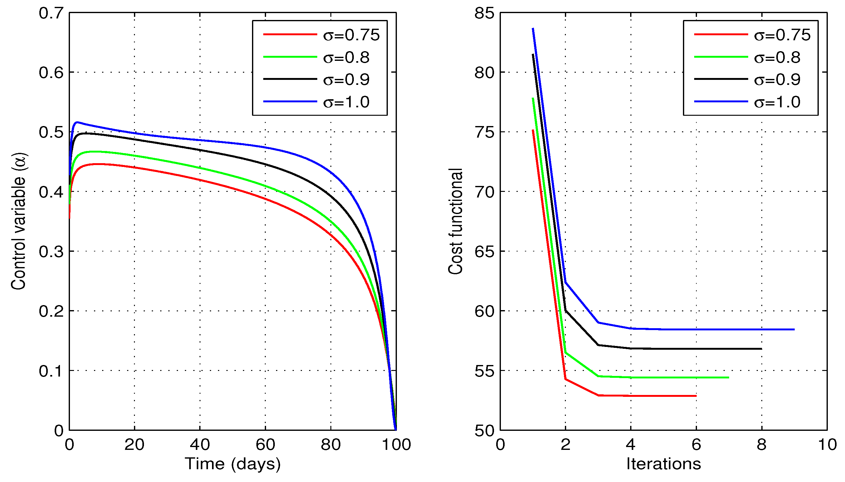
6.3.1. Optimal vaccination rate

In the first case, we consider optimization of the problem (28) by considering only vaccination rate

α (t) (= u_{1} (t))

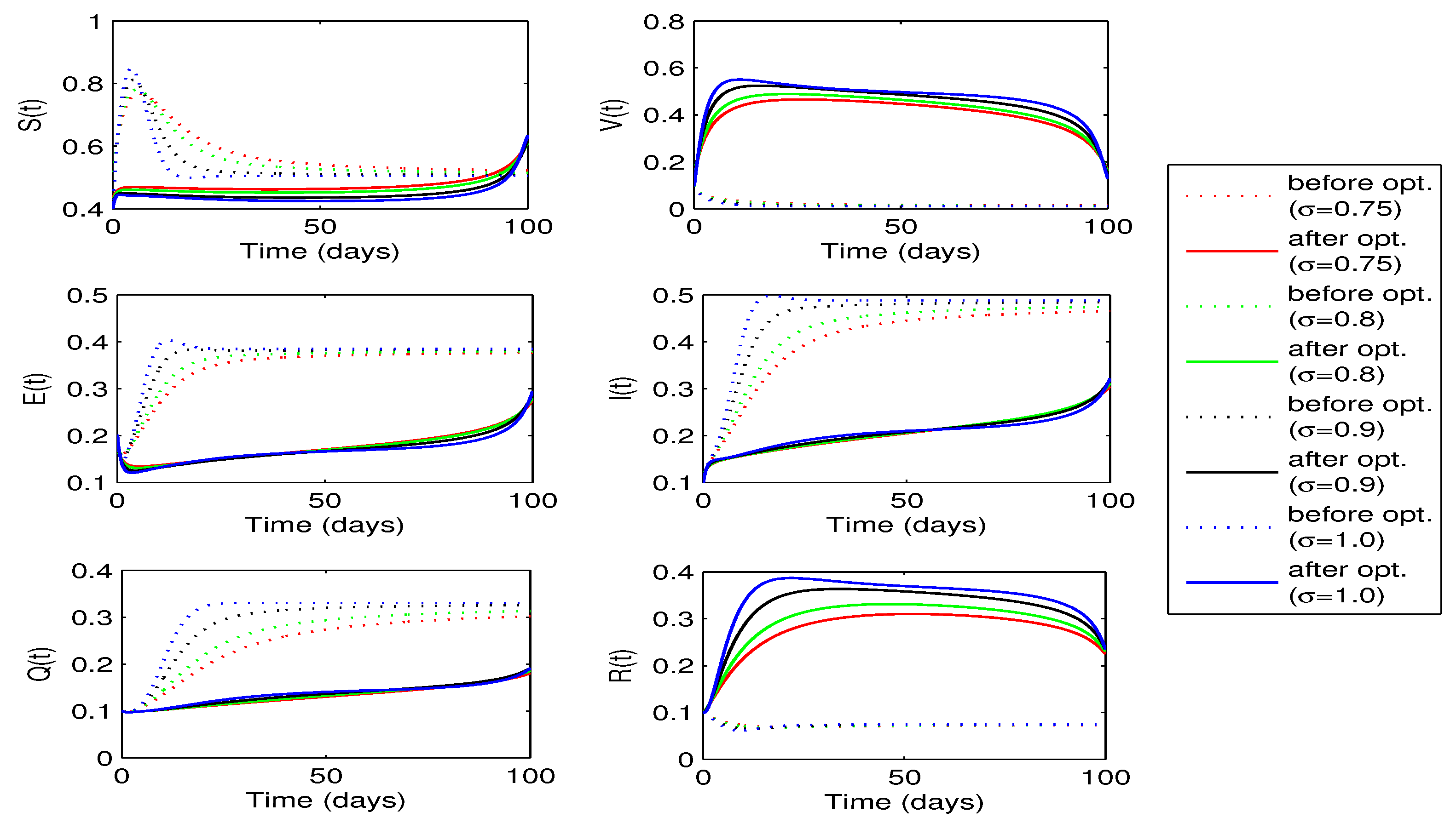
as the time dependent control variable. Figure 9 shows profiles of the optimal vaccination rate

α (t)

and the associated cost functional J for different values of fractional order

σ

. We observe that the cost functional has attained its minimum for each value of the considered fractional order

σ

. The behaviors of state variables before and after optimization for each value of the fractional order

σ

are shown in Figure 10. A sufficient decrease in the exposed and infected individuals is noticed in this figure, however, there is a significant rise in the recovered individuals. Thus, the strategy is successful in reducing the disease infection and increasing the recovered individuals.

6.3.2. Optimal quarantine rates

Now, we take quarantine rates

q_{1} (t) (= u_{2} (t))

and

γ_{3} (t) (= u_{3} (t))

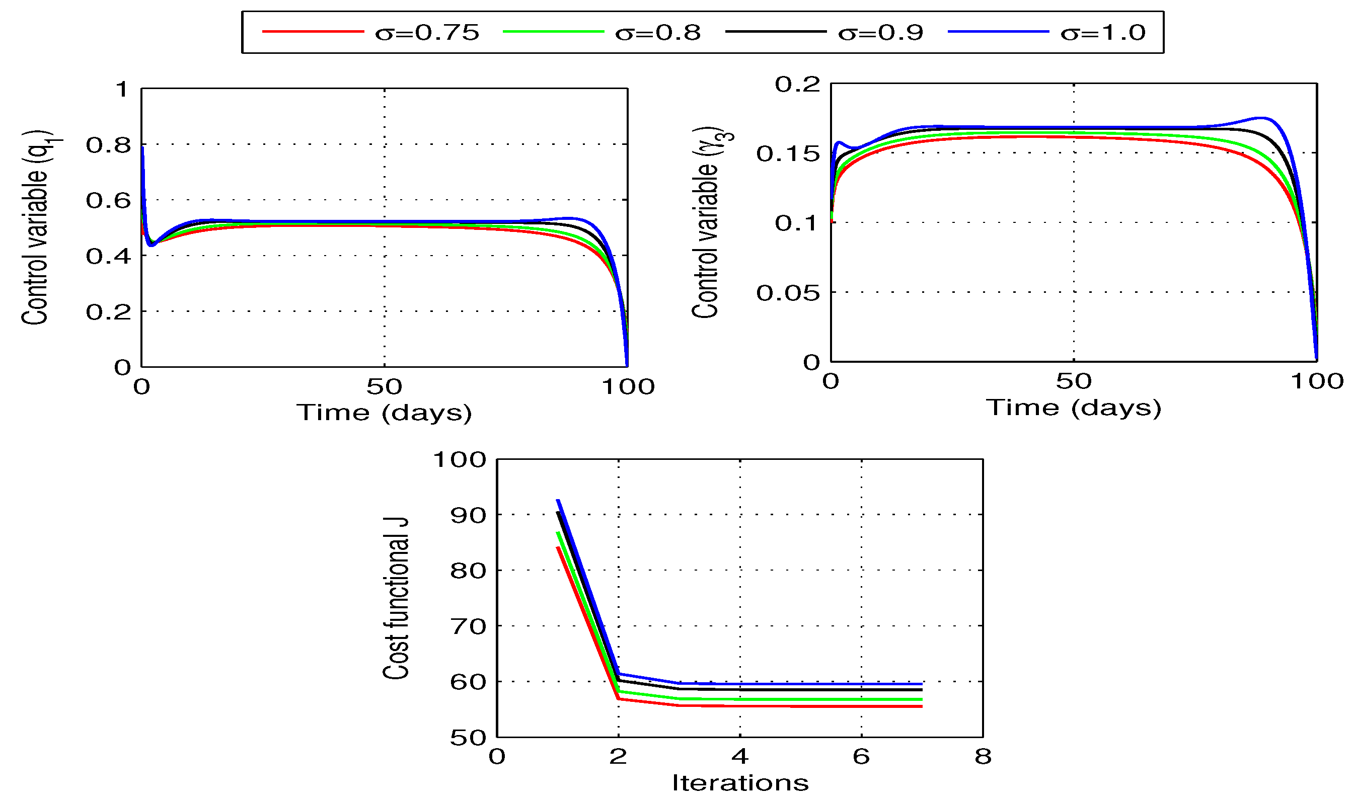
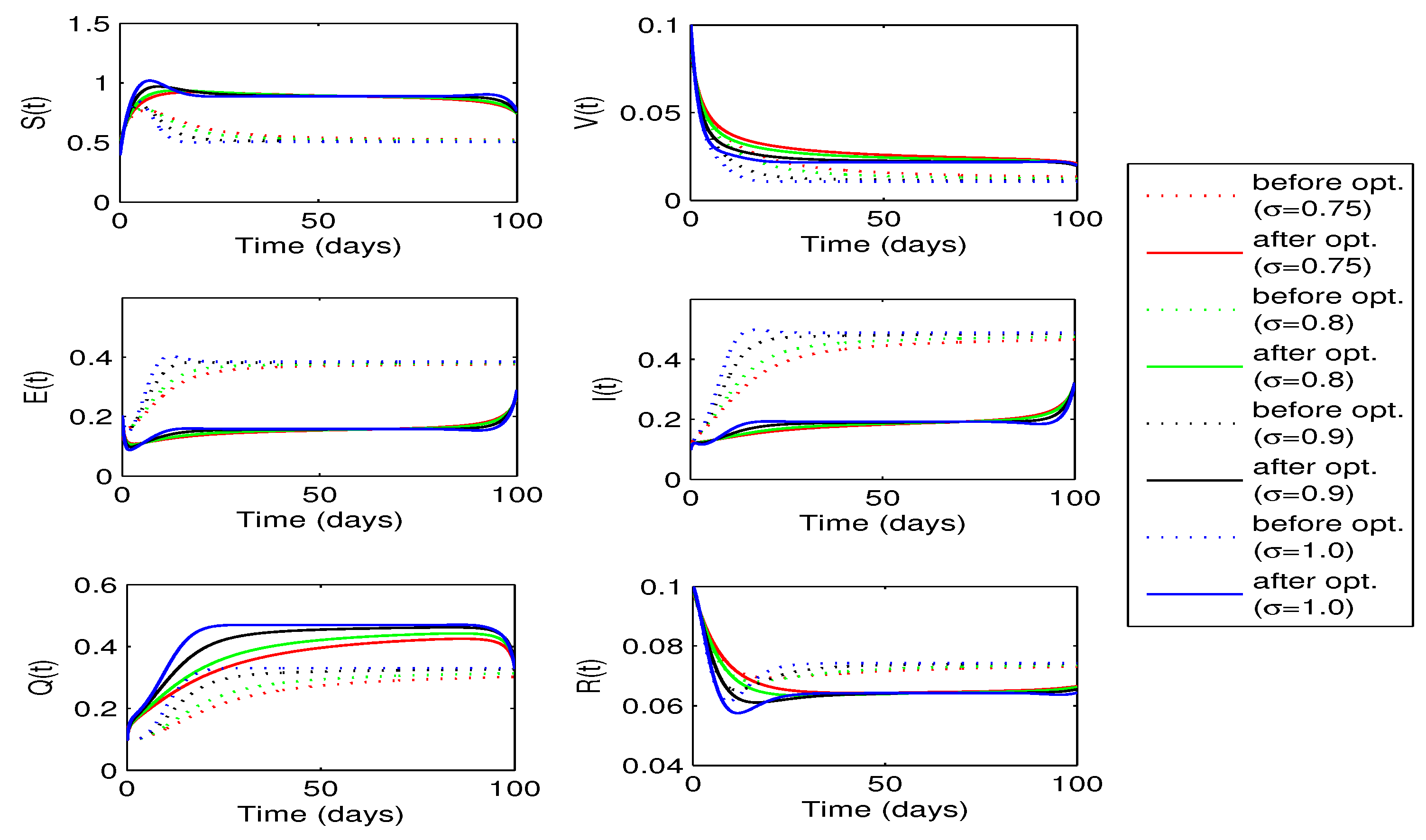
as the time dependent control variables for the problem (28). Optimal curves for the control variables and the corresponding behavior of cost functional for different values of fractional order are shown in the Figure 11. In each case, the curves for cost functional reaches to their minimum in seven iterations. Figure 12 shows the curves for state variables before and after optimization. Once again we observe a decrease in the number of exposed and infected individuals in this case. However, decrease in this case is slightly more as compared to the when only vaccination rate

α (t)

is considered as a single control variable. We also notice a decrease in the number of recovered individuals but increase in the susceptibles for each value of fractional order

σ

6.3.3. Optimal vaccination and quarantine rates

In the last case, we consider vaccination rate

α (t)

and the quarantine rates

q_{1} (t), γ_{3} (t)

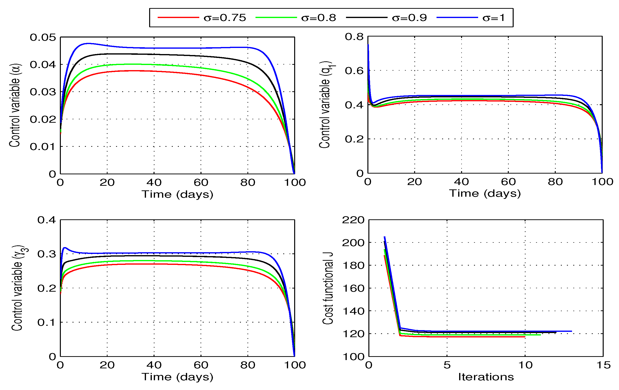
as control variables for the optimal control problem (28). For this case, optimal behavior of the control variables and minimization of the related objective functional J are shown in Figure 13. In this case, the cost functional reduces to its minimum in different number of iterations for different values of fractional order

σ

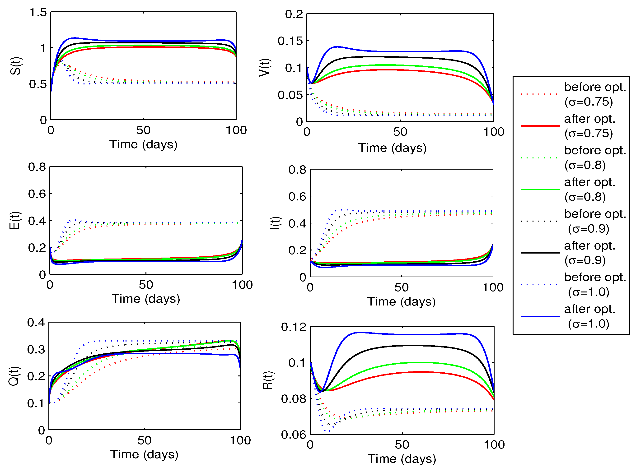
. However, cost functional takes more iterations to reach minimum value as compared to the last two considerations. Profiles of state variables before and after optimization are shown in Figure 14. Number of exposed and infected individuals decrease more in this case as compared to the previous two optimal cases. We also notice a sufficient rise in the susceptible and recovered curves for each given value of the fractional order

σ

The analysis of the three cases reveals that considering all the three controls together is more effective in reducing the infection of whooping cough disease. However, implementation of this strategy requires more resources and infrastructure as compared to the first two cases.

7. Conclusions

In this work, we formulated a new ABC fractional disease model for whooping cough infection to analyze dynamics of the disease and to suggest optimal control strategies for minimizing effect of the disease. First of all, we analyzed the model theoretically by establishing biologically significant aspects of the model. We proved that the proposed model has a unique solution which is positive and bounded. It is also verified that the equilibrium points are locally and globally stable with restriction to threshold parameter

R_{0}

. These results concluded that the proposed model is well-posed for further numerical investigations. Through sensitivity analysis, we determined that the disease transmission rates

β

and

γ

, and the quarantine parameter

γ_{3}

are the most sensitive parameters to

R_{0}

. Due to their significant impact on

R_{0}

, the parameters may be considered as control variable for optimal control analysis.

Another objective of this study was to suggest an optimal control strategy to restrict the spread of whooping cough infection. For this, we considered vaccination rate

α

and quarantine rates

q_{1}

(E

Q)

γ_{3}

(I

Q)

as control variables and studied their impact on disease control. First of all, we took different levels (0 to 0.7) of these parameters and explored impact of each on disease control. We determined that the disease can be controlled significantly by increasing values of these parameters. However, it is concluded that vaccination of susceptible is more effective as compared to quarantining the exposed or infected individuals. The impact of memory index (fractional order)

σ

on disease dynamics was also investigated here. We visualized a decrease in the infection cases with a decrease in the memory index.

For optimal control analysis, we considered the parameters

α, q_{1}

and

γ_{3}

as time dependent controls and formulated an optimal control problem by defining a cost functional. The aim was to determine optimal values of the control variables that minimize the cost functional. By implementing Pontryagin’s principle, we derived necessary optimality conditions for optimal solution of the problem. In this study, we discussed three different optimal control approaches. In the first case, we determined optimal solutions by considering only vaccination rate

α

as the control variable. In the second approach, we considered quarantine rates

q_{1}, γ_{3}

as the time-dependent controls and determined optimal solutions for the given problem. In the last case, all the three parameters

α, q_{1}, γ_{3}

were taken as time-dependent controls for optimal solutions. Graphical results show that each of the considered strategy is very much effective in reducing the exposed and infected individuals and hence may be implemented to reduce the whooping cough infection from the society. The graphical results also revealed that the case where we have considered all the three controls together is more effective in reducing the spread of whooping cough infection. However, implementation of this approach requires more resources and infrastructure as compared to the other two cases. It is also concluded that the simulation results through time-dependent controls are more cost-effective as compared to the results produced by time-independent controls. In future, a Covid-19 and whooping cough co-infection model may be developed and explored for various optimal control strategies with cost-effective analysis.

Funding

Funding is not available so far.

Sample Availability

The data is given with in the article.

References

H. Bokhari, F. Said, M. A. Syed, A. Mughal, Y. F. Kazi, K. Heuvelman and F. R. Mooi, Whooping cough in Pakistan- Bordetella Pertussis vs Bordetella Parapertussis in 2005-2009, Scandanavian Journal of Infectious Disease 47, No. 2 (2011) 01-03.
H. R. Joshi, S. Lenhart, M. Y. Li and L. Wang, Optimal control methods applied to disease models in the mathematical studies on human disease dynamics, Contemporary Mathematics 410, (2006) 187-207.
CDC report on Pertussis (Whooping Cough) in Other Countries, https://www.cdc.gov/pertussis/countries/index.html. Available online: https://www.cdc.gov/pertussis/countries/index.html.
S. Obaidat, M.R.A. Elrish, S. Mesloub, A second order scheme for the numerical solution of a whooping cough model, Journal of Computational and Theoretical Nanoscience, 14(9):4352-4360, 2017.
L.A. Van Bellinghen, A. Dimitroff, M. Haberl et.al., Is adding maternal vaccination to prevent whooping cough cost effective in Australia? Human Vaccines and Immunotherapeutics, 14(9), 2263-2277, 2018, doi: 10.1080/21645515.2018.1474315. [CrossRef]
M. Suleman, An optimal control of vaccination applied to whooping cough model, Journal of Mathematics, 51:121-136, 2019.
K. Ameri, K.D. Cooper, A Network-Based compartmental model for the spread of whooping cough in Nebraska, AMIA Summits on Translational Science Proceedings, Vol. 388, 2019.
M.M. Algarni, Arooj Nasir, M.A. Alyami, A. Raza, et. al., A SEIR epidemic model of whooping cough-like infections and its dynamically consistent approximation, Hindawi Complexity, Volume 2022, Article ID:3642444.
R.M. Jena, S. Chakraverty, S. K. Jena, Analysis of the dynamics of phytoplankton nutrient and whooping cough models with nonsingular kernel arising in the biological system, Chaos, Solitons and Fractals, 141, 2020, 110373,https://doi.org/10.1016/j.chaos.2020.110373. [CrossRef]
K. Diethelm, A fractional calculus based model for the simulation of an outbreak of dengue fever, Nonlinear Dynam., 71 (2013), 613–619. https://doi.org/10.1007/s11071-012-0475-2. [CrossRef]
M. A. Khan, S. Ullah, M. Farooq, A new fractional model for tuberculosis with relapse via Atangana-Baleanu derivative, Chaos Soliton. Fract., 116 (2018), 227–238. https://doi.org/10.1016/j.chaos.2018.09.039. [CrossRef]
S. Ullah, M. A. Khan, M. Farooq, A fractional model for the dynamics of tuberculosis virus, Chaos Soliton. Fract., 116 (2018), 63–71. https://doi.org/10.1016/j.chaos.2018.09.001. [CrossRef]
H. W. Berhe, S. Qureshi, A. A. Shaikh, Deterministic modeling of dysentery diarrhea epidemic under fractional Caputo differential operator via real statistical analysis, Chaos Soliton. Fract., 131 (2020), 109536, https://doi.org/10.1016/j.chaos.2019.109536. [CrossRef]
S. Qureshi, Z. N. Memon, Monotonically decreasing behavior of measles epidemic well captured by Atangana-Baleanu-Caputo fractional operator under real measles data of Pakistan, Chaos Soliton. Fract., 131 (2020), 109478,https://doi.org/10.1016/j.chaos.2019.109478. [CrossRef]
A. I. K. Butt, W. Ahmad, M. Rafiq, D. Baleanu, Numerical analysis of Atangana-Baleanu fractional model to understand the propagation of a novel corona virus pandemic, Alexandria Engineering Journal. (2022) 61, 7007-7027.
A.I.K. Butt, M. Imran, S. Batool, M. AL Nuwairan, Theoretical Analysis of a COVID-19 CF-Fractional Model to Optimally Control the Spread of Pandemic, Symmetry. (2023), 15, 380. https:// doi.org/10.3390/sym15020380. [CrossRef]
Asma Hanif, A.I.K. Butt, W. Ahmad, Numerical approach to solve Caputo-Fabrizio fractional model of corona pandemic with optimal control design and analysis, Mathematical Methods in the Applied Sciences. (2023) 1-32, https://doi.org/10.1002/mma.9085. [CrossRef]
Asma Hanif, A.I.K. Butt, Atangana-Baleanu fractional dynamics of dengue fever with optimal control strategies, AIMS Mathematics. (2023), 8(7): 15499–15535, doi: 10.3934/math.2023791. [CrossRef]
J. K. K. Asamoah, Fractal fractional model and numerical scheme based on Newton polynomial for Q fever disease under Atangana-Baleanu derivative, Results Phys., 34 (2022). https://doi.org/10.1016/j.rinp.2022.105189. [CrossRef]
D. Baleanu, A. Jajarmi, H. Mohammadi, S. Rezapour, A new study on the mathematical modelling of human liver with Caputo-Fabrizio fractional derivative, Chaos, Solitons & Fractals. 134 (2020) 109705.
D. Baleanu, F. Akhavan Ghassabzade, J.J. Nieto, A. Jajarmi, On a new and generalized fractional model for a real cholera outbreak, Alexandria Engineering Journal. 61(11) (2022) 9175-9186.
Ali, I., Khan, S.U, Threshold of Stochastic SIRS Epidemic Model from Infectious to Susceptible Class with Saturated Incidence Rate Using Spectral Method, Symmetry. (2022), 14, 1838. https://doi.org/10.3390/sym14091838. [CrossRef]
Ishtiaq Ali, Sami Ullah Khan, Dynamics and simulations of stochastic COVID-19 epidemic model using Legendre spectral collocation method, AIMS Mathematics. (2023), Volume 8, Issue 2: 4220-4236. doi: 10.3934/math.2023210. [CrossRef]
A.I.K. Butt, S. Batool, M. Imran, M. AL Nuwairan, Design and analysis of a new COVID-19 model with comparative study of control strategies, Mathematics. (2023) 11(9) 1978; https://doi.org/10.3390/ math11091978. [CrossRef]
A.I.K. Butt, D.B.D. Chamaleen, S. Batool, M. AL Nuwairan, A new design and analysis of optimal control problems arising from COVID-19 outbreak, Math Meth Appl Sci. (2023), https://doi.org/10.1002/mma.9482. [CrossRef]
A.I.K. Butt, M. Rafiq, W. Ahmad, N. Ahmad, Implementation of a computationally efficient numerical approach to analyze a Covid-19 pandemic model, Alexandria Engineering Journal. 69(2023), 341-362, 2023. https://doi.org/10.1016/j.aej.2023.01.052. [CrossRef]
Begum, Razia; Tunç, Osman; Khan, Hasib; Gulzar, Haseena; Khan, Aziz A fractional order Zika virus model with Mittag-Leffler kernel, Chaos Solitons Fractals. 146 (2021), Paper No. 110898, 11 pp.
A. Atangana, D. Baleanu, New fractional derivatives with nonlocal and non-singular kernel: theory and application to heat transfer model, Thermal Science, 2016; 20(2):763-9.
A. Atangana, I. Koca, Chaos in a simple nonlinear system with Atangana-Baleanu derivative with fractional order, Chaos Solitons and Fractals, vol. 89, pp:447-454, 2016.
E. Kreyszig, Introductry functional analysis with application, John Wiley and Sons, New York, 1993.
V. I. Arnold, Ordinary differential equations, MIT Press, London, UK, 1998.
A. Atangana, D. Baleanu, New fractional derivatives with nonlocal and non-singular kernel: Theory and application to heat transfer model, Therm. Sci., 20 (2016), 763–769. https://doi.org/10.2298/TSCI160111018A. [CrossRef]
O. Diekmann, J. A. P. Heesterbeek, and J. A. Metz, On the definition and the computation of the basic reproduction ratio R0 in models for infectious diseases in heterogeneous populations, J. Math. Biol. 28 (1990), 365–382.
W. Ahmad, M. Rafiq, M. Abbas, Mathematical analysis to control the spread of Ebola virus epidemic through voluntary vaccination, European Physical Journal Plus. (2020), vol. 135, Issue 10, Article no. 775, pp: 1-34.
Castillo-Chavez, C., Feng, Z., Huanz, W., Driessche, P.V.D., Kirschner, D.E. On the computation of R₀ and its role in global stability, In Mathematical Approaches for Emerging and Reemerging Infectious Diseases: An Introduction; Springer: Berlin/Heidelberg, Germany (2002).
M. Toufik, A. Atangana, New numerical approximation of fractional derivative with nonlocal and non-singular kernel: Application to chaotic models, Eur. Phys. J. Plus, 132 (2017). https://doi.org/10.1140/epjp/i2017-11717-0. [CrossRef]
M. A. Khan, A. Atangana, Modeling the dynamics of novel coronavirus (2019-nCov) with fractional derivative, Alex. Eng. J., 59 (2020), 2379–2389. https://doi.org/10.1016/j.aej.2020.02.033. [CrossRef]
Pauline Van Den Drissche, Reproduction numbers of infectious disease models, Infectious Disease Modelling. (2017) 2,288-303.
R. Kamocki, Pontryagin maximum principle for fractional ordinary optimal control problems, Math. Method. Appl. Sci., 37 (2014), 1668–1686. https://doi.org/10.1002/mma.2928. [CrossRef]
S. Lenhart, J. T. Workman, Optimal control applied to biological models, CRC Press, 2007.
H. M. Ali, F. L. Pereira, S. M. Gama, A new approach to the Pontryagin maximum principle for nonlinear fractional optimal control problems, Math. Method. Appl. Sci., 39 (2016). https://doi.org/10.1002/mma.3811. [CrossRef]

Figure 1. Flow diagram of whooping cough disease transmission.

Figure 2. Dynamics of the state variables of whooping cough epidemic model for different values of fractional order

σ

Figure 2. Dynamics of the state variables of whooping cough epidemic model for different values of fractional order

σ

Figure 3. Effect of quarantine rate

q_{1}

on state variables with

σ = 0.8

Figure 3. Effect of quarantine rate

q_{1}

on state variables with

σ = 0.8

Figure 4. Effect of quarantine rate

q_{1}

on state variables with

σ = 0.95

Figure 4. Effect of quarantine rate

q_{1}

on state variables with

σ = 0.95

Figure 5. Effect of quarantine rate

γ_{3}

on state variables with

σ = 0.8

Figure 5. Effect of quarantine rate

γ_{3}

on state variables with

σ = 0.8

Figure 6. Effect of quarantine rate

γ_{3}

on state variables with

σ = 0.95

Figure 6. Effect of quarantine rate

γ_{3}

on state variables with

σ = 0.95

Figure 7. Effect of vaccination rate

α

on state variables with

σ = 0.8

Figure 7. Effect of vaccination rate

α

on state variables with

σ = 0.8

Figure 8. Effect of vaccination rate

α

on state variables with

σ = 0.95

Figure 8. Effect of vaccination rate

α

on state variables with

σ = 0.95

Figure 9. Optimal vaccination rate

α

and the cost functional J for different values of fractional order

σ

Figure 9. Optimal vaccination rate

α

and the cost functional J for different values of fractional order

σ

Figure 10. State variables before and after optimization with vaccination rate

α (t)

as control variable.

Figure 10. State variables before and after optimization with vaccination rate

α (t)

as control variable.

Figure 11. Optimal quarantine rates

q_{1} (E

Q)

γ_{3} (I

Q)

and the cost functional J for different values of fractional order

σ

Figure 11. Optimal quarantine rates

q_{1} (E

Q)

γ_{3} (I

Q)

and the cost functional J for different values of fractional order

σ

Figure 12. State variables before and after optimization with quarantine rates

q_{1} (t), γ_{3} (t)

as control variables.

Figure 12. State variables before and after optimization with quarantine rates

q_{1} (t), γ_{3} (t)

as control variables.

Figure 13. Optimal vaccination rate

α (t)

, quarantine rates

q_{1} (E

Q)

γ_{3} (I

Q)

and the cost functional J for different values of fractional order

σ

Figure 13. Optimal vaccination rate

α (t)

, quarantine rates

q_{1} (E

Q)

γ_{3} (I

Q)

and the cost functional J for different values of fractional order

σ

Figure 14. State variables before and after optimization with vaccination and quarantine rates

α (t), q_{1} (t), γ_{3} (t)

as control variables.

Figure 14. State variables before and after optimization with vaccination and quarantine rates

α (t), q_{1} (t), γ_{3} (t)

as control variables.

Table 1. Sensitivity indices for each parameter of

R_{0} .

Table 1. Sensitivity indices for each parameter of

R_{0} .

Parameter	Sensitivity Index	Parameter	Sensitivity Index
$Π$	1.0000	$μ$	-1.8150
$α$	-0.0388	$β$	0.9953
$δ$	0.0046	$γ$	0.3243
$γ_{1}$	-0.0018	$γ_{2}$	-0.0507
$γ_{3}$	-0.3807	$q_{1}$	-0.0270
$d_{1}$	-0.0101	$d_{2}$	0.0000

Disclaimer/Publisher’s Note: The statements, opinions and data contained in all publications are solely those of the individual author(s) and contributor(s) and not of MDPI and/or the editor(s). MDPI and/or the editor(s) disclaim responsibility for any injury to people or property resulting from any ideas, methods, instructions or products referred to in the content.

© 2023 by the authors. Licensee MDPI, Basel, Switzerland. This article is an open access article distributed under the terms and conditions of the Creative Commons Attribution (CC BY) license (http://creativecommons.org/licenses/by/4.0/).

Copyright: This open access article is published under a Creative Commons CC BY 4.0 license, which permit the free download, distribution, and reuse, provided that the author and preprint are cited in any reuse.

MDPI Initiatives

Important Links

Choose an area of interest and we will send you notifications of new preprints at your preferred frequency.

Disclaimer

Atangana-Baleanu fractional dynamics of predictive whooping cough model with optimal control analysis

Abstract

1. Introduction

2. Model formulation

2.1. Fractional model

3. Theoretical analysis of the proposed model

3.1. Existence and uniqueness of solution

3.2. Boundedness and positivity of the solutions

3.3. Equilibrium points and threshold parameter R 0

3.3.1. Disease free equilibrium point

3.3.2. Reproduction number

3.3.3. Endemic equilibrium

3.4. Stability analysis

3.4.1. Local stability

3.4.2. Global stability

4. Numerical investigations and implementations

4.1. Toufik-Atangana discretizations

4.1.1. Fractional order effect on disease dynamics

4.2. Quarantining effects on disease dynamics

4.2.1. Effect of q 1

4.2.2. Effect of γ 3

4.3. Vaccination effect on disease dynamics

5. Sensitivity analysis

6. Optimization of the whooping cough model

6.1. Optimal control problem and optimality conditions

6.2. Solution algorithm

6.3. Optimal solutions

6.3.1. Optimal vaccination rate

6.3.2. Optimal quarantine rates

6.3.3. Optimal vaccination and quarantine rates

7. Conclusions

Funding

Sample Availability

References

MDPI Initiatives

Important Links

Subscribe

3.3. Equilibrium points and threshold parameter $R_{0}$

4.2.1. Effect of $q_{1}$

4.2.2. Effect of $γ_{3}$