
Submitted:
02 August 2023
Posted:
03 August 2023
You are already at the latest version
Abstract
Currently, a wide variety of velocity profiles are used in motion control. Thus, this paper compares the energy consumption of three parabolic, trapezoidal, and S-curve profiles. We studied the case of using embedded systems since they are a powerful solution to monitor and coordinate the movement of devices and machinery in various industries combined with motion control applications. These integrated systems allow precise and efficient control of motors and actuators through control and feedback algorithms. In addition, we propose an alternative methodology for implementing motion controllers using an Advanced RISC Machine (ARM) microcontroller, which computes the trajectory and the control action in real-time. We conducted an experiment using a linear plant composed of a direct current (DC) motor coupled to an endless screw where a carriage is mounted that can move mechanically along a rail a distance of 1.16m. In addition, a 4096 pulses per revolution (PPR) encoder is connected to the motor to measure position and angular velocity, which compute the distance the carriage has moved in meters. A current sensor is used to assess the energy consumption, and 40 tests for each profile were carried out to compare the energy consumption for the three-motion profiles considering cases with and without load on the carriage.
Keywords:
power consumption
; trapezoidal profile
; parabolic profile
; S-Curve
; embedded systems
; microcontroller
1. Introduction
Scientist have been studied extensively motion profiles for several decades, since it has uncountable applications related to motion control, robotics, and commercial machinery, such as robot manipulators [1,2], conveyor belts, computer numerical control (CNC) machinery, 3D printers, and any system that needs to control movement based on electric motors [3,4,5]. The motion profiles define not only the position of the motor shaft but also the velocity, acceleration, and the third derivative of position (jerk) along the path or entire movement [6]. With constant movement phases, it is possible to generate smooth trajectories that reduce mechanical wear and aggressive current peaks to improve movements’ precision [7,8]. So, motion profiles are focused on obtaining a function of time, which returns at each instant the position that the mechanical system must follow [9]. Constantly it is sought to have at least continuous acceleration [10], since discontinuities in acceleration, such as in a trapezoidal profile, can cause the jerk to be too large and residual vibrations are generated [11], which, in addition to affecting the precision of the movement, also degrade valuable life of the mechanical system [12]. On the other hand, in mechatronics systems, motion profiles are applied to execute point-to-point movements [13]. For instance, to move from an initial point to a final point, the trajectory must be smooth, according to the cinematic magnitude restrictions of the system, with which an exceeding of the speed, acceleration, or jerk limits supported by the motor is avoided [14].
Another aspect to consider besides the motion profiles is the control algorithm , which is designed to keep the tracking error as low as possible, guaranteeing efficiency in the execution of the movement [15]. The most commonly used control technique is the classical Proportional-Integral-Derivative (PID) and PD controllers as observed in [16]. However, technological changes demand new control strategies that present a better response than traditional controllers. For example, in [17], the implementation of a controller based on fuzzy logic for a robot manipulator shows better performance in terms of robustness and trajectory following; in [18] an adaptive controller with neural networks is used, which improves the precision of the movement at the cost of greater computational demands.
In recent years, several works have been proposed that allow smooth movements to be executed using functions of the polynomial, exponential, trigonometric type, or a combination of these [19,20,21,22]. The study of the motion profiles has shown that, depending on the path implemented, it is possible to minimize execution times, reduce vibrations by minimizing the jerk (which translates into less wear on the mechanical structure), as well as reduce energy consumption [23]. Fang Y. et al. use a 15-segment s-curve trajectory formed by pieces of sigmoid functions, which allows for obtaining successive continuous derivatives [24]. This results in a trajectory with vibration and reduced tracking error verified experimentally in a robotic arm. Similarly, Wu et al. propose a 15-segment trajectory with a shorter execution time. It is made up of pieces of functions of the trigonometric type, with constant motion phases [1]. Alpers employs a 7-segment motion profile based on chunks of polynomial functions [25]. However, discontinuities in successive derivatives can cause unwanted vibrations; [10] proposes an improvement with a 15-segment path, in which the snap is a continuous piece-wise function; Due to the complexity of the expressions, the time required to calculate the trajectory is longer compared to classical profiles. Lee and Han use nth-order polynomial motion profiles to achieve fast motion and minimal vibration in an industrial robot [12]; the motion controller is implemented on a 32-bit MCU. Jerk minimization has been achieved through the use of degree 7 polynomials, as shown by Wu and Zhang in [4], which is implemented in a robot manipulator. Similarly, Boryga et al. use polynomials of degrees 5 to 9 to obtain phases of continuous motion [3]. However, experimental results still need to be presented. For their part, Wang H. et al. propose a methodology for using degree 4 polynomials in an industrial robot [26]. On the other hand, the reduction of energy consumption has been analyzed in point-to-point movements using trapezoidal and cycloid profiles [2], as well as trajectories based on Chebyshev polynomials [15]. A review and classification on energy-saving optimization strategies for robotic and automatic systems is presented in [27], being the software approach based on the motion planning an effective and economical technique easy to implement on existing system [28]. Montalvo et al. conducted a comparative analysis of the energy consumption of the trapezoidal and parabolic motion profiles on a Field-Programmable Gate Array (FPGA)-based motion control system [29]. A similar study was conducted by Carabani G. and Vidoni R. adding higher-order polynomial and modified s-curve profiles [30], however, Hosseini, S., and Hahn obtained better energy saving with third-degree polynomials than with higher degree trajectories [31]. Other authors have developed a hybrid approach. For instance, Nshama, E. W. seeks, in addition to decreasing execution times, to reduce energy consumption in industrial feed drive systems [32] and Halinga M. S. with the same hybrid approach proposed a modified s-curve trajectory introducing harmonic functions into the constant jerk phases [33].
This work’s motivation is to design a motion controller for precise tracking to reduce energy consumption through appropriate motion profiles; A trajectory generator and a motion controller were embedded in a 32-bit microcontroller with ARM architecture to calculate the trajectories in real-time.
The main contributions of this paper are:
- An analysis of 3 smooth trajectories in a point-to-point motion control system to decrease energy consumption in DC motors.
- A novel approach for designing a motion control system from the embedded system selection to the motion control implementation.
- Development of a software-based strategy that can be implemented in any microcontroller to control a linear platform with a motion controller using a sampling time of 0.001 s.
The rest of this paper is organized as follows: We presented and explain the velocity profiles in Section 2, next, we describe the materials we used and the methodology we followed for conducting the experiments in Section 3; Also, we discuss relevant implementation guidelines in Section 4. We present the experimental results in Section 5. Finally, we present our conclusions in Section 6 and the relevant references.
2. Fundamental analysis of parabolic, trapezoidal, and s-curve velocity profiles
2.1. Motion profiles
A movement is defined by deriving a model with parameters such as position, velocity, and acceleration for different time instants: initial time , final time , or specific times in the interval . Based on the above, the resulting model is a function that satisfies all the time constraints. This model consists of a polynomial function whose degree is related to the number of constraints for the system [34]. This polynomial is known as the motion profile.
As stated before, the main idea is to implement three motion profiles: the parabolic, trapezoidal, and S-curve profiles; we describe each in this section.
2.2. Parabolic Velocity Profile
This type of trajectory models a movement with continuous speed and constant acceleration [35], the velocity is defined using a quadratic polynomial (parabola) where the position is given by a third-degree polynomial of the form provided by Equation (1).
is the position of the profile. Successive derivatives of Equation (1), result in Equations (2) and (3) corresponding to the velocity and acceleration.
Here and are the velocity and acceleration of the profile, respectively. The constraints for the movement are , and . On the other hand, is the total time of the movement, and is the total displacement. By evaluating the Equations (2) and (3) at we determined and , whereas by evaluating at we determined that and . Figure 1 presents the parabolic motion profile.
Figure 1(b) clarifies that the maximum velocity occurs at half the total time, that is, at . By evaluating Equation (3) at said instant of time, provide the maximum speed as . Computing Equation (1) In terms of the maximum speed allowed, we derived Equation (4). The Equations (5) and (6) describe the velocity and acceleration of the movement at each instant of time.
Position
Parabolic Velocity
Acceleration
2.3. Trapezoidal motion velocity
The trapezoidal velocity profile is one of the most popular in the industry due to its simplicity which facilitates its implementation in motion controllers [36,37]. The trapezoidal motion profile combines a linear trajectory with curved sections, which allows obtaining movement at continuous speeds [7]. A target trajectory is divided into three stages with the same duration to implement it. The first stage is constrained to a constant positive acceleration; therefore, the velocity increases linearly, and the position shape is parabolic. In the second stage, the movement is linear, with constant speed and zero acceleration. The movement in the last stage is continuous with negative acceleration, the velocity decreases linearly, and the position is modeled with a parabolic function [34]. Figure 2 shows the graphs for the trapezoidal profile’s position, velocity, and acceleration.
The mathematical model that defines the trajectory was obtained by analyzing the segments that make up the trajectory. The acceleration time equals the deceleration time ; for this motion profile, Equations (10), (11), and (12) determine the position, trapezoidal velocity, and acceleration of the trajectory, respectively.
Position
Trapezoidal Velocity
Acceleration
2.4. S-curve velocity profile
A disadvantage of previous motion profiles is that they exhibit discontinuities for acceleration, causing a considerable magnitude of jerk [11]. This paper defines the jerk as . To mitigate this drawback, we use a 7-segment s-curve profile with equal acceleration times and deceleration times to obtain a movement with continuous acceleration and limited jerk values. The parameters for , , used are computed using the equations (17), (18) and (19) proposed in [38].
where is a constant factor in varying the acceleration time , and is a constant factor in altering the length of the jerk’s pulse, . Figure 3 depicts the position, velocity, acceleration, and jerk of an s-curve profile with and .
3. Materials and methods
An approach to selecting the embedded system, sensors calibration, plant identification, and motion controller design is presented in Figure 4. The first step is selecting the most suitable embedded system according to the design constraints. The proper selection of embedded systems is of utmost importance since it is crucial to understand the capabilities of these devices to determine if they are suitable to solve a given problem. Thus, it is essential to analyze cost-benefit trade-offs during the selection process of an embedded system to properly balance the costs associated with its implementation and the benefits achieved.
Once the designer selects an embedded system, the next step is obtaining the parameters for the motor voltage, current, and kinematic magnitudes. This is crucial to enforce that the platform operates within its limits. In the case of having information on these parameters in advance, they can be used directly. However, such values are missing in some cases; in that cases, designers require determining them experimentally.
The third step involves the designer deriving a mathematical model of the DC motor. This step, known as identification, involves obtaining a transfer function through experimentation to determine the system’s dynamic response. To reach this goal, designers must follow a rigorous and methodological approach, comparing motor input and output data, such as applied voltage and resulting angular velocity converted in linear position over time, then use this data to determine the motor’s mathematical model. When designers assess the closed-loop model of the DC motor, they can design a controller to ensure the system’s stability. This controller, which is usually proportional in action, plays a crucial role in rejecting disturbances that may affect the proper behavior of the motor. The proportional action of the controller also allows errors to be corrected and deviations to be mitigated, which contributes to maintaining stability and improving the dynamic response of the plant. Figure 5 shows a block diagram of the system used for the identification process. The input is the target position the DC motor should reach, denoted as . On the other hand, the system’s output is the carriage’s real position, denoted by . A control mechanism computes the control signal . In this case, it is the voltage applied to the motor to get the carriage as close to the target position as possible.
is the transfer function of a second-order system with the parameters presented in Equations (25) and (26).
According to modern control theory, when a step input is applied to a second-order system, the system response exhibits specific characteristics, such as rise time and overshoot , especially in the case of an overdamped system, where the damping coefficient is in the range . To achieve this overdamped behavior, it is necessary to adjust the value of the proportional coefficient to be large enough. The parameters to be calculated based on the transient response are the damping constant , the undamped natural frequency , and the damped natural frequency , expressed in Equations (27)–(29).
The fourth step consists of the design of the controller, a classic PID type controller shown in Figure 6 is proposed to eliminate errors in steady state.
The controller parameters are obtained using the pole assignment method. This approach consists of selecting the desired poles of the closed-loop system and calculating the controller parameters so that these poles are located at the desired positions. By assigning the poles appropriately, a desired behavior of the system in terms of stability, response time, and damping can be achieved. The closed-loop transfer function of the system is determined from the controller parameters. This transfer function, represented by Equation (30), describes the relationship between the system’s input and output in the frequency domain.
The controller gains are selected to place specific poles in the denominator of Equation (30). The poles are calculated using the characteristic equation of a second-order system that meets the required design criteria, given in Equation (31).
For the response of the third-order system to approximate that of the desired second-order system, the non-dominant pole is located 10 times further away than the real part of the dominant poles in the standard form given by Equation (31). From the equalization of the coefficients with the same power in s of Equation (32) and the denominator of Equation (30), the Equations (33), (34) and (35), with which the controller gains are calculated.
The proposed criteria for controller design are rise time and maximum overshoot. Once the controller meets the specifications, the previously described motion profiles are added to the control system. The function of the trajectory generator is to generate a series of values that specify the position that the motor must assume at each instant of time. Calculating the trajectory requires defining the magnitude of the displacement and the time to execute the movement. The last step consists of experimentation and validation of results, which is addressed in a later section.
4. Methodology of implementation
4.1. Selecting an Embedded System
Following the process described in Figure 4, the C series TM4C123 evaluation platform has been selected. This low-cost platform includes two TM4C123GH6PM high-performance 32-bit microcontrollers based on the ARM Cortex-M4F architecture. The choice of this embedded system is based on its essential capabilities for implementing the project, such as motion controller, path generation, and accurate current measurement through the 12-bit analog-to-digital converter (ADC). On the other hand, it has a dedicated module for reading the encoder, significantly simplifying the system configuration process, and making it robust for control applications. Another essential advantage of this microcontroller is its ability to operate in real-time with a sampling rate of . This ensures that the entire system can respond quickly and accurately to the demands of the environment in which it is located, which is especially relevant for applications that require real-time interaction. In addition, it allows connection to a computer via serial protocol, which facilitates efficient data collection from the plant. This communication capacity is invaluable for monitoring and analyzing the results obtained during the operation of the embedded system. The main characteristics of this microcontroller are presented in Appendix A.
4.2. Embedded Motion Controller Implementation
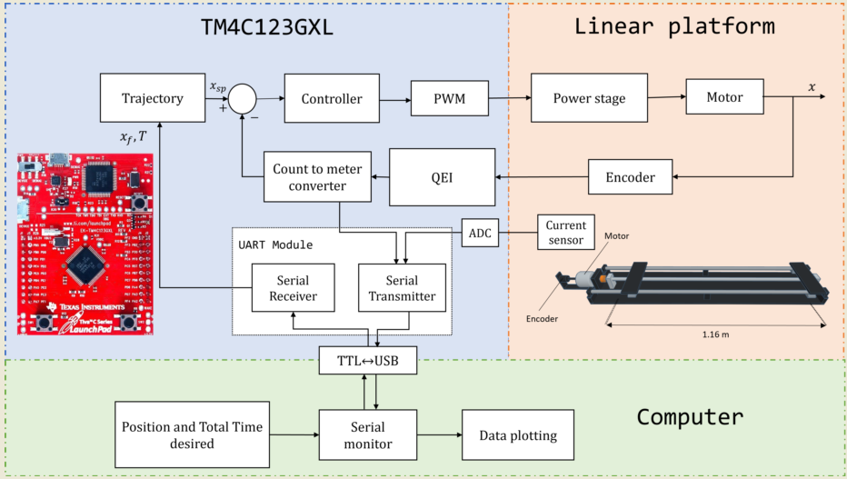
This section describes the implementation of the motion control system that has been made. In this system, a classic PID controller and a motion profile generator have been integrated into a microcontroller to control the position of the carriage of a linear platform. To allow configuration and adjustment of the motion profile parameters, serial communication is established between the microcontroller and a computer. Figure 7 shows the general diagram of the blocks that comprise the proposed system.
The first block consists of the plant described in the last section. The second block is the embedded system. In this stage, the microcontroller schedules sensing tasks for measuring both the current and the position of the encoder, which allows for obtaining information on the state of the motor. In addition, the microcontroller computes the motion profile using the received data to determine the carriage’s speed, acceleration, and displacement. Once the motion profile has been calculated, PID controller adjusts the trajectory using the position information. The control signal is applied to the motor driver, the HW-039 BTS7960, via a Pulse-Width-Modulation (PWM) signal.
The third component of the system is a computer, which is linked to the ARM microcontroller using the PL2303HX TTL-USB converter. During the tests, the computer sends data to the embedded system regarding the required displacement and the total time for the execution of the movement. These data define the parameters of the movement profile and the duration of the operation. On the other hand, the microcontroller sends data to the computer about the current position of the motor, the computed control signal, and the current consumed by the motor. These data allow real-time monitoring and visualization of the status and performance of the control system.
The direct manipulation of the microcontroller registers provides greater control and optimization of the system, adapting it to the specific needs of this project, one of which is the sampling time of the entire proposed system. The flowchart in Figure 8 shows the algorithm used to program the embedded system.
4.3. Initial definitions of the microcontroller memory addresses
In the initial stage of the programming process, the memory addresses of the registers related to the device’s configuration are defined. These registers are essential to establish and control the behavior of the different components of the microcontroller. In addition to memory addresses, global variables, and constant values are established. Global variables can be accessed and used anywhere in the program, making exchanging information between code sections easy. On the other hand, constant values are those that do not change throughout the execution of the program and are used to establish parameters or static configurations.
4.4. Initial configuration
In this subsection, the configuration of the necessary registers for the correct operation of the microcontroller is carried out. By default, the microcontroller operates at a frequency of 16 MHz, but by appropriately modifying the corresponding registers, it is possible to reach a maximum operating frequency of 80 MHz. Once the operating frequency has been configured, proceed to the activation and configuration of input/output ports. These ports allow communication and connection with other external devices, facilitating the interaction of the microcontroller with its environment. In addition to the input/output ports, other necessary peripheral modules must be initialized. For example, the Quadrature Encoder Interface (QEI) module is configured to allow quadrature reading of the encoder, which provides greater accuracy in motor position measurement. In addition, the PWM module is configured to generate two PWM signals at a frequency of 5 kHz, allowing efficient control of the speed and power supplied to the motor. In the same way, the initialization of the ADC module is performed, which enables the conversion of analog signals to digital for further processing. On the other hand, the Universal Asynchronous Receivers/Transmitter (UART) module is configured to operate at a speed of 115200 baud, which facilitates serial communication with other devices. The last module to configure is the Systick Timer. This 24-bit timer is loaded with RELOAD_VALUE, a value given by the Equation (36) to generate an interrupt every t seconds, which allows ensuring a time-fixed sampling. However, before starting the timer count, and T are set according to the information received by serial communication.
Within the program’s main loop, a series of tasks are carried out periodically every , corresponding to the system sampling time. First, the trajectory calculation is performed, which involves determining the desired position or the path that the system should follow. Next, the current is measured, an important parameter to evaluate the performance and load of the motor. This measurement is carried out through an ACS712 model current sensor. Subsequently, the control algorithm is executed, which uses the trajectory information to generate the appropriate control signal. The control algorithm is based on a discrete PID controller. Finally, the measured data is sent to the computer using the UART module.
4.5. Implementation of motion profiles
For the implementation of the velocity profiles, in each iteration, k, a point of the trajectory, is calculated for the current time instant . In the case of the parabolic profile, the trajectory is calculated in the microcontroller with Equation (37), which is a simplification of Equation (4) in which is considered and .
Regarding the trapezoidal profile, Equation (10) is reduced to Equation (38) considering the initial position and time equal to 0.
The s-curve velocity profile is calculated with the Equations (39), (40) and (41), obtained after the discretization of the Equations (21), (22) and (23) by Euler’s method backward.
Where k is the sample number, whereas , , and are the current jerk, acceleration, velocity and position, respectively.
4.6. Implementation of the control algorithm
The control algorithm starts with the encoder reading. The value is converted to meters by multiplying the count by . The error is calculated as the deviation between the position in meters and the actual set point given by the trajectory generator. The control signal is generated with Equations (43) and (42), obtained from the discretization of the PID controller by Euler’s backward method.
The value obtained by the control signal represents a voltage in the V range, which is the DC motor’s operating range. The control signal is scaled to the microcontroller’s operating range V by modifying the duty cycle of the PWM signal, given by Equation (44).
Where PWM_LOAD is the value to load to the configuration register to generate a 5 kHz PWM signal, is the maximum voltage (in this case 24 V), is the control signal and PWM_CMP is the value to load in the register that modifies the duty cycle.
4.7. Timer ended
After sending the measurements to the computer, wait for the timer to expire. To do this, the account status indicator is checked. When it reaches zero, the counter resets, and the loop starts again.
5. Experimental Results
This section presents the results obtained by applying the three velocity profiles to the position controller. Figure 9 shows the linear plant used for the experimentation. This figure details the main elements that make up the motion control system.
5.1. Parabolic profile without load
The carriage of the plant is moved at a distance of m in 4 seconds. Two cases are considered for each profile: the first without a load on the carriage and the second with a load of 9 kg. Table 1 summarizes the parameters used for implementing the parabolic velocity profile.
Figure 10(a) compares the carriage position obtained experimentally versus the ideal trajectory of the velocity profile. In both graphs, the final position of the carriage corresponds to the target position in the required time T. In addition, the graph of the percentage error in Figure 10(b) shows a higher performance of the controller in terms of tracking trajectory as tends towards zero for most of the execution time of the movement. is obtained with Equation (46), where is the actual position and is the reference position calculated with the profile.
The speed is calculated offline using central difference approximation given by Equation (47) for the first derivative of the experimental position.
Figure 10(c) shows the estimated speed after applying a low-pass filter of the FIR type. The resulting graph’s shape is close to that of the implemented velocity profile; the estimated maximum velocity of agrees with the calculated maximum velocity. On the other hand, the acceleration is obtained with the same numerical method of Equation (47). The acceleration computed and that of the profile are compared in Figure 10(d), in which is notorious the abrupt change in acceleration that the velocity profile presents at the beginning and end of the movement.
The control signal applied to the system is depicted in Figure 11(a). A maximum voltage of 9.8 V is observed for the no-load case. It is important to note that the shape of the control signal closely follows the speed modeled by the profile. Figure 11(b) shows the current consumed during the execution of the movement. The maximum current value obtained was 1.12 A. Figure 11(c) shows the instantaneous power. The energy, calculated from the integration of the instantaneous power, is shown in Figure 11(d). The total energy consumed was 23.7044 J.
5.2. Trapezoidal profile without load
Regarding the trapezoidal velocity profile, Table 2 shows the parameters used to match the same displacement and execution time as the parabolic profile. The calculated maximum velocity of is the same as in the trapezoidal velocity profile. However, the maximum acceleration is reduced from to .
Figure 12(a) presents a comparison between the experimental and ideal position of the profile. It can be seen, in Figure 12(b), that the error drops to less than in s. On the other hand, Figure 12(c) shows that the estimated velocity is numerically close to that determined by the profile. Figure 12(d) offers the estimated acceleration; four abrupt changes are observed: The first occurs at the beginning of the acceleration phase at , where the acceleration rises from 0 to . The second one happens at the beginning of the constant velocity phase at , where the acceleration drops to 0. The third abrupt change in acceleration rises from 0 to at , where the deceleration phase starts. The last one is presented at the end of the movement at . The acceleration suddenly changes from to 0.
From Figure 13(a), it can be seen that at the beginning of the constant speed phase in , the control signal presents a maximum peak voltage of V, caused by the abrupt change in the acceleration is subsequently maintained at V until the beginning of the deceleration phase at , where it begins to drop to zero.
The current presents a similar behavior. Figure 13(b) shows that in , a maximum current of 1.43 A is measured. During the constant speed phase, the current consumed is 1.04 A. Since instantaneous power is calculated as the product of voltage times current, the power graph in Figure 13(c) shows its maximum value at . According to Figure 13(d), the total energy consumed is 25.964 J.
5.3. S-curve profile without load
Table 3 presents the selected and calculated parameters for generating the S-curve velocity profile. The maximum velocity obtained from is the largest of the three profiles. In contrast, the maximum acceleration of is more significant than in the trapezoidal but less than in the parabolic profile.
Figure 14(b) shows an approximation of the position of the carriage to that of the calculated profile, which due to numerical integration has a % with regard to the final position. However, a reduction of the following error to less than in 0.8 seconds is presented in Figure 14(b). Similarly, in Figure 14(c), the maximum velocity of , is close to 0.333 of the profile of speed. Regarding the acceleration graphs of Figure 14(d), the acceleration measured does not exhibit the abrupt changes observed in the two previous profiles.
The control signal generated for the S-curve velocity profile in Figure 15(a) has a maximum voltage of 11 V. This is the profile with the highest maximum voltage in the control signal and the one that reaches the highest speed during the execution of the movement. As for the current shown in Figure 15(b), the maximum peak presented was A, which gradually reduced to A during the constant velocity phase. The power and energy graphs are shown in the Figure 15(c) and Figure 15(d), respectively. The total energy consumed is 26.952 J.
5.4. Experimentation with load
This section reports the experimental results adding a load of 9 Kg on the carriage. First, the tracking error for each profile is compared in Figure 16. In this figure, it can be noted the robustness of the controller since despite adding a load to the system, the carriage maintains the position for each profile under test.
The control signal computed for each of the three profiles when a load is placed on the carriage is presented in Figure 17. In the case of the parabolic profile, the control signal reaches a maximum value of 9.8 V. For the trapezoidal profile, a maximum voltage of 11 V is presented at t= due to the discontinuity in acceleration. The voltage delivered is 9.6 V in the constant speed phase. The S-curve profile shows the values of voltage maximums, 11.2 V in the acceleration phase and 10.2 V in the constant speed phase. By comparing these values with those of the no-load case, we observed that the control signal of the loaded case presented higher voltage values than the no-load case.
Figure 18 shows the current consumption of the three implemented velocity profiles. The graph of the current corresponding to the parabolic profile shows that the maximum current is 1.11 A. While for the trapezoidal velocity profile, the maximum current is 1.58 A. Finally, using the S-curve type trajectory, a maximum current of 1.77 A has the highest current amplitude of the three profiles.
The instantaneous power of the three profiles is depicted in Figure 19. It is observed again that the S-curve velocity profile gives the highest dissipated power, while the parabolic profile is the lowest since the latter presented lower voltage and current consumption than the other two profiles.
Finally, Figure 20 displays the energy consumption of the three motion profiles. From the graph, it can be seen that the profile with the highest energy consumption is the S-curve with J, followed by the trapezoidal speed profile with J and the parabolic with J, the latter being the one with the lowest consumption of the three profiles implemented.
The Table 4 presents a comparative chart of the total energy consumed in each profile when no load was placed on the carriage and when it was used. In both circumstances 40 tests for each profile were carried out, and as can be seen, the energy consumption is higher in the S-curve profile and lower in the parabolic velocity profile.
6. Conclusions
This paper presented a methodology that allows designing and implementing open architecture motion controllers, from selecting the embedded system to implementing it in a linear platform composed of a direct current motor coupled to an endless screw to measure the energy consumption of trajectories. The control algorithm is based on a classic PID controller whose reference signal is given by a motion profile generator. The selected embedded system allowed a sampling time of 0.001 s, with which an adequate system response for controlling direct current motors is obtained. The motion profiles used in this work were of the polynomial type: trapezoidal, parabolic, and S-curve. The same displacement length h was considered for calculating each of the trajectories and the exact total movement time T. The kinematic magnitudes of the three profiles, such as position, velocity, and acceleration, were compared during the experimentation. The S-curve profile presented the most significant magnitude in speed, and the parabolic profile had the highest acceleration. However, the main characteristic analyzed was the energy consumption, which required analyzing the control signal, the measured current, and the instantaneous power to be estimated using numerical integration techniques. The results showed that the parabolic speed profile presented the lowest amplitude in the control signal, current, and power. In contrast, the S-curve speed profile was the one that presented the highest amplitude in the same magnitudes mentioned. Table 4 shows that the highest energy consumption was dissipated using the S-curve profile, while the parabolic trajectory consumed less than the other two. In fact, after carrying out 40 tests for each profile, the energy consumption in the parabolic profile was % less than the trapezoidal profile and % less than the s-curve profile. In a second case, the same analysis was carried out, placing a load of 9 on the carriage; the robustness of the controller allowed for obtaining similar results in position, velocity, and acceleration for each profile compared to the case with no load. The difference identified was in the control signal and current consumed, translating into higher energy consumption. Nevertheless, from Table 4, it is clear that the parabolic velocity profile also had the lowest energy consumption despite adding the load. Based on the results, trajectory planning is an effective technique easy to implement in low-cost microcontrollers to reduce energy consumption in motion control systems. In future studies, the S-curve parameters will be modified to reduce the maximum velocity and analyze the energy consumption behavior. Finally, a fuzzy controller will be used so as not to require the mathematical model of the plant.
Author Contributions
Conceptualization, L.F.O-G and J.R.G-M; methodology, L.F.O-G; software, L.F.O-G and E.E.C-M; validation, L.F.O-G, J.R.G-M and E.E.C-M.; formal analysis, J.R.G-M; investigation, L.F.-G and O.A.B-V; resources, J.R.G-M, E.E.-C, O.A.B-V, M.G-L and T.M-S; data curation, M.G-L and T.M-S; writing—original draft preparation, J.R.G-M, M.G-L and T.M-S; writing—review and editing, J.R.G-M; visualization, M.G-L and T.M-S; supervision, J.R.G-M; project administration, J.R.G-M and L.F.O-G.
Funding
CONAHCYT funded this research under the scholarship 1271936.
Institutional Review Board Statement
Not applicable.
Informed Consent Statement
Not applicable.
Acknowledgments
This work was carried out thanks to the support of the Faculty of Mechanical and Electrical Engineering and the Faculty of Electronic and Communications Engineering, Poza Rica, Ver., Mexico.
Conflicts of Interest
The authors declare no conflict of interest.
Abbreviations
The following abbreviations are used in this manuscript:
| PID | Proportional-Integral-Derivative |
| DC | Direct Current |
| ARM | Advanced RISC Machine |
| ADC | Analog-to-Digital converter |
| PWM | Pulse Width Modulation |
| GPIO | Genaral-Purpose Input/Output |
| GPTM | Genral-Purpose Timer |
| UART | Universal Asynchronous Receivers/Transmitter |
| QEI | Quadrature Encoder Interface |
| PPR | Pulses per revolution |
Appendix A

Table A1.
Main features of the TM4C123GH6PM microcontroller.
| Feature | Description |
|---|---|
| Core | ARM Cortex-M4F |
| Performance | 80-MHz operation |
| Universal Asynchronous Receivers/ Transmitter (UART) |
8 Modules |
| General-Purpose Timer (GPTM) | 6-16/32-bit GPTM blocks and six 32/64-bit Wide GPTM blocks |
| General-Purpose Input/Output (GPIO) | 6 physical GPIO blocks |
| Pulse Width Modulator | 2 PWM modules, each with four PWM generator blocks and a control block, for a total of 16 PWM outputs. |
| Quadrature Encoder Interface (QEI) | 2 QEI modules |
| Analog-to-Digital Converter (ADC) | 2-12-bit ADC modules, with a maximum sample rate of one million samples/second |
References
- Wu, Z.; Chen, J.; Bao, T.; Wang, J.; Zhang, L.; Xu, F. A Novel Point-to-Point Trajectory Planning Algorithm for Industrial Robots Based on a Locally Asymmetrical Jerk Motion Profile. Processes 2022, 10, 728. [Google Scholar] [CrossRef]
- Carabin, G.; Scalera, L. On the trajectory planning for energy efficiency in industrial robotic systems. Robotics 2020, 9, 89. [Google Scholar] [CrossRef]
- Boryga, M.; Kołodziej, P.; Gołacki, K. The Use of Asymmetric Polynomial Profiles for Planning a Smooth Trajectory. Appl. Sci. 2022, 12, 12284. [Google Scholar] [CrossRef]
- Wu, G.; Zhang, S. Real-time jerk-minimization trajectory planning of robotic arm based on polynomial curve optimization. Proc IMechE Part C: J Mechanical Engineering Science 2022, 0, 1–13. [Google Scholar] [CrossRef]
- Sang, W.; Sun, N.; Zhang, C.; Qiu, Z.; Fang, Y. Hybrid Time-Energy Optimal Trajectory Planning for Robot Manipulators With Path and Uniform Velocity Constraints. In Proceedings of the 2022 13th Asian Control Conference (ASCC), Jeju, Republic of Korea, 4-7 May 2022; pp. 334–340. [Google Scholar]
- Kröger, T. On-Line Trajectory Generation in Robotic Systems: Basic Concepts for Instantaneous Reactions to Unforeseen (Sensor) Events, 1st ed.Springer, 2010; pp. 11–29. [Google Scholar]
- Martínez, J.R.G.; Reséndiz, J.R.; Prado, M.Á.M.; Miguel, E.E.C. Assessment of jerk performance s-curve and trapezoidal velocity profiles. In Proceedings of the 2017 XIII International Engineering Congress (CONIIN), Santiago de Queretaro, Mexico, 15–19 May 2017; pp. 1–7. [Google Scholar]
- Ha, C. W.; Lee, D. Analysis of Embedded Pre-filters in Motion Profiles. IEEE Transactions on Industrial Electronics 2017, 65, pp–1481. [Google Scholar]
- Mejerbi, M; Knani, J. Influence of the motion profile on the performance of a flexible arm. In Proceedings of the 2017 International Conference on Control, Automation and Diagnosis (ICCAD), Hammamet, Tunisia, 19-21 January 2017; pp. 76–81.
- Alpers, B. On Fast Jerk-Continuous Motion Functions with Higher-Order Kinematic Restrictions for Online Trajectory Generation. Robotics 2022, 11, 73. [Google Scholar] [CrossRef]
- Nguyen, K. D.; Chen, I. M.; Ng, T. C; Planning algorithms for s-curve trajectories. In Proceedings of the 2007 IEEE/ASME international conference on advanced intelligent mechatronics, Zurich, Switzerland, 4-7 September 2007; pp. 1–6. [Google Scholar]
- Lee, D.; Ha, C. W. Optimization process for polynomial motion profiles to achieve fast movement with low vibration. IEEE Transactions on Control Systems Technology 2020, 28, 1892–1901. [Google Scholar] [CrossRef]
- Nam, N. Q. Characteristics of S-curve motion profile for all ranges of motion length and limits. In Proceedings of the 2020 International Conference on Advanced Mechatronic Systems (ICAMechS), Hanoi, Vietnam, 10-13 December 2020; pp. 214–220. [Google Scholar]
- Rubio F; Llopis-Albert C; Valero F; Suñer JL. Industrial robot efficient trajectory generation without collision through the evolution of the optimal trajectory. Robotics and Autonomous Systems 2016, 86, 106–112. [Google Scholar]
- Van Oosterwyck, N.; Vanbecelaere, F.; Knaepkens, F.; Monte, M.; Stockman, K.; Cuyt, A.; Derammelaere, S. Energy Optimal Point-to-Point Motion Profile Optimization Mechanics Based Design of Structures and Machines 2022, 1–18.
- Chamraz, Š. and Balogh, R. In Optimal structure for the trajectory controller. In Proceedings of the 2016 Cybernetics & Informatics (K&I), Levoca, Slovakia, 2-5 February 2016; pp. 1–5. [Google Scholar]
- Al-khayyt, SZ. Comparison between fuzzy logic based controllers for robot manipulator trajectory tracking. In Proceedings of the 2012 First National Conference for Engineering Sciences (FNCES), Baghdad, Iraq, 7-8 November 2012; pp. 1-6. [Google Scholar]
- Lin, CY. Neural network adaptive control and repetitive control for high performance precision motion control. In Proceedings of the SICE Annual Conference 2010, Taipei, Taiwan, 18-21 August 2010; pp. 2843–2844. [Google Scholar]
- Biagiotti, L.; Melchiorri, C. Optimization of generalized S-curve trajectories for residual vibration suppression and compliance with kinematic bounds. IEEE/ASME Transactions on Mechatronics 2020, 26, 2724–2734. [Google Scholar] [CrossRef]
- Lee, D.; Ha, C. W. Optimization process for polynomial motion profiles to achieve fast movement with low vibration. IEEE Transactions on Control Systems Technology 2020, 28, 1892–1901. [Google Scholar] [CrossRef]
- Rymansaib, Z.; Iravani, P.; Sahinkaya, M. N. Exponential trajectory generation for point to point motions. In Proceedings of the 2013 IEEE/ASME international conference on advanced intelligent mechatronics, Wollongong, NSW, Australia, 9-12 July 2013; pp. 906–911. [Google Scholar]
- Scalera, L.; Carabin, G.; Vidoni, R.; Gasparetto, A. Minimum-energy trajectory planning for industrial robotic applications: analytical model and experimental results. In Advances in Service and Industrial Robotics: Results of RAAD; Zeghloul, S., Laribi, M. A., Arevalo, J. S. S, Eds.; Springer International Publishing: Cham, Switzerland, 2020; pp. 334–342. [Google Scholar]
- Gasparetto, A.; Boscariol, P.; Lanzutti, A.; Vidoni, R. Path planning and trajectory planning algorithms: A general overview. In Motion and Operation Planning of Robotic Systems: Background and Practical Approaches; Carbone, G., Gomez-Bravo, F., Eds.; Springer International Publishing: Switzerland, 2015; pp. 3–27. [Google Scholar]
- Fang, Y; Hu J; Liu, W; Shao, Q; Qi, J; Peng, Y. Smooth and time-optimal S-curve trajectory planning for automated robots and machines. Mechanism and Machine Theory 2019, 137, 127–153. [Google Scholar] [CrossRef]
- Alpers, B. On Fast Jerk–, Acceleration– and Velocity–Restricted Motion Functions for Online Trajectory Generation. Robotics 2021, 10, 25. [Google Scholar] [CrossRef]
- Wang, H; Wang, H; Huang, J; Zhao, B; Quan, L. Smooth point-to-point trajectory planning for industrial robots with kinematical constraints based on high-order polynomial curve. Mechanism and Machine Theory 2019, 139, 284–293. [Google Scholar] [CrossRef]
- Carabin, G.; Wehrle, E.; Vidoni, R. A Review on Energy-Saving Optimization Methods for Robotic and Automatic Systems. Robotics 2017, 6, 39. [Google Scholar] [CrossRef]
- Assad, F.; Rushforth, E.; Ahmad, B.; Harrison, R. (2018, August). An Approach of Optimising S-curve Trajectory for a Better Energy Consumption. In proceedings of the 2018 IEEE 14th International Conference on Automation Science and Engineering (CASE), Munich, Germany, 20-24 August 2018; pp. 98–103. [Google Scholar]
- Montalvo, V.; Estévez-Bén, A.A.; Rodríguez-Reséndiz, J.; Macias-Bobadilla, G.; Mendiola-Santíbañez, J.D.; Camarillo-Gómez, K.A. FPGA-Based Architecture for Sensing Power Consumption on Parabolic and Trapezoidal Motion Profiles. Electronics 2020, 9, 1301. [Google Scholar] [CrossRef]
- Carabin, G.; Vidoni, R. Energy-saving optimization method for point-to-point trajectories planned via standard primitives in 1-DoF mechatronic systems. Int J Adv Manuf Technol 2021, 116, 331–344. [Google Scholar] [CrossRef]
- Hosseini, S; Hahn, I. Energy-efficient motion planning for electrical drives. In Proceedings of the 2018 IEEE Electrical Power and Energy Conference (EPEC), Toronto, Canada, 10-11 Octuber 2018; pp. 1–7.
- Nshama, EW, Msukwa, MR, Uchiyama N. A trade-off between energy saving and cycle time reduction by Pareto optimal corner smoothing in industrial feed drive systems. IEEE Access 2021, 9, 23579–23594. [Google Scholar] [CrossRef]
- Halinga, M. S.; Nyobuya, H. J.; Uchiyama, N. Generation of Time and Energy Optimal Coverage Motion for Industrial Machines Using a Modified S-Curve Trajectory. In Proceedings of the 2023 IEEE/SICE International Symposium on System Integration (SII), Atlanta, GA, USA, 17-20 January 2023; pp. 1–6. [Google Scholar]
- Biagiotti, L.; Melchiorri, C. Trajectory planning for automatic machines and robots, 1st ed.; Springer: Berlin/Heidelberg, Germany, 2008; pp. 1–13. [Google Scholar]
- Ali, S. A.; Annuar, K. A. M.; Miskon, M. F. Trajectory planning for exoskeleton robot by using cubic and quintic polynomial equation. International Journal of Applied Engineering Research 2016, 11, 7943–7946. [Google Scholar]
- Moritz, F. G. Electromechanical motion systems: Design and simulation, 1st ed.; John Wiley & Sons: West Sussex, United Kingdom, 2014; pp. 167–194. [Google Scholar]
- Heo, H.-J.; Son, Y.; Kim, J.-M. A Trapezoidal Velocity Profile Generator for Position Control Using a Feedback Strategy. Energies 2019, 12, 1222. [Google Scholar] [CrossRef]
- García-Martínez, J. R.; Cruz-Miguel, E. E; Carrillo-Serrano, R. V.; Mendoza-Mondragón, F.; Toledano-Ayala, M.; Rodríguez-Reséndiz, J. A PID-type fuzzy logic controller-based approach for motion control applications. Sensors 2020, 20, 5323. [Google Scholar] [CrossRef] [PubMed]
Figure 1.
Parabolic velocity profile (a) Position, (b) Velocity and (c) Acceleration.
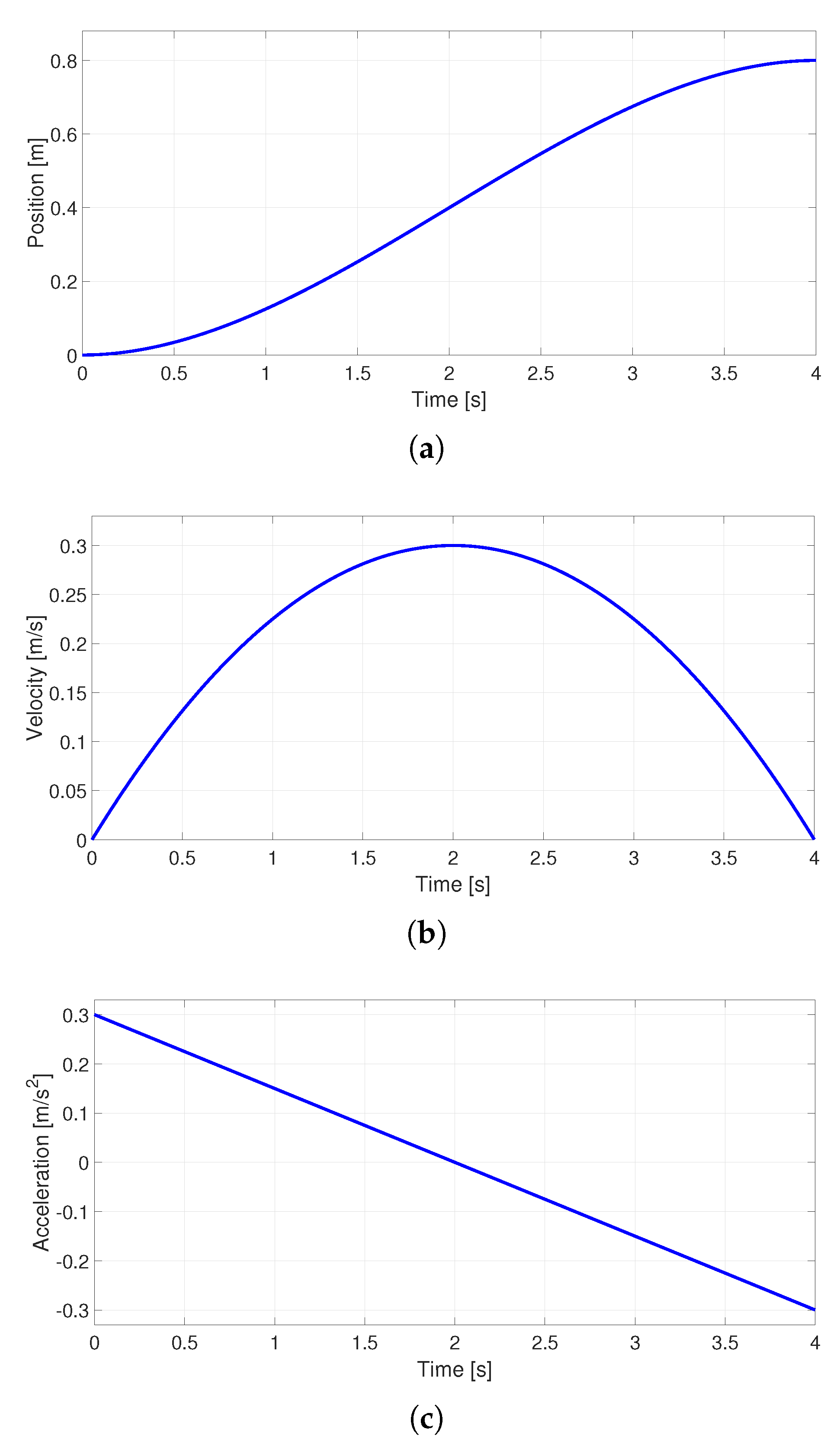
Figure 2.
Trapezoidal velocity profile (a) Position, (b) Velocity and (c) Acceleration.
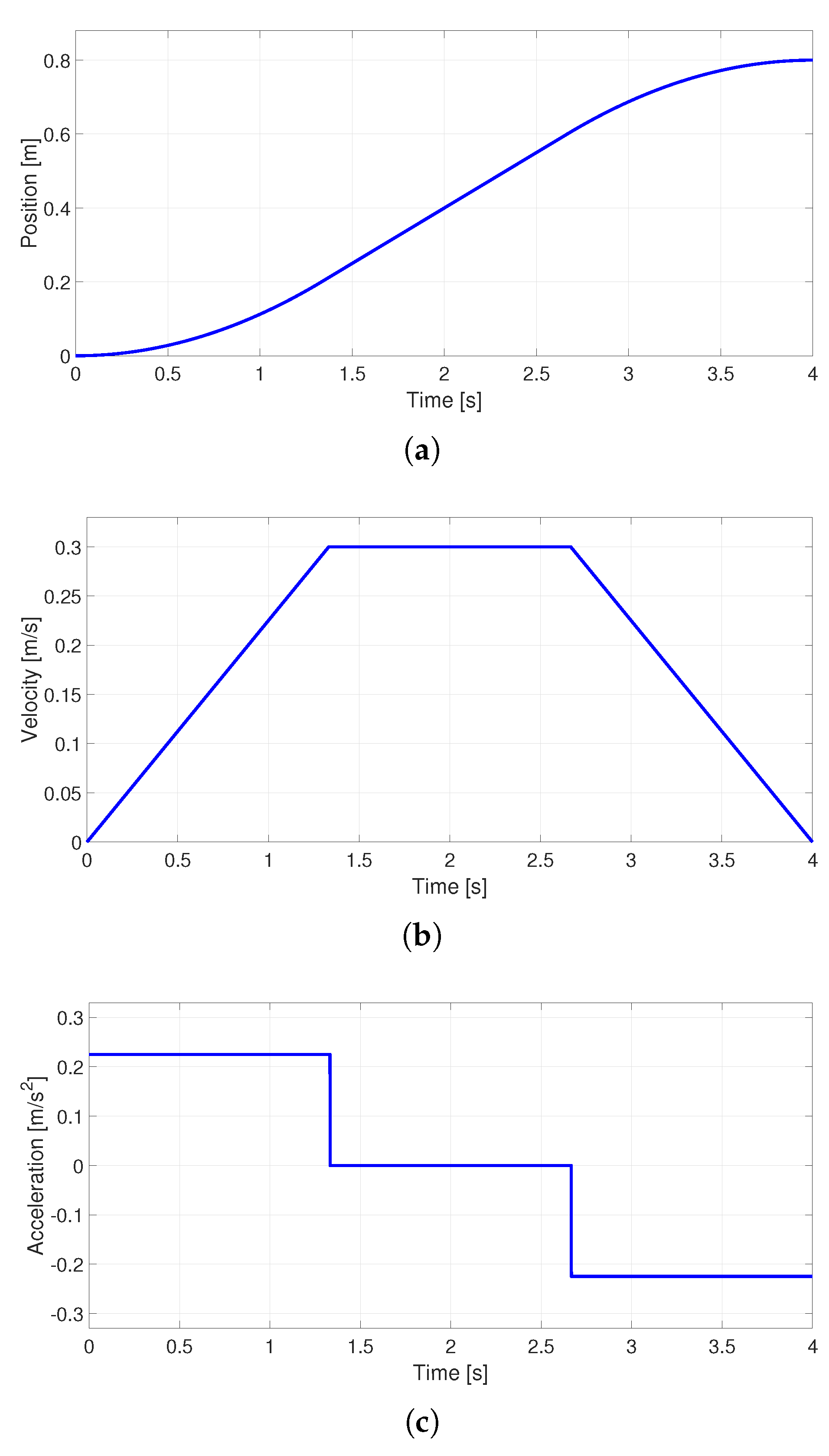
Figure 3.
S-curve velocity profile (a) Position, (b) Velocity, (c) Acceleration and (d) Jerk.
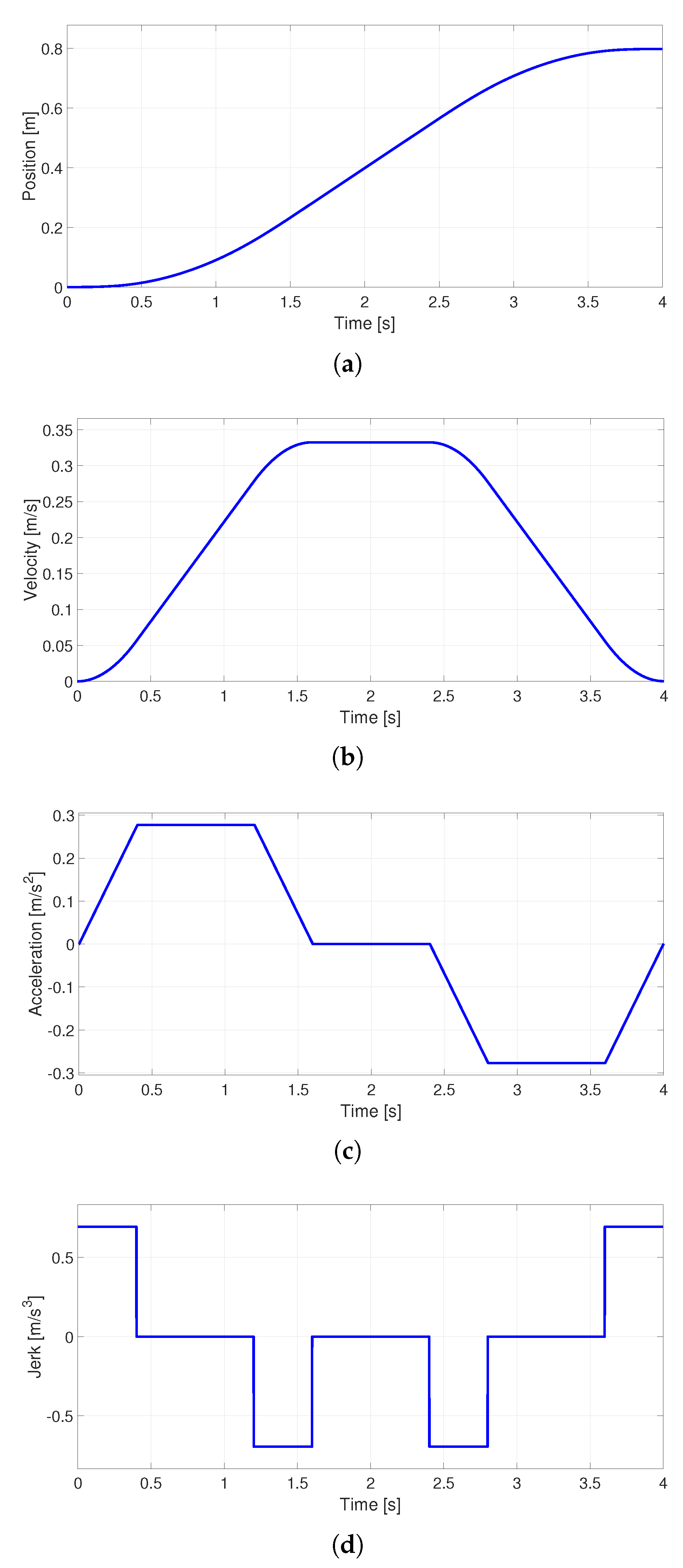
Figure 4.
Design stages of a motion controller.
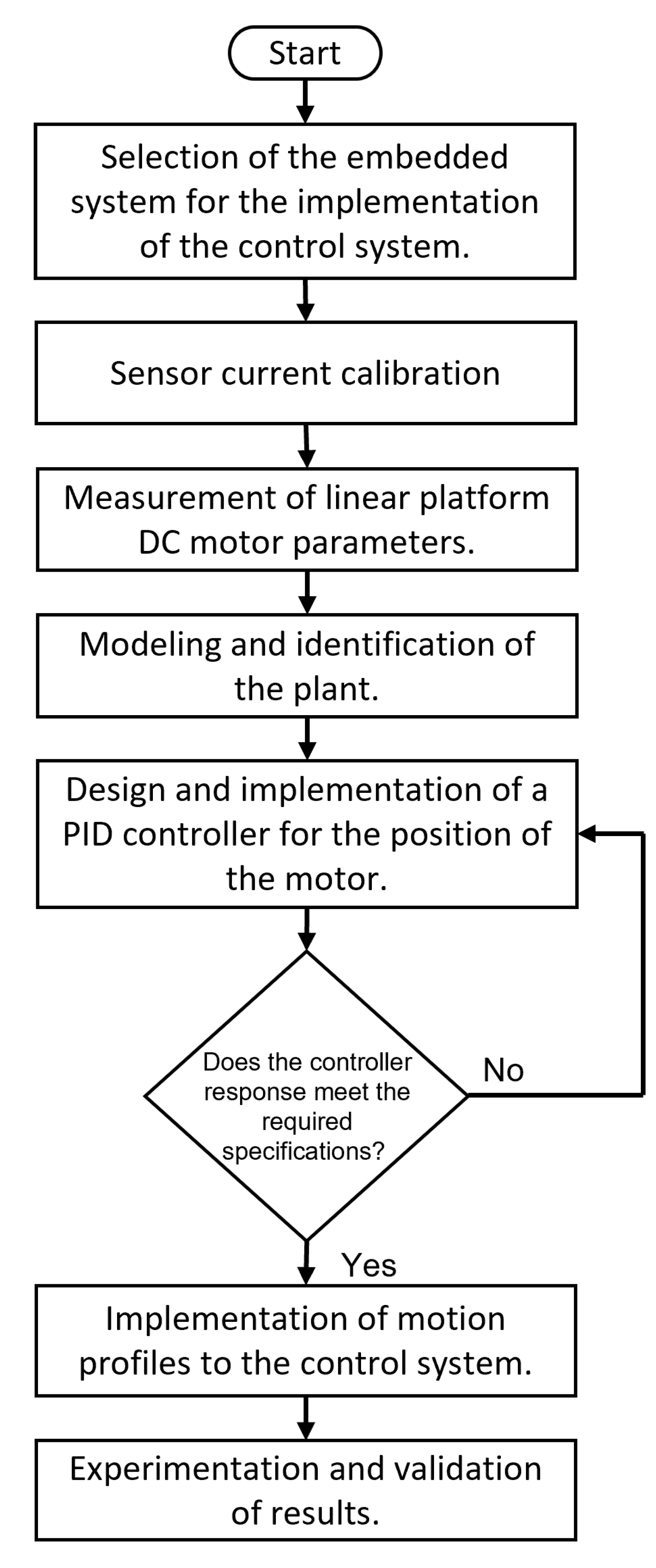
Figure 5.
Block diagram of the system used for identification.
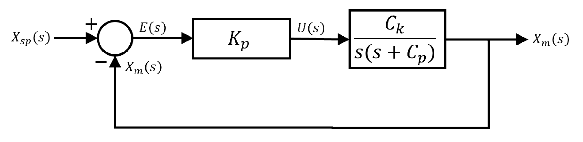
Figure 6.
PID algorithm structure.
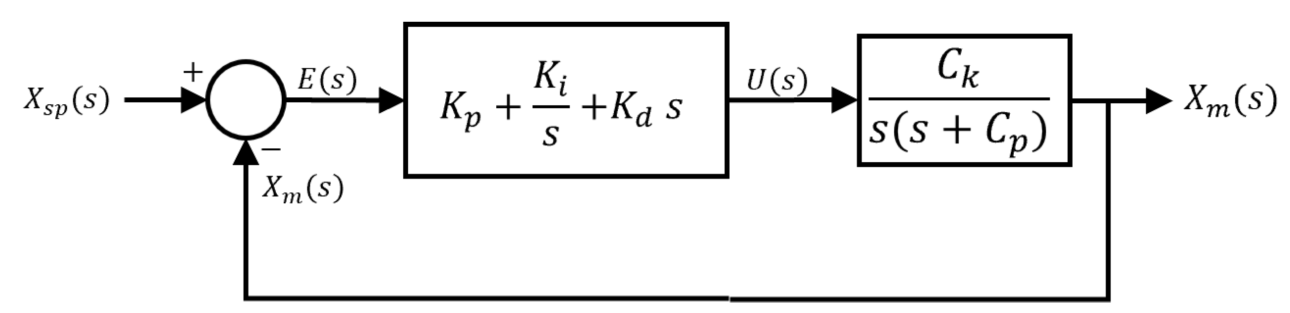
Figure 7.
Approach of the entire system implementation.
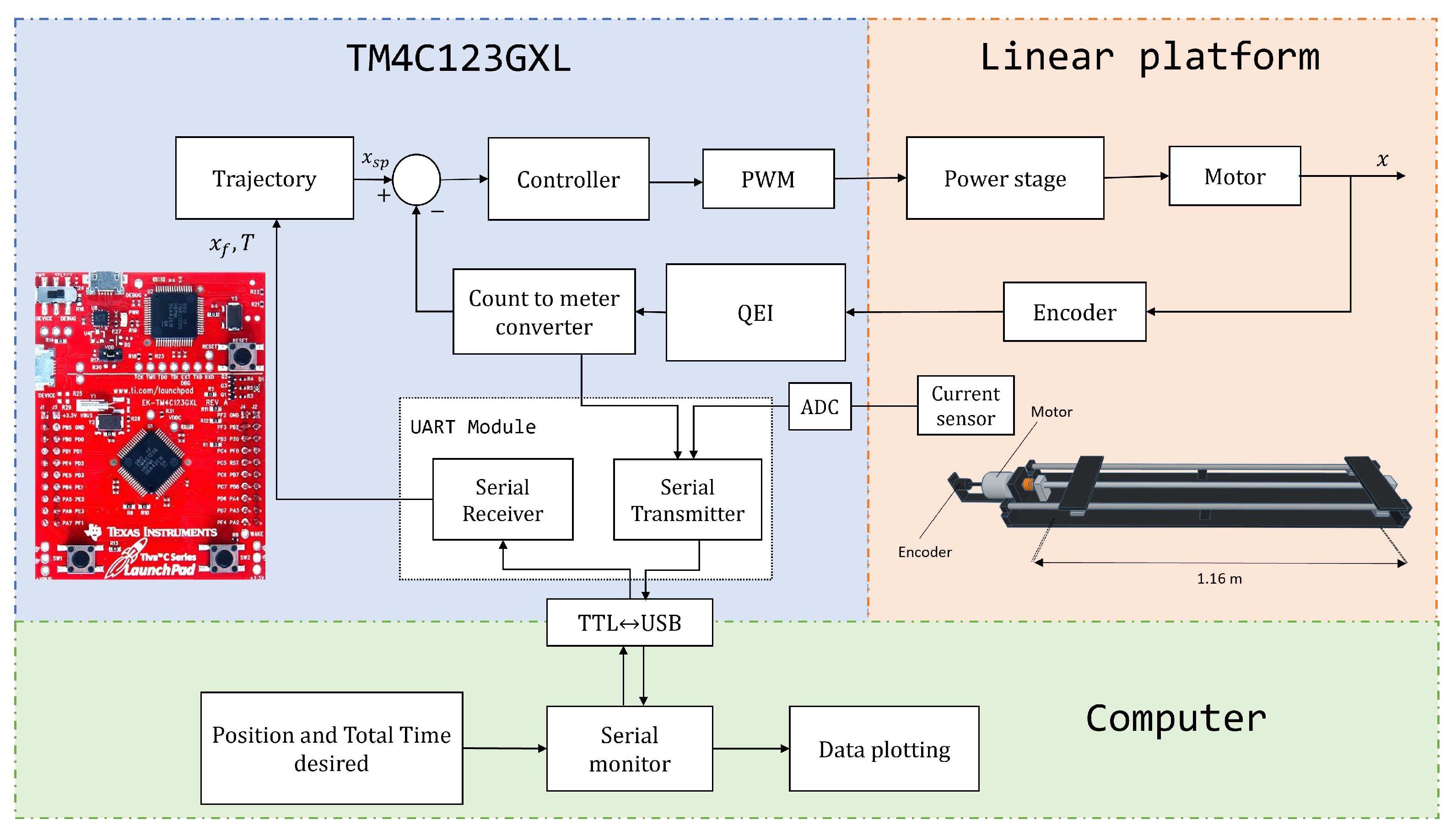
Figure 8.
Flowchart of the algorithm used for the microntroller programming.
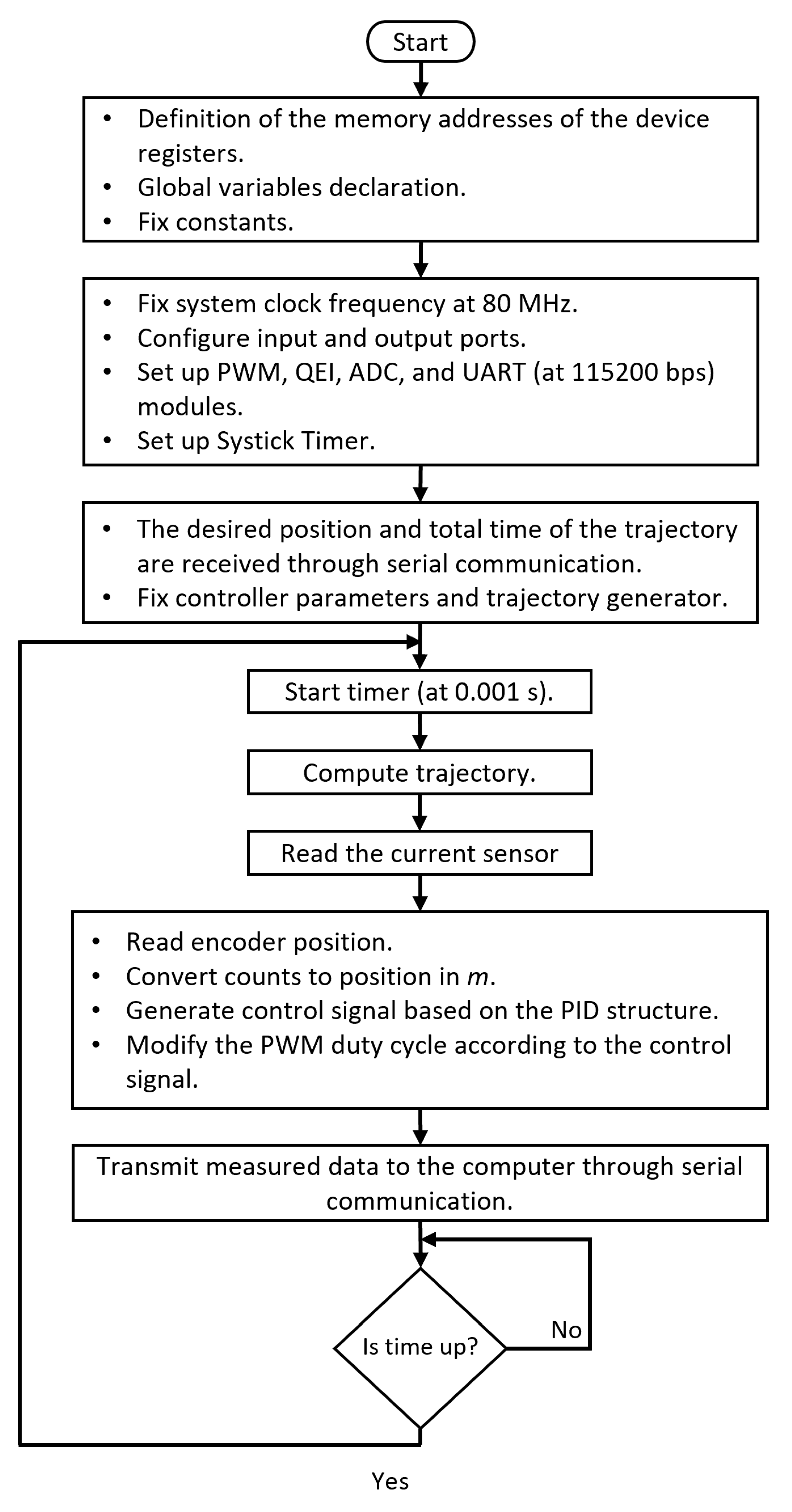
Figure 9.
Linear plant used for the experimentation.
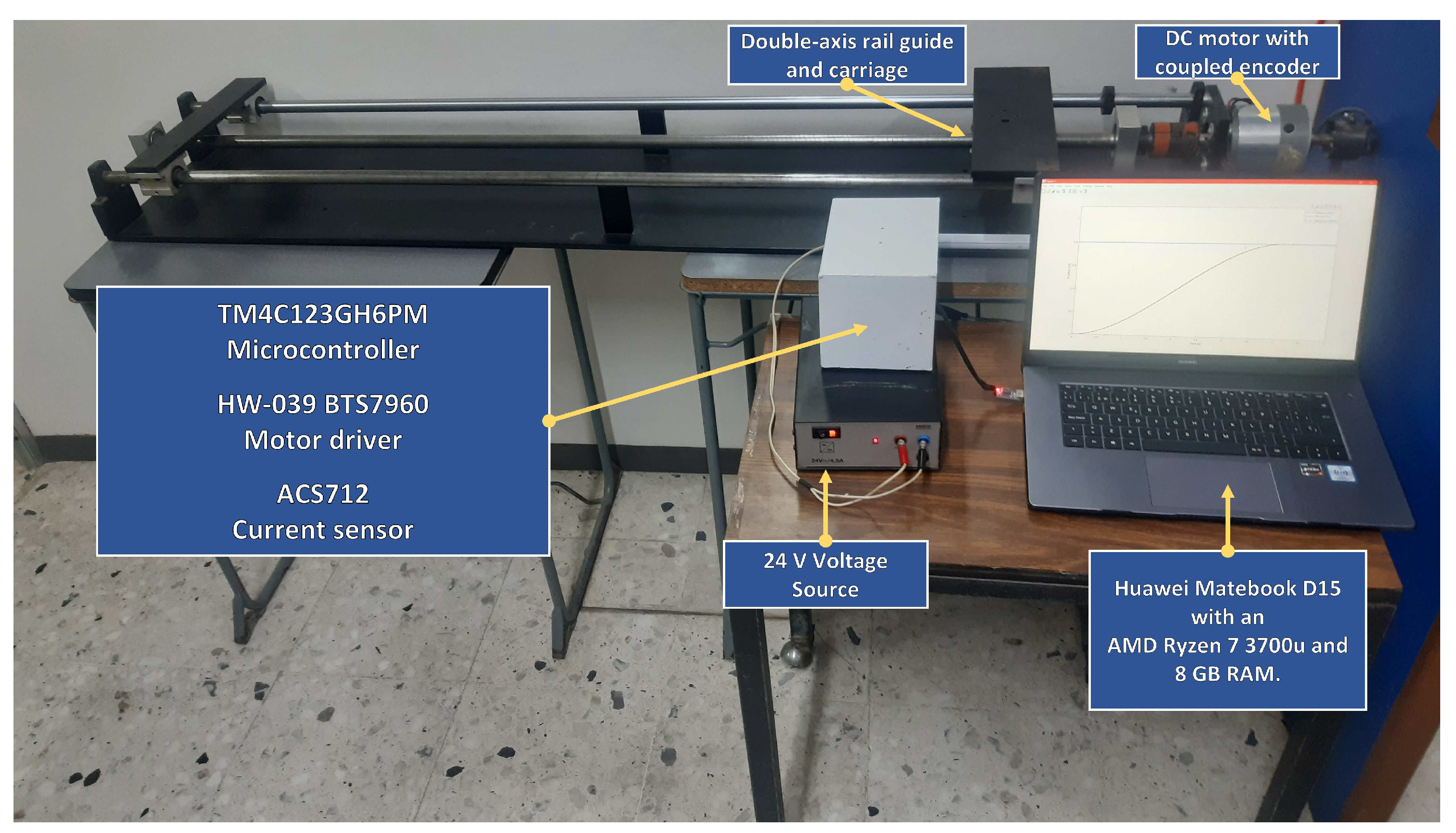
Figure 10.
Parabolic velocity profile (a) Position, (b) Error (c) Velocity and (d) Acceleration.
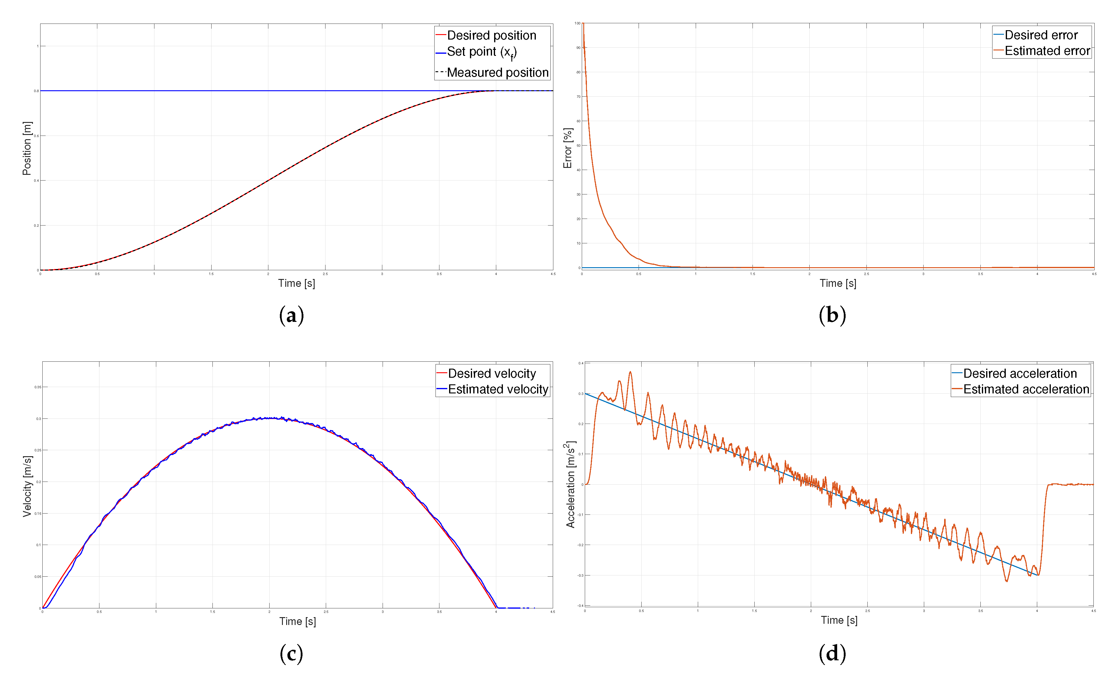
Figure 11.
Parabolic velocity profile (a) Control signal, (b) Current (c) Power and (d) Energy.
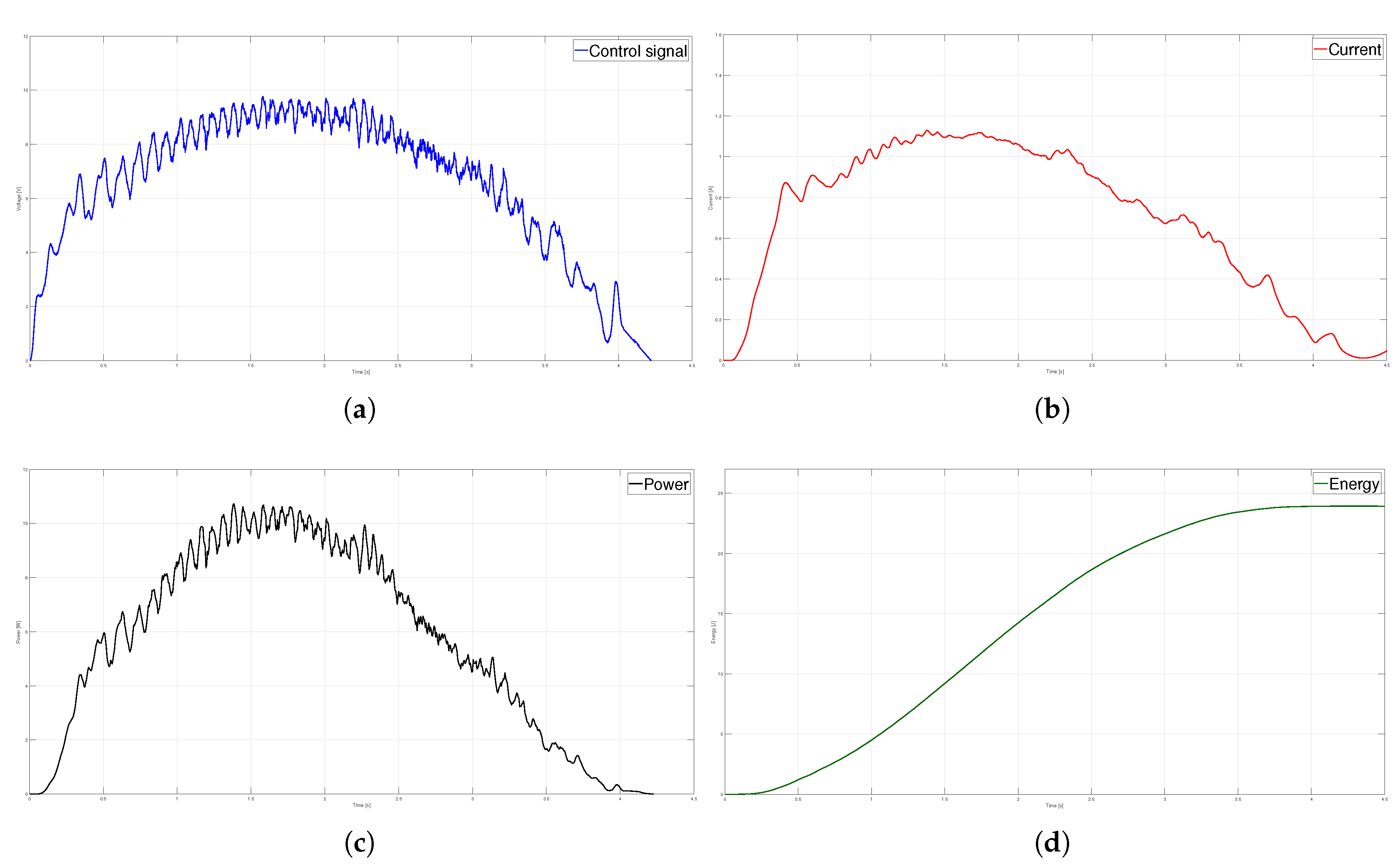
Figure 12.
Trapezoidal velocity profile (a) Position, (b) Error (c) Velocity and (d) Acceleration.
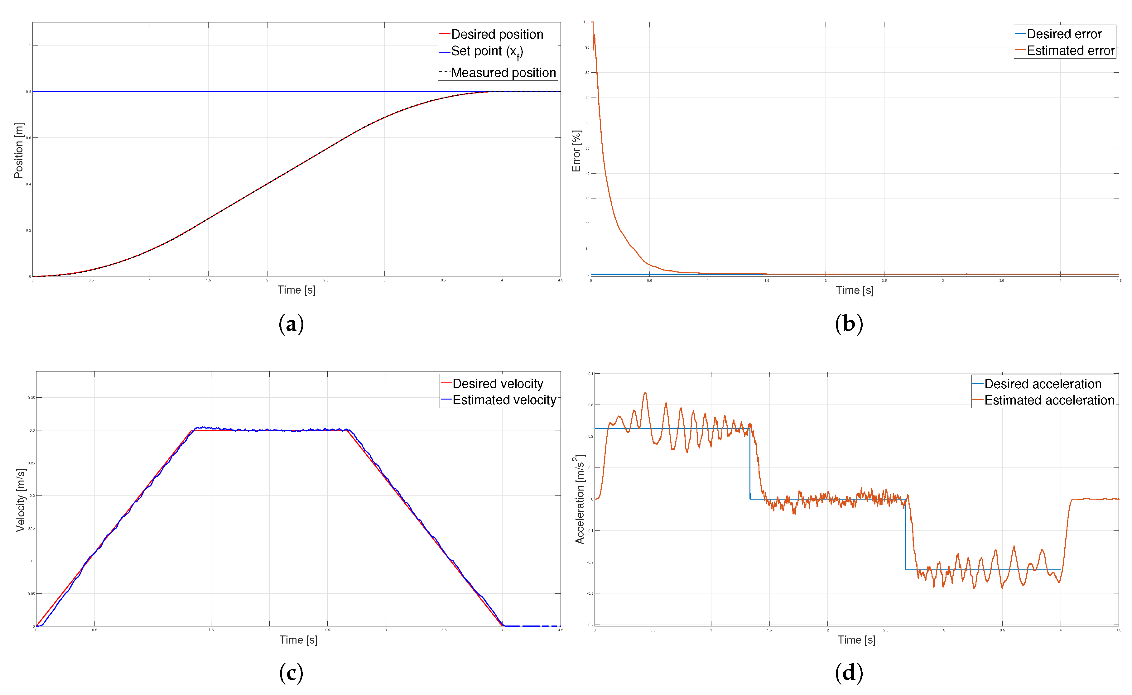
Figure 13.
Trapezoidal velocity profile (a) Control signal, (b) Current (c) Power and (d) Energy.
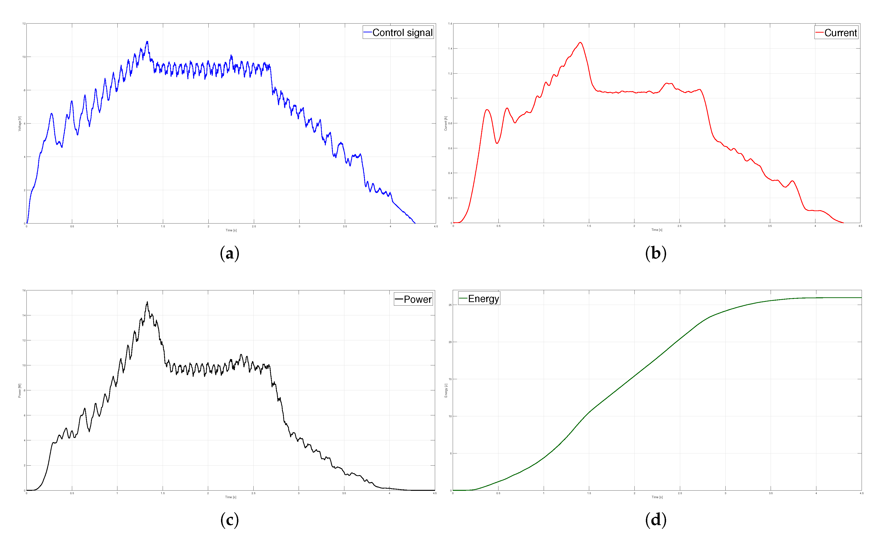
Figure 14.
S-curve velocity profile (a) Position, (b) Error (c) Velocity and (d) Acceleration.
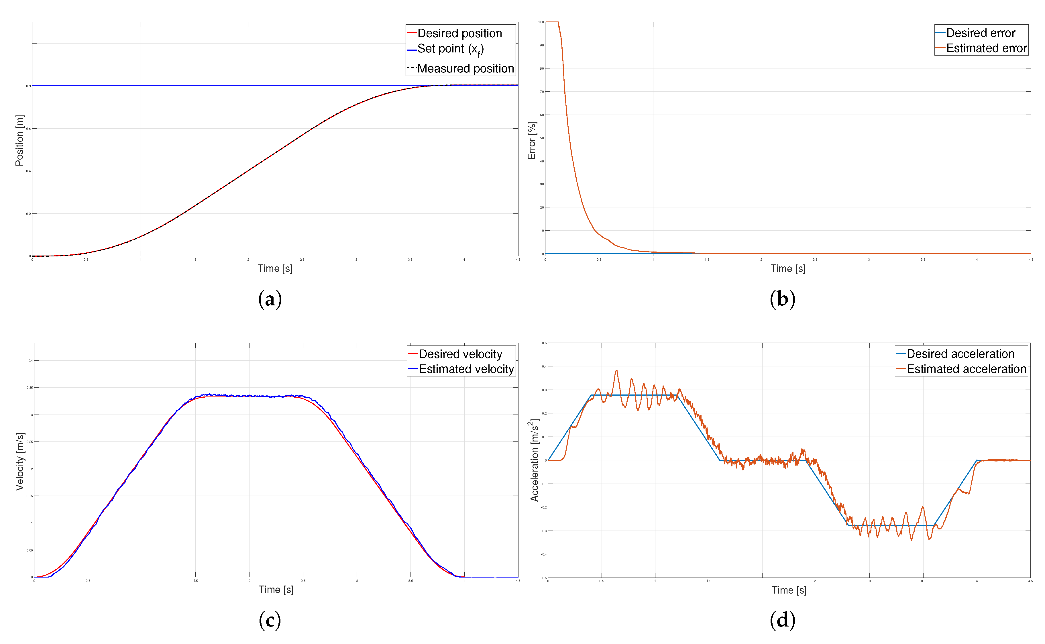
Figure 15.
S-curve velocity profile (a) Control signal, (b) Current (c) Power and (d) Energy.
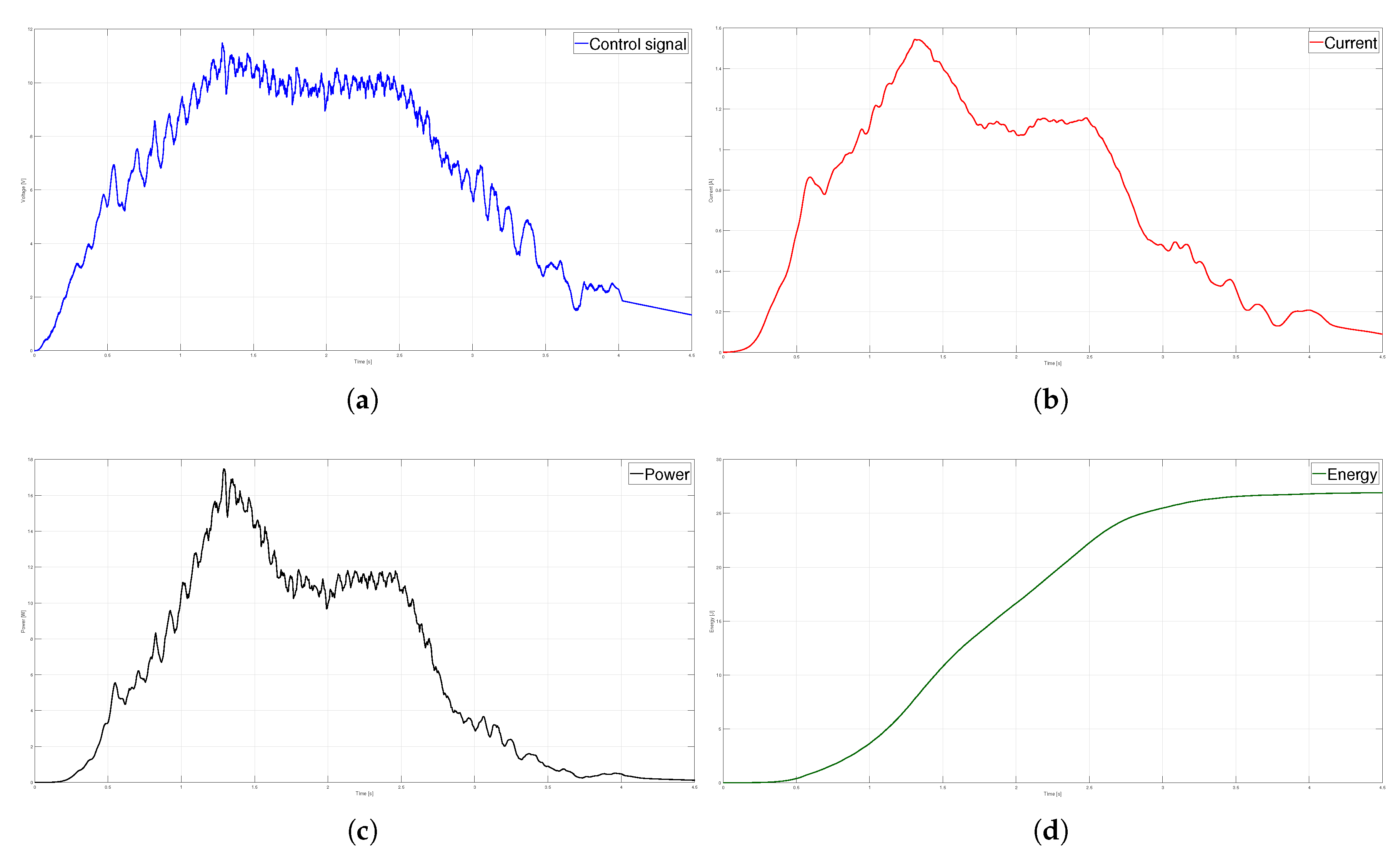
Figure 16.
Error with a load of the three position profiles.
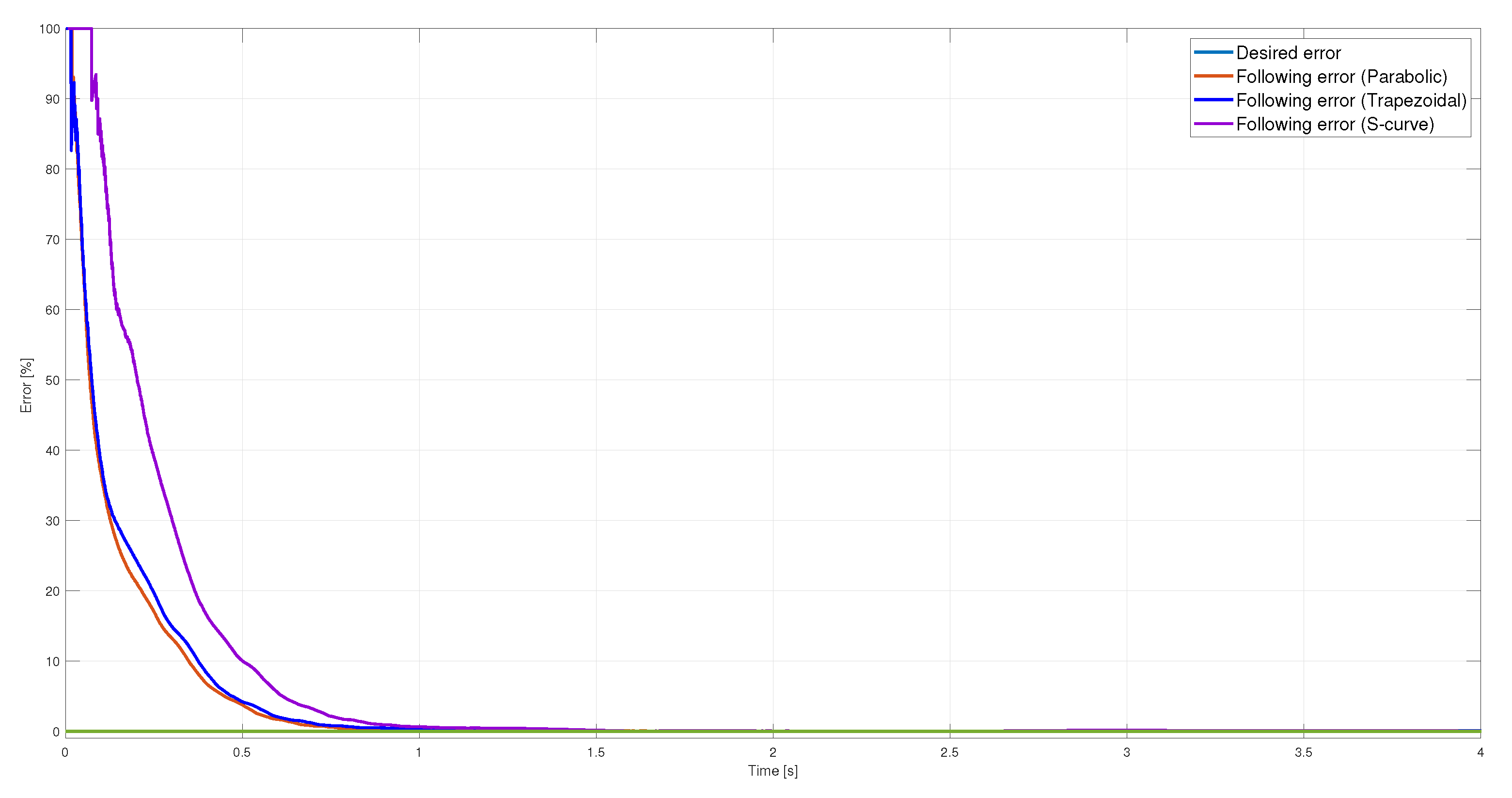
Figure 17.
Control signal with a load of .
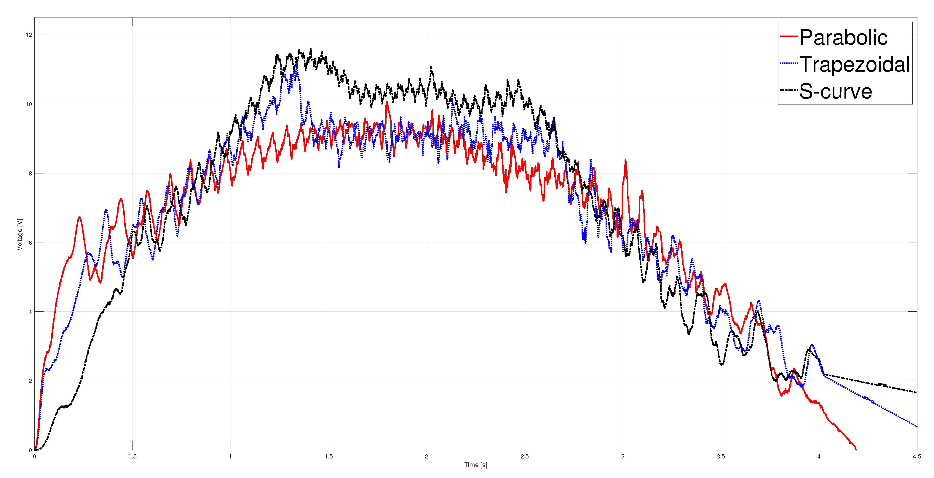
Figure 18.
Current measured with a load of .
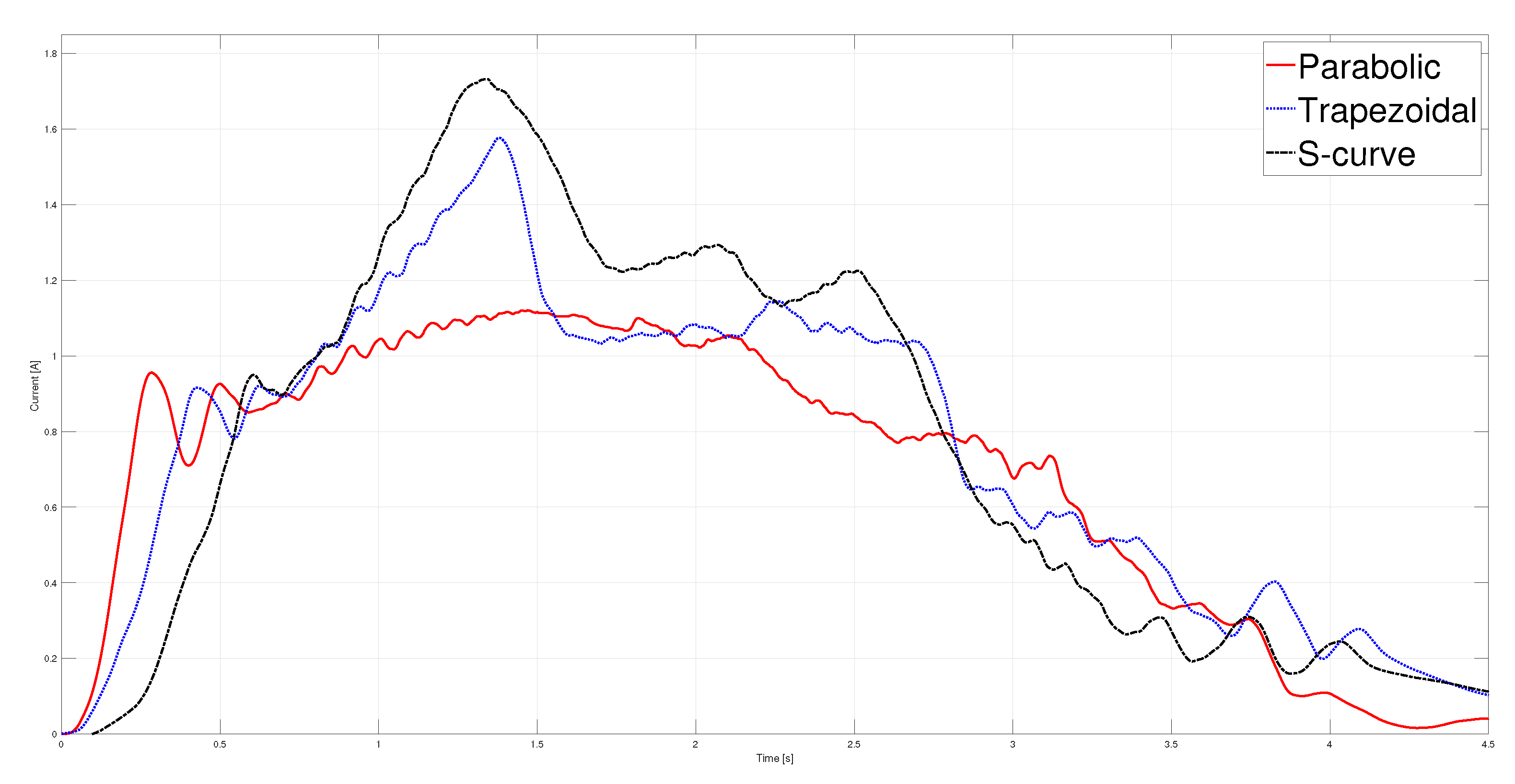
Figure 19.
Power estimated with a load of .
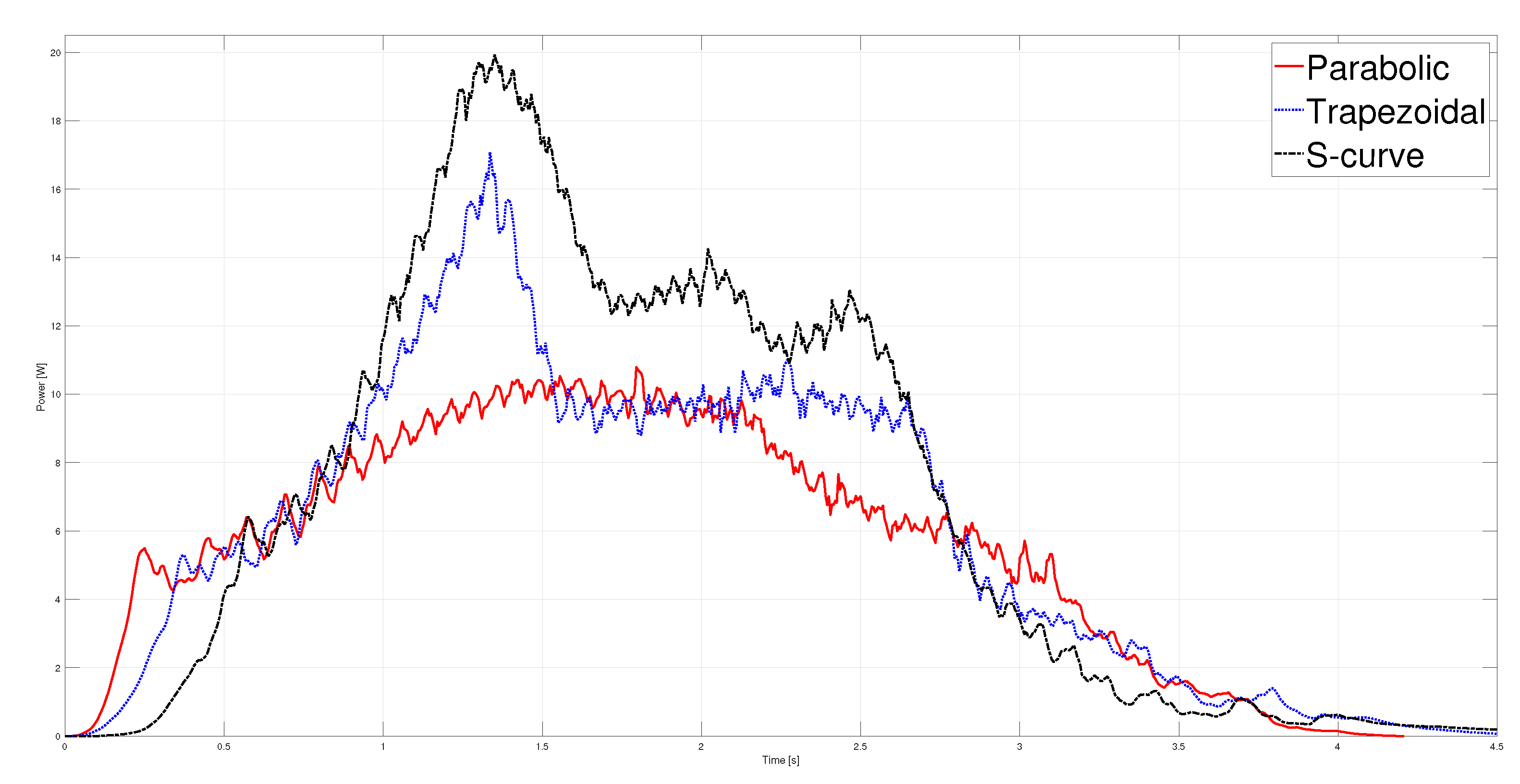
Figure 20.
Energy estimated with a load of .
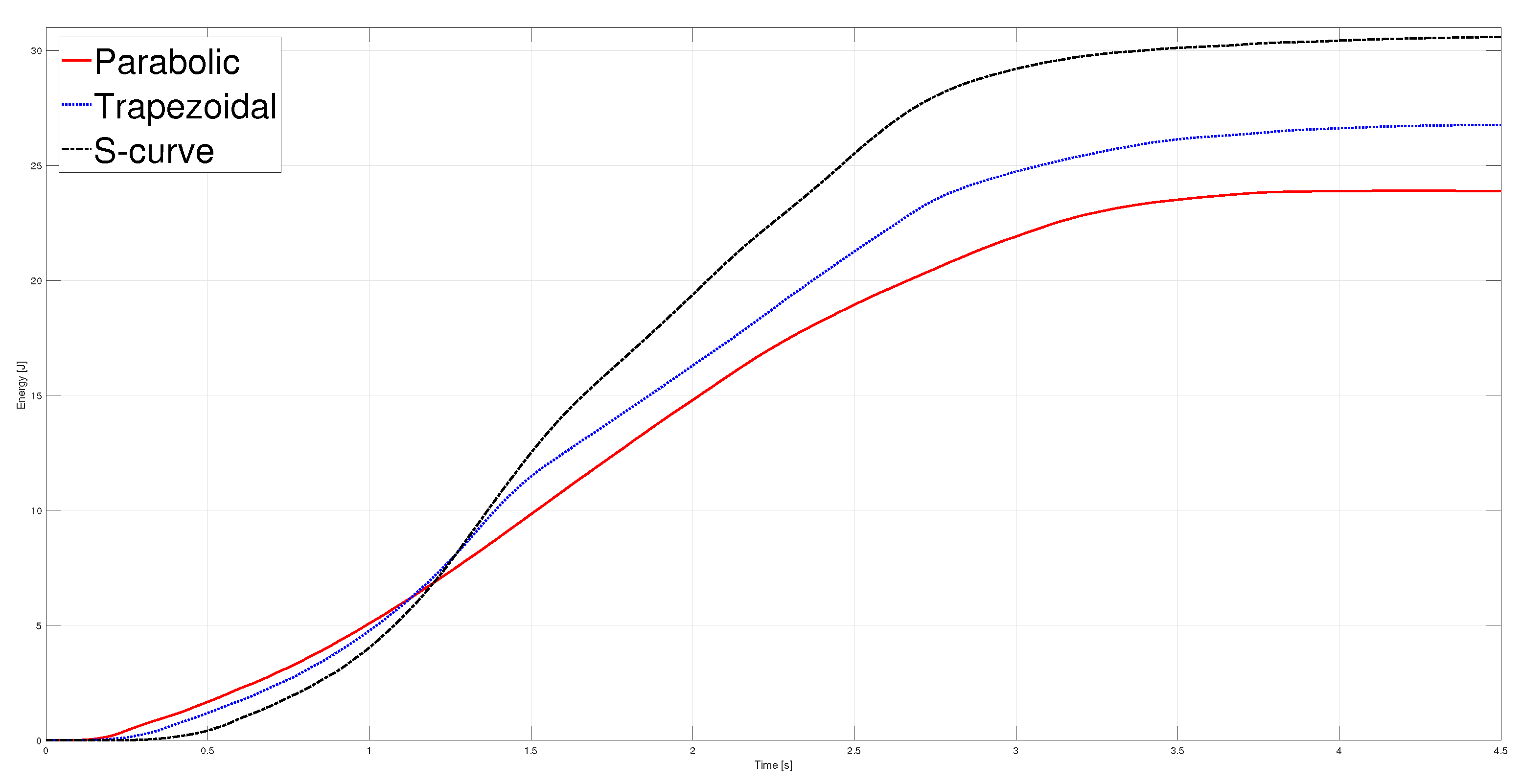
Table 1.
Parameters used to implement the parabolic motion profile.
| Parameter | Value |
|---|---|
| Final position () | m |
| Total time for displacement (T) | 4 s |
| Maximum velocity () | |
| Maximum acceleration () | 0.3 |
Table 2.
Parameters used to implement the trapezoidal motion profile.
| Parameter | Value |
|---|---|
| Final position () | m |
| Total time for displacement (T) | 4 s |
| Acceleration Time () | s |
| Maximum velocity () | |
| Maximum acceleration () |
Table 3.
Parameters used to implement the S-curve velocity profile.
| Parameter | Value |
|---|---|
| Final position () | m |
| Total time for displacement (T) | 4 s |
| Time factor for acceleration () | |
| Time factor for jerk phase () | |
| Acceleration Time () | s |
| Jerk pulse width () | s |
| Maximum velocity () | |
| Maximum acceleration () | |
| Maximum jerk () |
Table 4.
Energy comparison of the three motion profiles.
| Motion profile | Energy (without load) | Energy (with load) |
|---|---|---|
| Parabolic | 23.7044 J | 23.845 J |
| Trapezoidal | 25.9644 J | 26.7616 J |
| S-curve | 26.9525 J | 30.6456 J |
Disclaimer/Publisher’s Note: The statements, opinions and data contained in all publications are solely those of the individual author(s) and contributor(s) and not of MDPI and/or the editor(s). MDPI and/or the editor(s) disclaim responsibility for any injury to people or property resulting from any ideas, methods, instructions or products referred to in the content. |
© 2023 by the authors. Licensee MDPI, Basel, Switzerland. This article is an open access article distributed under the terms and conditions of the Creative Commons Attribution (CC BY) license (http://creativecommons.org/licenses/by/4.0/).
Copyright: This open access article is published under a Creative Commons CC BY 4.0 license, which permit the free download, distribution, and reuse, provided that the author and preprint are cited in any reuse.


