Implementation of ABAQUS User Subroutines for Viscoplasticity of 316 Stainless Steel and Zircaloy-4

Preprint

Article

Implementation of ABAQUS User Subroutines for Viscoplasticity of 316 Stainless Steel and Zircaloy-4

Altmetrics

Downloads

311

Views

Comments

A peer-reviewed article of this preprint also exists.

This version is not peer-reviewed

Submitted:

02 August 2023

Posted:

03 August 2023

You are already at the latest version

Alerts

Abstract

This paper describes the formulations for viscoplasticity of metals based on the Chaboche and Delobelle model. The implementations of the viscoplastic models were detailed herein and then implemented via user subroutines for material models (UMAT) in ABAQUS. Two typical metals, i.e., 316 Stainless Steel and Zircaloy-4, were chosen as examples and their viscoplastic behaviors were captured. Numerical simulations are compared to reported experiments to validate the models and the UMAT codes. Typical viscoplastic behaviors of both metals, such as stress relaxation and creep, were captured well against available experiments. We publicize all the data and codes via: https://github.com/XJTU-Zhou-group/ABAQUS_UMAT_316ss_Zr4.

Keywords:

Subject: Engineering - Mechanical Engineering

1. Introduction

The stress corrosion cracking (SCC) of cladding tube structures caused by pellet clad interaction (PCI) seriously threatens the operation safety of nuclear facilities[1,2]. In order to ensure the structural integrity of nuclear fuel cladding during service, it is necessary to accurately calculate the stress and strain levels of cladding materials in service conditions.

316 Stainless Steel and Zircaloy-4 have become widely used cladding materials due to their excellent high temperature mechanical properties, good oxidation resistance and corrosion resistance[3,4]. Elastic deformation, plastic deformation and high temperature creep are the main deformation behaviors of cladding materials under service conditions. Current fuel rod simulation codes such as FRAPCON, FPIN2, and FALCON typically simplify complex cladding deformation problems into one-dimensional or two-dimensional problems based on axisymmetric, plane strain and one-dimensional radial representation[5,6,7]. However, this method cannot model the multiaxial mechanical behavior of the cladding. Not only that, empirical formulas are generally used in these codes to describe the plasticity and creep behavior of the cladding[8]. This approach greatly limits the generalizability and accuracy of the models despite their simplicity in theory and implementation. Therefore, since 2008, Williamson et al from Idaho National Laboratory (INL) have been developing the multidimensional finite element fuel code BISON[9,10,11]. At the same time, Williamson[12] carried out the multidimensional thermomechanical analysis of multipellet steady and transient light water reactor fuel rod behavior based on ABAQUS commercial finite element code. A power-law creep formulation for describing the deformation behavior of Zircaloy cladding is implemented via ABAQUS user creep subroutine. However, 316 stainless steel and Zircaloy-4 have coupled plasticity and creep behavior at high temperatures[13], so it is necessary to use a unified viscoplastic model to model the mechanical behavior of cladding materials.

The expression of the unified viscoplastic constitutive equation usually includes two aspects: I. the choice of the viscosity function, that is, the expression of the relationship between viscous stress and equivalent plastic strain rate; II. the choice of the hardening equations, that is, the expression of the internal variables[14]. The viscosity equation and the hardening equation are connected through the yield function including overstress to implement the coupled calculation of plasticity and creep. Chaboche and Rousselier[15,16] succeeded in modeling the rate-dependent mechanical behavior of 316 Stainless Steel based on a unified viscoplastic model including nonlinear isotropic hardening rule, nonlinear kinematic hardening rule, and viscosity equation in the form of the power function. Since then, this model has been widely used to model the nonlinear mechanical behavior of metals and polymers, and it is called the Chaboche model[17,18,19,20,21,22]. Unlike 316 Stainless Steel, several experimental studies have been carried out to show that Zircaloy-4 has anisotropic viscoplastic properties due to its microstructural texture[23,24,25,26]. Delobelle[27,28,29] developed a unified viscoplastic constitutive model for Zircaloy-4 modeling by including a viscosity equation in the form of the hyperbolic sine function and three back-stresses playing role successively instead of simultaneously, with some complicated coupling criteria, and he implemented an approach to modeling the anisotropic yield and plastic flow behavior of Zircaloy-4 by using four fourth-order tensors. In this paper, the Chaboche and Delobelle viscoplastic models for 316 stainless steel and Zircaloy-4, respectively, are implemented via the ABAQUS user material subroutine (UMAT). The specific details of the implementation of these two complex constitutive models are given, and numerical simulation results are compared with reported experimental results to validate the model and UMAT code. Two user subroutines developed in this work allowed open-source access to facilitate a more accurate mechanical analysis of cladding structures based on ABAQUS in academia and industry.

2. Viscoplastic Constitutive Equation

2.1. The Framework of Unified Viscoplastic Constitutive Model

Based on the Infinitesimal strain theory, the total strain of the constitutive model can be decomposed into elastic part and viscoplastic part, and the physical mechanism of this method is described in detail in the textbook of Dunne and Petrinic[30]. So the expression for the total strain

ε

is:

ε = ε^{e} + ε^{v p}

(1)

where

ε^{e}

is the elastic strain tensor and

ε^{v p}

is the viscoplastic strain tensor. The constitutive relation of the elastic deformation part can be expressed by the generalized Hooke’s law as follows:

ε^{e} = E^{- 1} : σ

(2)

where

E

is the fourth-order elastic tensor, and

σ

is the Cauchy stress tensor. The plastic strain rate

{\dot{ε}}^{v p}

is expressed based on the associated flow rule as follows:

{\dot{ε}}^{v p} = \dot{p} \frac{\partial f}{\partial σ}

(3)

where f is the yield function, which is equal to the plastic potential function in the associated flow rule and is defined as:

f = f (σ_{e q}, σ_{y}, p, X_{i}, X_{i}), i = 1, 2, \dots

(4)

where

σ_{e q}

is the equivalent stress, which is a certain norm of the Cauchy stress tensor, and the specific expression of the equivalent stress is determined by the yield criterion.

σ_{y}

is the initial yield stress.

X_{i}

and

X_{i}

are internal variables in scalar form and second-order tensor form, respectively, which determine the hardening behavior in the viscoplastic constitutive equation.

\partial f / \partial σ

in Equation (3) means that the direction of the plastic strain rate is perpendicular to the normal direction of the yield surface, which is known as the normality hypothesis of plasticity. p is the equivalent plastic strain, also called accumulated plastic strain, which reflects the loading history of the materials.

\dot{p}

is the equivalent plastic strain rate, indicating the length of the plastic strain increment path in the plastic strain space. The expression of

\dot{p}

under the J2 flow rule is:

\dot{p} = {(\frac{2}{3} {\dot{ε}}^{v p} : {\dot{ε}}^{v p})}^{1 / 2}

(5)

The equivalent plastic strain rate is determined by the viscosity equation

ϕ

\dot{p} = ϕ (σ_{v})

(6)

where

σ_{v}

is the viscous stress, also known as overstress[14], which is the time-dependent part of the total stress in the constitutive equation. The yield function including overstress is as follows:

f = σ_{v} > 0

(7)

Equation (7) shows that the plastic flow behavior described by the unified viscoplastic constitutive model is jointly determined by the hardening rules and the viscosity equation. The viscosity equation can also be defined as:

\{\begin{matrix} \dot{p} = 0 & , f \leq 0 \\ \dot{p} = ϕ (f) > 0 & , f > 0 \end{matrix}

(8)

In summary, to carry out the modeling of material mechanical behavior based on the unified viscoplastic constitutive model, the following three parts need to be determined: I. Yield criterion, that is, the expression of the equivalent stress

σ_{e q}

; II. Hardening rule, that is, the expression of the internal variables

X_{i}

and

X_{i}

; III. The expression of the viscosity equation

φ

2.2. Isotropic Viscoplastic Constitutive Model for 316 Stainless Steel

The viscoplastic constitutive modeling of 316 Stainless Steel is based on the Chaboche model[15,16], and the yield function f expressions based on the von Mises yield criterion, nonlinear isotropic hardening rule and nonlinear kinematic hardening rule are:

\begin{matrix} f & = σ_{e q} - R - σ_{y} \\ = {[\frac{3}{2} (s - α) : (s - α)]}^{1 / 2} - R - σ_{y} \end{matrix}

(9)

where

s

is the deviatoric stress tensor:

s = σ - \frac{1}{3} t r (σ) I

(10)

where

t r (σ)

is the trace of the stress tensor, that is,

t r (σ) = σ_{11} + σ_{22} + σ_{33}

I

is the unit second-order tensor, that is,

I = δ_{i j} {\vec{e}}_{i} {\vec{e}}_{j}

. The scalar internal variable R in Equation (9) is the drag-stress describing the isotropic hardening behavior of the materials, and the second-order tensor internal variable

α

in Equation (9) is the back-stress describing the kinematic hardening behavior of the materials. The expressions of drag-stress R and back-stress

α

evolution are:

\dot{R} = b (Q - R) \dot{p}

(11)

\sum_{i = 1}^{2} α_{i}

(12)

{\dot{α}}_{i} = C_{i} (\frac{2}{3} a_{i} {\dot{ε}}^{v p} - α_{i} \dot{p})

(13)

where b and Q are isotropic hardening parameters, and

C_{1}

C_{2}

a_{1}

and

a_{2}

are kinematic hardening parameters. Equation (13) is the nonlinear kinematic hardening rule proposed by Armstrong and Frederick[31]. Chaboche[15] first used the back-stress expression of the addition of multiple Armstrong-Frederick’s rules to obtain better modeling capabilities of kinematic hardening behavior. The viscosity equation

ϕ

is defined by Norton’s power law:

\dot{p} = ϕ (f) = {(\frac{f}{K})}^{n}

(14)

where K and n are viscoplastic parameters. Substituting Equation (9) and (14) into Equation (3), the expression of viscoplastic strain rate based on the Chaboche model can be obtained as:

{\dot{ε}}^{v p} = \frac{3}{2} {(\frac{f}{K})}^{n} \frac{s - α}{σ_{e q}}, f > 0

(15)

Specific details about the implementation of the isotropic viscoplastic constitutive model for 316 Stainless Steel are detailed in Section 3.2.

2.3. Anisotropic Viscoplastic Constitutive Model for Zircaloy-4

The viscoplastic constitutive modeling of Zircaloy-4 is carried out based on the Delobelle model[27,28,29]. The Hill yield criterion[32] is used to describe the unique anisotropic yield behavior of Zircaloy-4, and the expression of the yield function f is:

f = σ_{e q} = {[\frac{3}{2} (s - α) : M : (s - α)]}^{1 / 2}

(16)

where

M

is the fourth-order anisotropy coefficient tensor. Unlike the 316 Stainless Steel’s model, there is no initial yield stress term in the yield function of the Zircaloy-4 model, indicating that there is no initial elastic domain in Zircaloy-4 model, and the initial Hill yield surface is a point. Considering Voigt notation, we have:

M = (\begin{matrix} M_{11} & M_{12} & M_{13} & 0 & 0 & 0 \\ M_{12} & M_{12} & M_{23} & 0 & 0 & 0 \\ M_{13} & M_{23} & M_{33} & 0 & 0 & 0 \\ 0 & 0 & 0 & M_{44} & 0 & 0 \\ 0 & 0 & 0 & 0 & M_{55} & 0 \\ 0 & 0 & 0 & 0 & 0 & M_{66} \end{matrix}) w i t h \begin{matrix} M_{11} + M_{12} + M_{13} = 0 \\ M_{12} + M_{22} + M_{23} = 0 \\ M_{13} + M_{23} + M_{33} = 0 \end{matrix}

(17)

The modeling is based on the assumption of orthotropy and incompressibility because of the essentially radial orientation of the crystallites in the Zircaloy-4 microstructure[28], which leads to only six independent components of the anisotropy coefficient tensor. The fourth-order coefficient tensors

N

Q

and

R

that describe the anisotropic plastic behavior below also have the same form. The hardening internal variable expression is given by:

\dot{α} = q [\frac{2}{3} Y^{*} N : {\dot{ε}}^{v p} - Q : (α - α^{(1)}) \dot{p}] - [r_{m} {(\frac{α_{e q}}{α_{0}})}^{m_{0}} + r_{m 1} {(\frac{α_{e q}}{α_{0}})}^{m_{1}}] : N : R : \frac{α}{α_{e q}}

(18)

{\dot{α}}^{(1)} = q_{1} [\frac{2}{3} Y^{*} N : {\dot{ε}}^{v p} - Q : (α^{(1)} - α^{(2)}) \dot{p}]

(19)

{\dot{α}}^{(2)} = q_{2} [\frac{2}{3} Y^{*} N : {\dot{ε}}^{v p} - Q : α^{(2)} \dot{p}]

(20)

Y^{*} = Y_{0} + Y_{i s o} + Y_{θ}

(21)

{\dot{Y}}_{i s o} = b_{i s o} (Y_{i s o}^{s a t} - Y_{i s o}) \dot{p}

(22)

{\dot{Y}}_{θ} = b_{θ} (Y_{θ}^{s a t} f (θ) - Y_{θ}) \dot{p}

(23)

f (θ) = 1 - | cos θ |, θ = arccos (\frac{3}{2} \frac{α : R : \dot{α}}{α_{e q} {\dot{α}}_{e q}})

(24)

α_{e q} = {(\frac{3}{2} α : R : α)}^{1 / 2}, {\dot{α}}_{e q} = {(\frac{3}{2} \dot{α} : R : \dot{α})}^{1 / 2}

(25)

where

q_{1}

and

q_{2}

are kinematic hardening parameters, and

b_{i s o}

b_{θ}

Y_{0}

Y_{i s o}^{s a t}

and

Y_{θ}^{s a t}

are scalar internal variable hardening parameters. Equations (18)(19)(20) are kinematic hardening rules in the form of Armstrong-Frederick’s rule. The second term on the right side of Equation (18) is the static recovery term, which is used to describe the hardening recovery behavior independent of plastic strain, and

r_{m}

r_{m 1}

m_{0}

and

m_{1}

are temperature-dependent material parameters. The internal variable

Y^{*}

is the asymptotic value of the back-stress in the evolution process, which has a similar expression to the nonlinear isotropic hardening rule. The viscosity equation

ϕ

is defined as:

\dot{p} = ϕ (f) = ε_{0} {[sinh (\frac{f}{N})]}^{k}

(26)

where

ε_{0}

, N and k are viscoplastic parameters. Creep test results are well described using the viscosity equation in the form of hyperbolic sine function[27]. Substituting Equation (16) and (26) into Equation (3), the expression of viscoplastic strain rate based on the Delobelle model can be obtained as:

{\dot{ε}}^{v p} = \frac{3}{2} ε_{0} {[sinh (\frac{f}{N})]}^{k} \frac{M : (s - α)}{σ_{e q}}, f > 0

(27)

Specific details about the implementation of the anisotropic viscoplastic constitutive model for Zircaloy-4 are detailed in Section 3.3.

3. Computational Algorithm

The unified viscoplastic constitutive model proposed in Section 2 was implemented through the ABAQUS user material subroutine. The stress update algorithms of 316 Stainless Steel model and Zircaloy-4 model are deduced based on semi-implicit integration and return mapping algorithm. The algorithm derived in this section is based on the discretization of the unified viscoplastic constitutive equation, that is, for a time interval

[t_{n}, t_{n + 1}]

, the variable values at

t_{n}

being known and the total strain increment

Δ ε

being given, and the purpose of the algorithm detailed hereafter is to calculate the variable values at time

t_{n + 1}

3.1. Return Mapping Algorithm

The return mapping algorithm is widely used in computational plasticity[30,33]. In general, this approach consists of two parts called “elastic predictor” and “plastic corrector”. The generalized Hooke’s law given by Equation (2) can also be written as:

σ = 2 G ε^{e} + λ t r (ε^{e}) I

(28)

where G is the shear modulus and

λ

is the Lame’s constant. Elastic strain can be decomposed as follows:

ε^{e} = ε_{t}^{e} + Δ ε^{e} = ε_{t}^{e} + Δ ε - Δ ε^{v p}

(29)

For simplicity, the subscript t in this section indicates the variable at time

t_{n}

, and the variable without subscript t indicates the variable at time

t_{n + 1}

. Substitute Equation (29) into Equation (28):

σ = 2 G (ε_{t}^{e} + Δ ε - Δ ε^{v p}) + λ t r (ε_{t}^{e} + Δ ε - Δ ε^{v p}) I

(30)

Considering the incompressible assumption, that is

t r (Δ ε^{v p}) = 0

, Equation (30) can be expressed as:

σ = 2 G (ε_{t}^{e} + Δ ε) + λ t r (ε_{t}^{e} + Δ ε) I - 2 G Δ ε^{v p}

(31)

Let:

σ^{t r i} = 2 G (ε_{t}^{e} + Δ ε) + λ t r (ε_{t}^{e} + Δ ε) I

(32)

where

σ^{t r i}

is the trial stress, also known as “elastic predictor”.

2 G Δ ε^{v p}

is called “plastic corrector”. Substitute Equation (32) into Equation (31):

σ = σ^{t r i} - 2 G Δ ε^{v p}

(33)

After derivation, it can be obtained from the above equation:

σ_{e q} = σ_{e q}^{t r i} - 3 G Δ p

(34)

According to the above derivation, we can get the basic calculation process of the return mapping algorithm as shown in Figure 1:

First, assuming that the total strain increments are all elastic strain increments, the yield function

f^{t r i}

of the trial stress state can be obtained (①-② in Figure 1):

f^{t r i} = σ_{e q}^{t r i} - σ_{y}

(35)

Secondly, if there is

f^{t r i} \leq 0

, it means that the material has not entered the yield state, and the stress

σ_{e q}^{t r i}

corresponding to the trial stress is the updated stress. If there is

f^{t r i} > 0

, it means that the material enters the yield state. At this time, the yield function of the real state should be calculated (②-③ in Figure 1). Considering Equation (34), the yield function of the true state is:

f = σ_{e q} - σ_{y} = (σ_{e q}^{t r i} - 3 G Δ p) - σ_{y} = σ_{v}

(36)

Therefore, obtaining the equivalent plastic strain increment

Δ p

that satisfies both the hardening rules and the viscous equation is the key problem of the stress update algorithm. Specific details about the derivation of the equivalent plastic strain increment

Δ p

of the 316 Stainless Steel model and the Zircaloy-4 model are detailed in Section 3.2 and Section 3.3. Finally, if

Δ p

is obtained, the updated stress can be calculated based on the flow rule and generalized Hooke’s law (①-③ in Figure 1):

Δ ε^{v p} = Δ p n

(37)

Δ σ = E^{- 1} Δ ε^{e} = E^{- 1} : (Δ ε - Δ ε^{v p})

(38)

σ = σ_{t} + Δ σ

(39)

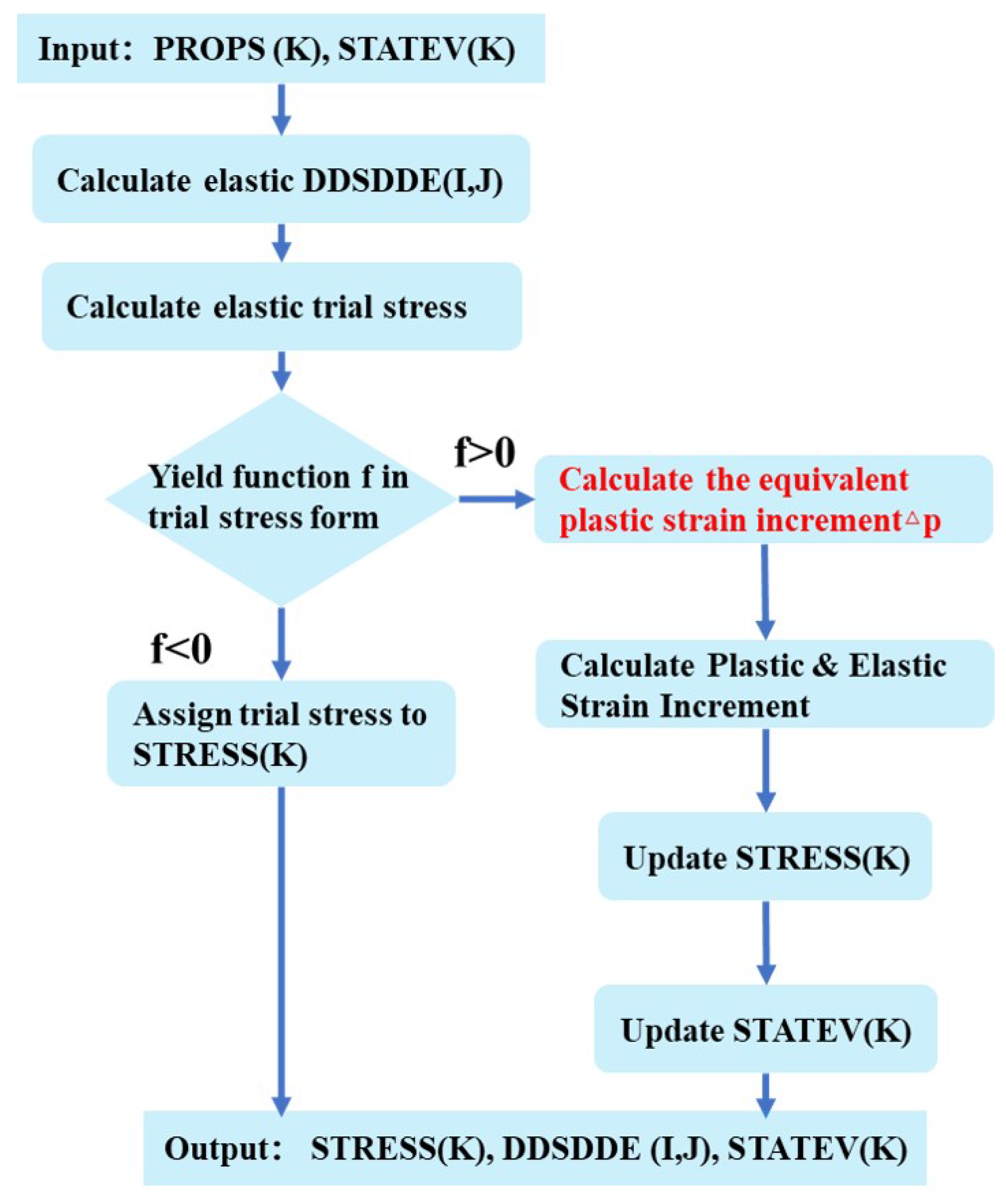
where

n

is the direction of plastic flow, that is,

n = \partial f / \partial σ

. As shown in Equation 38, the algorithm implementation of the constitutive model in this paper is carried out based on the constant stiffness iterative method. The scheme of the return mapping algorithm process is illustrated in Figure 2.

3.2. Stress Update Algorithm of 316 Stainless Steel Model

The isotropic viscoplastic constitutive model for 316 Stainless Steel in Section 2.2 is discretized according to the semi-implicit integration scheme as follows:

f_{(n + 1)} = σ_{e q} - R_{(n + 1)} - σ_{y} = σ_{e q}^{t r i} - 3 G Δ p_{(n + 1)} - R_{(n + 1)} - σ_{y}

(40)

α_{(n + 1)} = α_{(n)} + Δ α_{(n + 1)}

(41)

Δ α_{(n + 1)} = Δ α_{1 (n + 1)} + Δ α_{2 (n + 1)}

(42)

Δ α_{1 (n + 1)} = C_{1} (a_{1} Δ ε_{(n + 1)}^{v p} - α_{1 (n)} Δ p_{(n + 1)})

(43)

Δ α_{2 (n + 1)} = C_{2} (a_{2} Δ ε_{(n + 1)}^{v p} - α_{2 (n)} Δ p_{(n + 1)})

(44)

R_{(n + 1)} = R_{(n)} + Δ R_{(n + 1)}

(45)

Δ R_{(n + 1)} = b (Q - R_{(n)}) Δ p_{(n + 1)}

(46)

According to the Equation 14:

\dot{p} = \frac{d p}{d t} = \frac{Δ p}{Δ t} = ϕ (f) = ϕ (Δ p, α, R)

(47)

Since the expressions of

α

and R both contain

Δ p_{n + 1}

, the Equation 47 is a nonlinear equation about

Δ p_{n + 1}

, which can be solved by Newton-Raphson iterative method. Therefore, it is necessary to derive the Newton-Raphson iteration scheme, rearrange the Equation 47, and let:

ψ (Δ p, α, R) = Δ p - ϕ (Δ p, α, R) Δ t = 0

(48)

Take the first-order Taylor expansion of

ψ

ψ + \frac{\partial ψ}{\partial Δ p} d Δ p + \frac{\partial ψ}{\partial α} : d α + \frac{\partial ψ}{\partial R} d R = 0

(49)

Substituting Equation 48 into Equation 49:

Δ p - ϕ Δ t + (1 - \frac{\partial ϕ}{\partial Δ p} Δ t) d Δ p - \frac{\partial ϕ}{\partial α} : d α Δ t - \frac{\partial ϕ}{\partial R} d R Δ t = 0

(50)

Substituting Equation 11, 12 and 13 into Equation 50, eliminate

d α

d R

and rearrange gives (k is the number of iteration):

d Δ p^{(k + 1)} = \frac{ϕ^{(k)} - Δ p^{(k)} / Δ t}{\frac{1}{Δ t} - {(\frac{\partial ϕ}{\partial Δ p})}^{(k)} + \frac{3}{2} {(\frac{\partial ϕ}{\partial σ_{e q}})}^{(k)} (C_{1} a_{1} + C_{2} a_{2}) - {(\frac{\partial ϕ}{\partial σ_{e q}})}^{(k)} (C_{1} n_{(n)} : α_{1}^{(k)} - C_{2} n_{(n)} : α_{2}^{(k)}) - {(\frac{\partial ϕ}{\partial R})}^{(k)} b (Q - R^{(k)})}

(51)

where:

ϕ^{(k)} = {(\frac{σ_{e q}^{t r i} - 3 G Δ p^{(k)} - R^{(k)} - σ_{y}}{K})}^{n}

(52)

\frac{\partial ϕ}{\partial α} = - \frac{\partial ϕ}{\partial σ_{e q}} n

(53)

{(\frac{\partial ϕ}{\partial σ_{e q}})}^{(k)} = \frac{n}{K} {(\frac{σ_{e q}^{t r i} - 3 G Δ p^{(k)} - R^{(k)} - σ_{y}}{K})}^{n - 1}

(54)

{(\frac{\partial ϕ}{\partial R})}^{(k)} = - \frac{n}{K} {(\frac{σ_{e q}^{t r i} - 3 G Δ p^{(k)} - R^{(k)} - σ_{y}}{K})}^{n - 1}

(55)

{(\frac{\partial ϕ}{\partial Δ p})}^{(k)} = - \frac{3 n G}{K} {(\frac{σ_{e q}^{t r i} - 3 G Δ p^{(k)} - R^{(k)} - σ_{y}}{K})}^{n - 1}

(56)

Calculate the updated internal variables and equivalent plastic strain increment:

Δ p^{(k + 1)} = Δ p^{(k)} + d Δ p^{(k + 1)}

(57)

α^{(k + 1)} = α_{1}^{(k + 1)} + α_{2}^{(k + 1)}

(58)

α_{1}^{(k + 1)} = α_{1 (n)} + Δ α_{1}^{(k + 1)} = α_{1 (n)} + C_{1} (a_{1} n_{(n)} - α_{1 (n)}) Δ p^{(k + 1)}

(59)

α_{2}^{(k + 1)} = α_{2 (n)} + Δ α_{2}^{(k + 1)} = α_{2 (n)} + C_{2} (a_{2} n_{(n)} - α_{2 (n)}) Δ p^{(k + 1)}

(60)

R^{(k + 1)} = R_{(n)} + Δ R^{(k + 1)} = R_{(n)} + b (Q - R_{(n)}) Δ p^{(k + 1)}

(61)

The above is the Newton-Raphson iterative scheme for solving the nonlinear equation about

Δ p_{(n + 1)}

. When

R E S = | Δ p - ϕ (f) Δ t | \to 0

, the iteration ends, that is, the

Δ p

that satisfies both the hardening rules and the viscosity function has been found within the time incremental step

[t_{n}, t_{n + 1}]

Δ p_{(n + 1)} = Δ p^{(k + 1)}

(62)

Calculate the updated plastic strain increment:

Δ ε_{(n + 1)}^{v p} = Δ p_{(n + 1)} n_{(n)}

(63)

where:

n_{(n)} = {(\frac{3}{2} \frac{s - α}{σ_{e q}})}_{(n)}

(64)

Calculate the updated stress:

Δ σ_{(n + 1)} = E^{- 1} : (Δ ε_{(n + 1)} - Δ ε_{(n + 1)}^{v p})

(65)

σ_{(n + 1)} = σ_{(n)} + Δ σ_{(n + 1)}

(66)

3.3. Stress Update Algorithm of Zircaloy-4 Model

The anisotropic viscoplastic constitutive model for Zircaloy-4 in Section 2.3 is discretized according to the semi-implicit integration scheme as follows:

f_{(n + 1)} = σ_{e q} = σ_{e q}^{t r i} - 3 G Δ p_{(n + 1)}

(67)

α_{(n + 1)} = α_{(n)} + Δ α_{(n + 1)}

(68)

α_{(n + 1)}^{(1)} = α_{(n)}^{(1)} + Δ α_{(n + 1)}^{(1)}

(69)

α_{(n + 1)}^{(2)} = α_{(n)}^{(2)} + Δ α_{(n + 1)}^{(2)}

(70)

\begin{matrix} Δ α_{(n + 1)} = & q \{\frac{2}{3} Y_{(n + 1)}^{*} N : Δ ε_{(n + 1)}^{v p} - Q : [α_{(n)} - α_{(n)}^{(1)}] Δ p_{(n + 1)}\} \\ - Δ t [r_{m} {(\frac{α_{e q}}{α_{0}})}^{m_{0}} + r_{m 1} {(\frac{α_{e q}}{α_{0}})}^{m_{1}}] N : R : \frac{α^{(n)}}{α_{e q}} \end{matrix}

(71)

Δ α_{(n + 1)}^{(1)} = q_{1} \{\frac{2}{3} Y_{(n + 1)}^{*} N : Δ ε_{(n + 1)}^{v p} - Q : [α_{(n)}^{(1)} - α_{(n)}^{(2)}] Δ p_{(n + 1)}\}

(72)

Δ α_{(n + 1)}^{(2)} = q_{2} \{\frac{2}{3} Y_{(n + 1)}^{*} N : Δ ε_{(n + 1)}^{v p} - Q : α_{(n)}^{(2)} Δ p_{(n + 1)}\}

(73)

Y_{(n + 1)}^{*} = Y_{0} + Y_{i s o (n + 1)} + Y_{θ (n + 1)}

(74)

Y_{i s o (n + 1)} = Y_{i s o (n)} + Δ Y_{i s o (n + 1)}

(75)

Y_{θ (n + 1)} = Y_{θ (n)} + Δ Y_{θ (n + 1)}

(76)

Δ Y_{i s o (n + 1)} = b_{i s o} (Y_{i s o}^{s a t} - Y_{i s o (n)}) Δ p_{(n + 1)}

(77)

Δ Y_{θ (n + 1)} = b_{θ} (Y_{θ}^{s a t} f {(θ)}_{(n)} - Y_{θ (n)}) Δ p_{(n + 1)}

(78)

According to the Equation 26:

\dot{p} = \frac{Δ p}{Δ t} = ϕ (Δ p, α)

(79)

Similar to the 316 Stainless Steel model, the Newton-Raphson iterative scheme for solving the equivalent plastic strain increment

Δ p_{(n + 1)}

of the Zircaloy-4 model is derived, rearrange the Equation 79, and let:

ψ (Δ p, α) = Δ p - ϕ (Δ p, α) Δ t = 0

(80)

Take the first-order Taylor expansion of

ψ

ψ + \frac{\partial ψ}{\partial Δ p} d Δ p + \frac{\partial ψ}{\partial α} : d α = 0

(81)

Substituting Equation 80 into Equation 81:

Δ p - ϕ Δ t + (1 - \frac{\partial ϕ}{\partial Δ p} Δ t) d Δ p - \frac{\partial ϕ}{\partial α} : d α Δ t = 0

(82)

Substituting Equation 18, 19 and 20 into Equation 82, eliminate

d α

and rearrange gives (k is the number of iteration):

d Δ p^{(k + 1)} = \frac{ϕ^{(k)} - \frac{Δ p^{(k)}}{Δ t} + {(\frac{\partial ϕ}{\partial σ_{e q}})}^{(k)} Δ t [r_{m} {(\frac{α_{e q}}{α_{0}})}^{m_{0}} + r_{m 1} {(\frac{α_{e q}}{α_{0}})}^{m_{1}}] n_{(n)} : N : R : \frac{α^{(k)}}{α_{e q}}}{\frac{1}{Δ t} - {(\frac{\partial ϕ}{\partial Δ p})}^{(k)} + q {(\frac{\partial ϕ}{\partial σ_{e q}})}^{(k)} \{\frac{2}{3} Y^{* (k)} n_{(n)} : N : n_{(n)} - n_{(n)} : Q : [α^{(k)} - α^{(1) (k)}]\}}

(83)

where:

ϕ^{(k)} = {\dot{ε}}_{0} {\{sinh (\frac{σ_{e q}^{t r i} - 3 G Δ p^{(k)}}{N})\}}^{k}

(84)

{(\frac{\partial ϕ}{\partial σ_{e q}})}^{(k)} = \frac{{\dot{ε}}_{0} k}{N} {\{sinh (\frac{σ_{e q}^{t r i} - 3 G Δ p^{(k)}}{N})\}}^{k - 1} cosh (\frac{σ_{e q}^{t r i} - 3 G Δ p^{(k)}}{N})

(85)

{(\frac{\partial ϕ}{\partial Δ p})}^{(k)} = - \frac{3 G {\dot{ε}}_{0} k}{N} {\{sinh (\frac{σ_{e q}^{t r i} - 3 G Δ p^{(k)}}{N})\}}^{k - 1} cosh (\frac{σ_{e q}^{t r i} - 3 G Δ p^{(k)}}{N})

(86)

Calculate the updated internal variables and equivalent plastic strain increment:

Δ p^{(k + 1)} = Δ p^{(k)} + d Δ p^{(k + 1)}

(87)

\begin{matrix} α^{(k + 1)} = & α_{(n)} + Δ α^{(k + 1)} \\ = & α_{(n)} + q \{\frac{2}{3} Y_{(n + 1)}^{*} N : Δ ε_{(n + 1)}^{v p} - Q : [α_{(n)} - α_{(n)}^{(1)}] Δ p_{(n + 1)}\} \\ - Δ t [r_{m} {(\frac{α_{e q}}{α_{0}})}^{m_{0}} + r_{m 1} {(\frac{α_{e q}}{α_{0}})}^{m_{1}}] N : R : \frac{α^{(n)}}{α_{e q}} \end{matrix}

(88)

\begin{matrix} α^{(1) (k + 1)} = & α_{(n)}^{(1)} + Δ α^{(1) (k + 1)} \\ = & α_{(n)}^{(1)} + q_{1} \{\frac{2}{3} Y_{(n + 1)}^{*} N : Δ ε_{(n + 1)}^{v p} - Q : [α_{(n)}^{(1)} - α_{(n)}^{(2)}] Δ p_{(n + 1)}\} \end{matrix}

(89)

\begin{matrix} α^{(2) (k + 1)} = & α_{(n)}^{(2)} + Δ α^{(2) (k + 1)} \\ = & α_{(n)}^{(2)} + q_{2} \{\frac{2}{3} Y_{(n + 1)}^{*} N : Δ ε_{(n + 1)}^{v p} - Q : α_{(n)}^{(2)} Δ p_{(n + 1)}\} \end{matrix}

(90)

Y^{* (k + 1)} = Y_{0} + Y_{i s o}^{(k + 1)} + Y_{θ}^{(k + 1)}

(91)

Y_{i s o}^{(k + 1)} = Y_{i s o (n)} + Δ Y_{i s o}^{(k + 1)} = Y_{i s o (n)} + b_{i s o} (Y_{i s o}^{s a t} - Y_{i s o (n)}) Δ p^{(k + 1)}

(92)

Y_{θ}^{(k + 1)} = Y_{θ (n)} + Δ Y_{θ}^{(k + 1)} = Y_{θ (n)} + b_{θ} (Y_{θ}^{s a t} f {(θ)}_{(n)} - Y_{θ (n)}) Δ p^{k + 1}

(93)

The iteration ends when

R E S = | Δ p - ϕ (f) Δ t | \to 0

Δ p_{(n + 1)} = Δ p^{(k + 1)}

(94)

The plastic strain increment is then determined from:

Δ ε_{(n + 1)}^{v p} = Δ p_{(n + 1)} n_{(n)}

(95)

where:

N_{(n)} = {(\frac{3}{2} \frac{M : (s - α)}{σ_{e q}})}_{(n)}

(96)

Calculate the updated stress as Equation 65 and 66.

4. Verification and Validation of FE Modeling and UMAT Code

In order to verify the accuracy of the unified viscoplastic constitutive model and its algorithm implementation, numerical simulations of the viscoplastic mechanical behavior of materials were carried out using the ABAQUS user material subroutine of the 316 Stainless Steel model and the Zircaloy-4 model, and compared with the experimental results. The reported experimental studies are described in the cylindrical coordinate system due to the use of hollow circular cross-section rod specimens[16,18,28]. In order to correspond to the Cartesian coordinates system adopted for the theory and modeling in this paper, so we have:

11 = x = r

22 = y = θ

33 = z = z

12 = x y = r θ

13 = x z = r z

and

23 = y z = θ z

4.1. 316 Stainless Steel

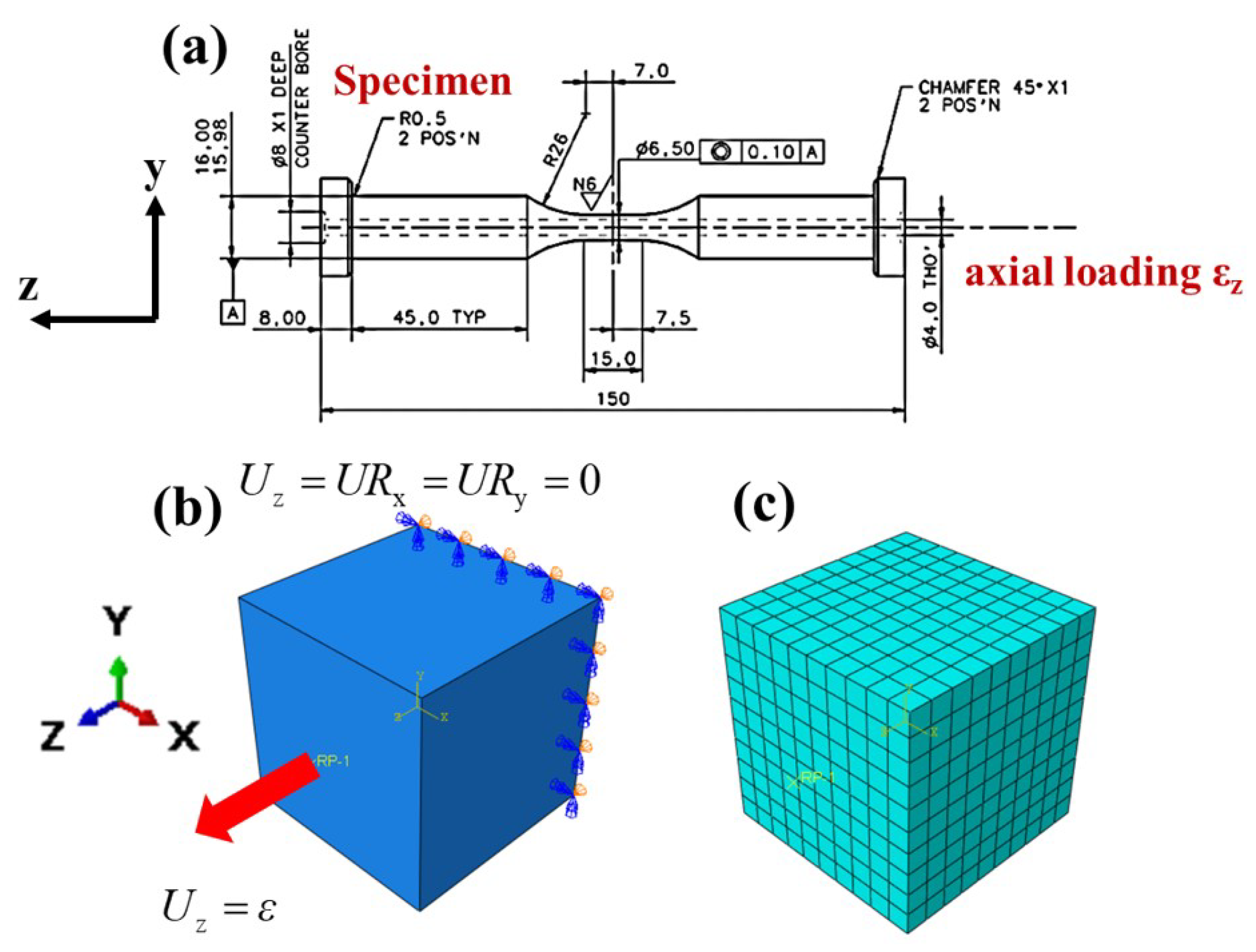
Chaboche et al[16] used the 316 Stainless Steel hollow circular cross-section rod specimen shown in Figure 3a to carry out uniaxial tensile tests at room temperature for different strain rates, and stress relaxation test at room temperature were also carried out:

The gauge length of the specimen is a unidirectional stress state along the axis z-direction, so the finite element model is considered as a simple

1 \times 1 \times 1

cube, as shown in Figure 3b. The displacement boundary condition is defined in the z-direction of the model to simulate the uniaxial tensile behavior of the materials, and the symmetric boundary condition in the z-direction is applied on the other side. The model has meshed into 1000 C3D8 elements for simulation, as shown in Figure 3c. The material constants of 316 Stainless Steel at room temperature are shown in Table 1:

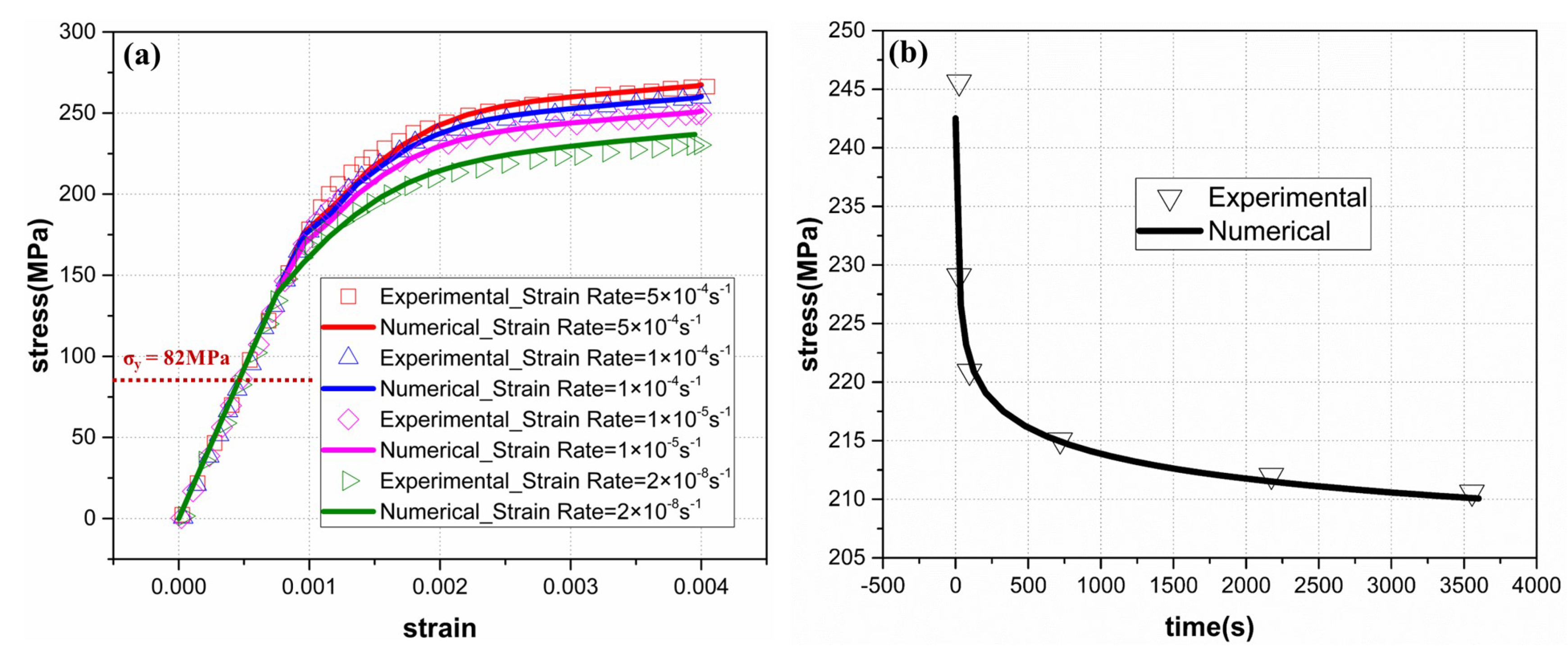
Figure 4a is the stress-strain curve of 316 Stainless Steel for different strain rates at room temperature:

The numerical simulation results are in good agreement with the experimental results, and the 316 Stainless Steel modeling and UMAT code are verified. When the stress is less than the yield stress

σ_{y}

, the stress-strain curves for different strain rates overlap, and the stress-strain behavior of the materials show rate-dependence only after yielding, which is the basic characteristic of the elasto-viscoplastic constitutive model. From Equation 7 and 14, we have:

σ_{v} = K {\dot{p}}^{1 / n}

(97)

that is:

σ \propto \dot{ε}

(98)

The above equation shows that the stress of the materials is positively correlated with the strain rate, that is, the greater the strain rate when the material is loaded, the greater the stress when the material is loaded to the same strain, which is consistent with the phenomenon described by the stress-strain curve in Figure 4a. Figure 4b shows the stress relaxation curve of 316 Stainless Steel at room temperature, and the numerical simulation results are in good agreement with the experiment. When the materials maintain a certain strain, as time increases, the stress gradually decreases until the stress caused by the viscosity of the material disappears completely. It is worth noting that the viscous stress is caused by the plastic strain as shown in Equation 97. Therefore, if the materials be held at a strain level corresponding to stress that does not reach the yield stress, materials will not exhibit stress relaxation behavior.

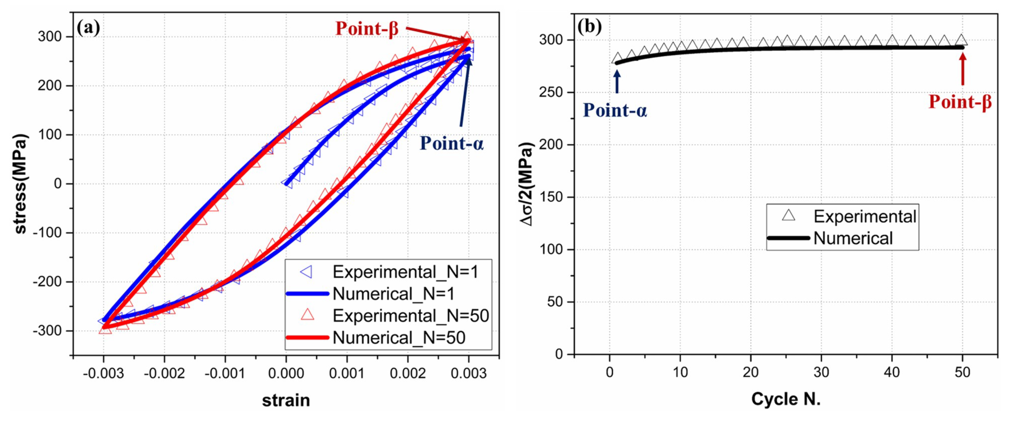
Hyde et al[18] used the 316 Stainless Steel hollow circular cross-section rod specimen shown in Figure 3a to carry out the low cycle fatigue test (LCF test) at 550 °C. The test is controlled by strain, the loading waveform is triangular wave, the strain amplitude is

0.006

, the strain ratio is

- 1

, and the period is

80 s

. Numerical simulations also use the finite element model shown in Figure 3b and c, setting the same displacement boundary conditions in the z-direction as the LCF test. As shown in Figure 5a, the stress-strain loops predicted by the model for the first and fiftieth cycles are in good agreement with the test:

Figure 5b shows the relationship between the half stress range and the number of cycles, and the numerical simulation results are in good agreement with the experimental results. The model successfully predicted the cyclic hardening behavior of 316 Stainless Steel at high temperature. The combined isotropic and kinematic hardening rules governing the cyclic hardening behavior in the constitutive equations are shown in Equation 11, 12 and 13.

4.2. Zircaloy-4

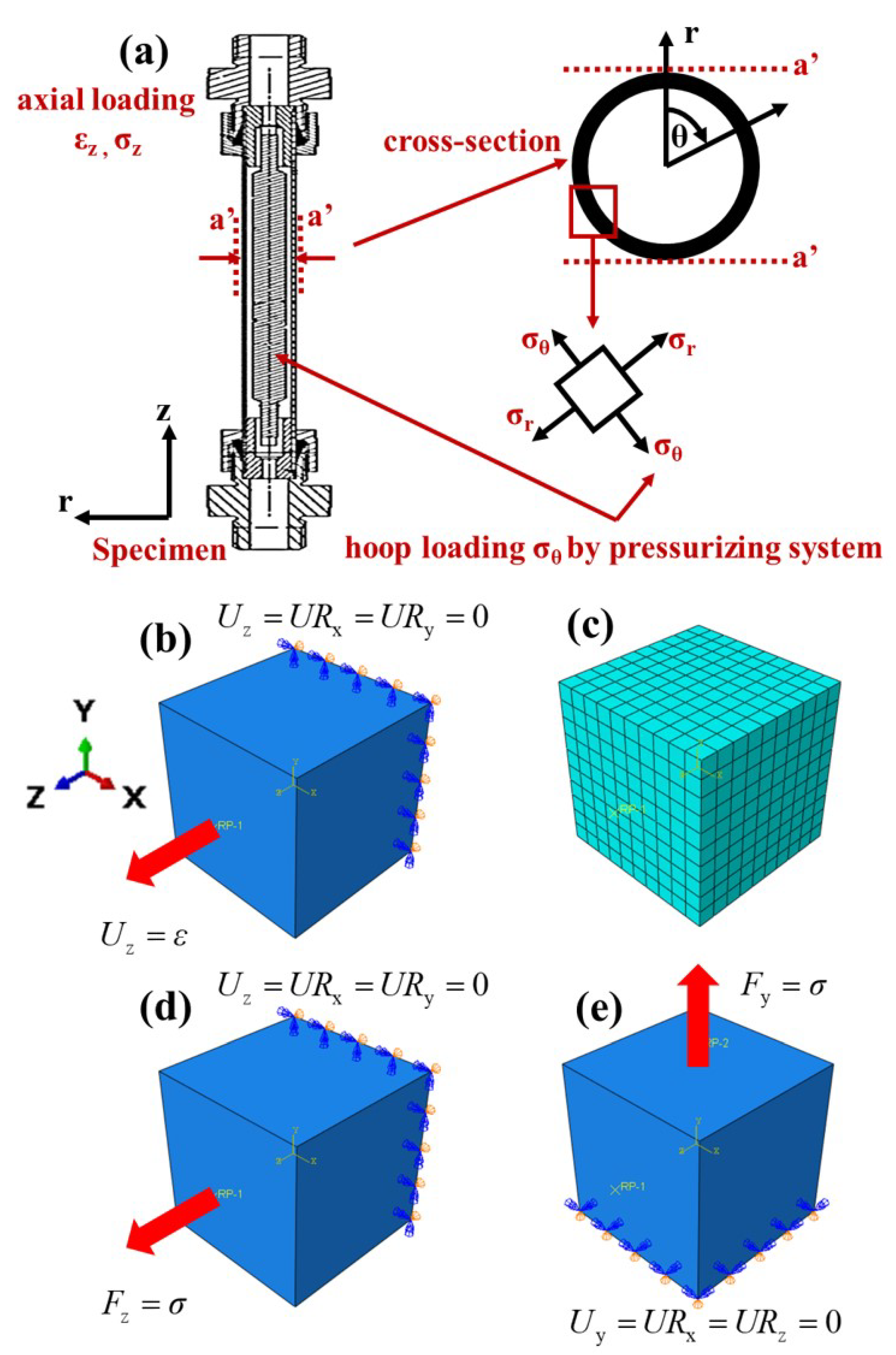
Delobelle et al[28] used the Zircaloy-4 circular tube specimen shown in Figure 6a to carry out the uniaxial tensile test for different strain rates and creep test in the axial and hoop directions, the tests were carried out at

350 ° C

In the uniaxial tensile test, the circular tube specimen is subjected to a displacement-controlled loading in the z-direction, and the gauge length of the specimen is a unidirectional stress state along the z-direction, so the finite element model is considered as a simple

1 \times 1 \times 1

cube, as shown in Figure 6b. The displacement boundary condition is defined in the z-direction of the model to simulate the uniaxial tensile behavior of the specimen, and the symmetric boundary condition in the z-direction is applied on the other side. The model has meshed into 1000 C3D8 elements for simulation, as shown in Figure 6c. Two different metallurgical states of Zircaloy-4 were used for the test, namely recrystallized (R state) Zircaloy-4 and cold worked stress relieved (CWSR state) Zircaloy-4. The Zircaloy-4 material constants of the two metallurgical states are shown in Table 2:

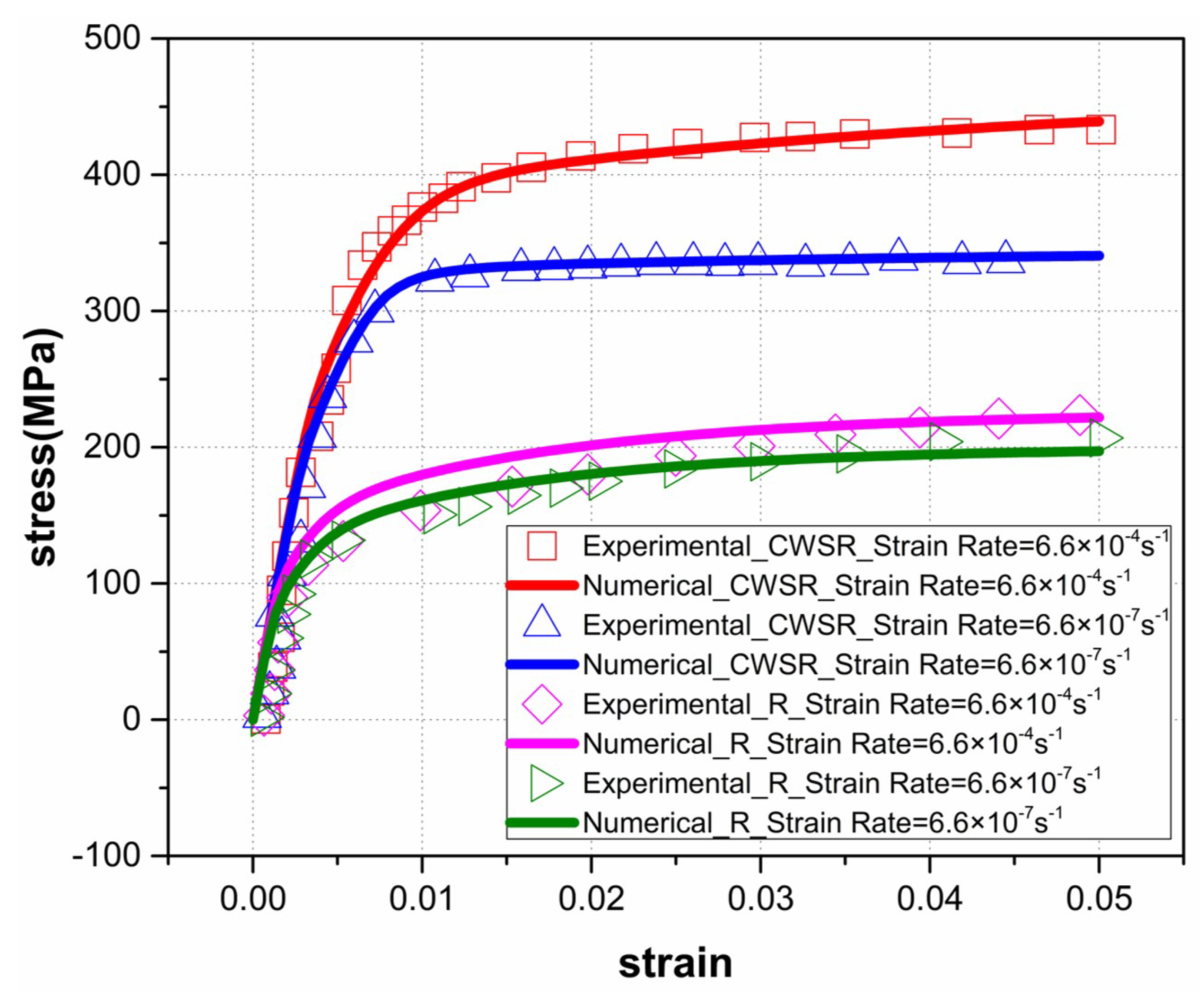
Compared with Zircaloy-4 in the CWSR state, the material constants of Zircaloy-4 in the R state lack the parameters of the internal variable

Y_{i s o}

shown in the Equation 22, because the Zircaloy-4 in the R state has cyclic loading stability, and

Y_{i s o}

mainly controls the cyclic hardening behavior of the materials. Therefore, the

Y_{i s o}

term is not considered in the modeling of the viscoplastic mechanical behavior of Zircaloy-4 in R state, and the relevant parameters can be set to zero when using UMAT to carry out the simulation of Zircaloy-4 in R state. Figure 7 shows the stress-strain curves of R state and CWSR state Zircaloy-4 for different strain rates at 350°C:

The numerical simulation results are in good agreement with the experimental results, which verifies the correctness of Zircaloy-4 modeling and UMAT code. According to Equation 7 and 26, we have:

σ_{v} = N {sinh}^{- 1} [{(\frac{\dot{p}}{{\dot{ε}}_{0}})}^{1 / k}]

(99)

Similar to 316 Stainless Steel, the stress of Zircaloy-4 is positively correlated with the strain rate (Equation 98), that is, the greater the strain rate when the material is loaded, the greater the stress when the material is loaded to the same strain, which is consistent with the phenomenon described by the stress-strain curve in Figure 7.

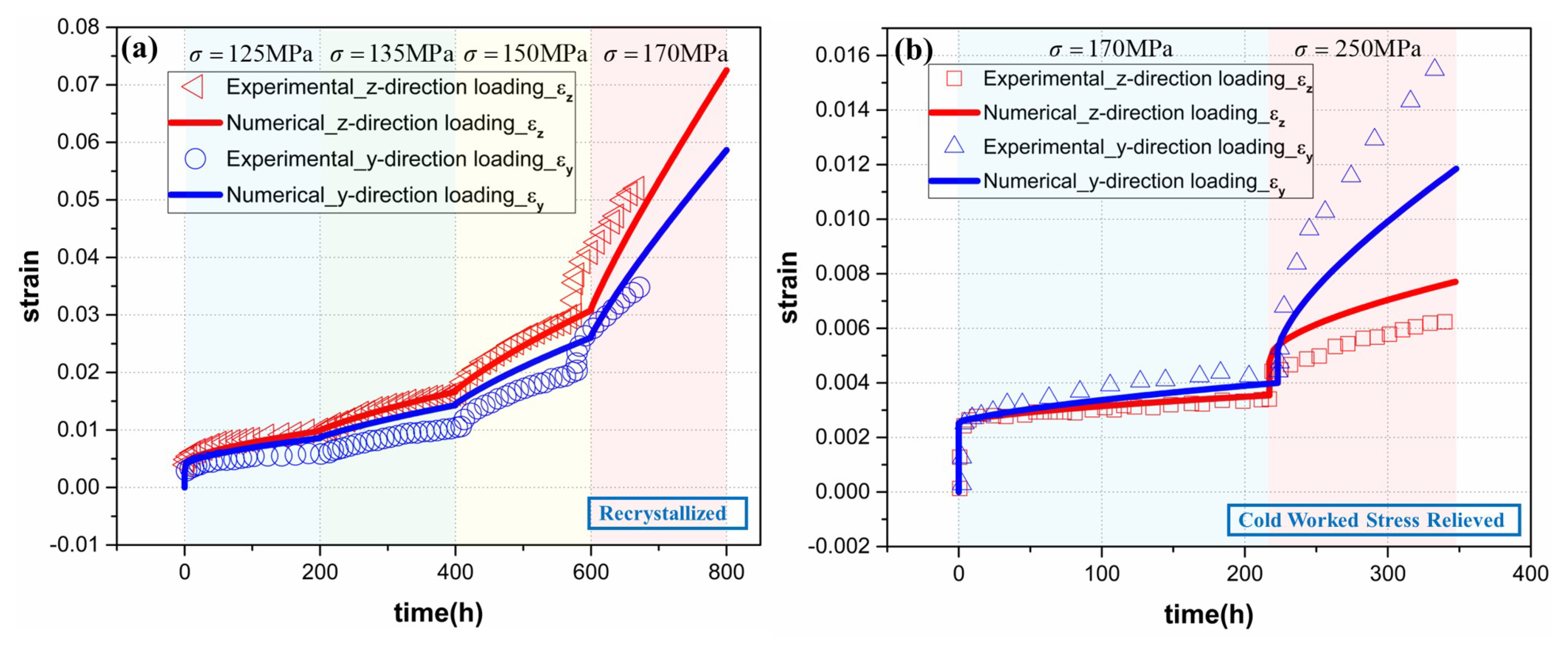
Based on the test device in Figure 6a, Delobelle et al[28] carried out uniaxial creep tests of Zircaloy-4 in different material orientations. The loading method of the uniaxial creep test in the z-direction is the same as that of the uniaxial tensile test in the z-direction, and the force sensor located at the clamping end of the specimen ensures that the Zircaloy-4 round tube is in a constant stress loading state. The hoop creep loading of the Zircaloy-4 circular tube is controlled by the pressurizing system, and a constant hoop stress is applied to the specimen to carry out the creep test. This loading scheme is closer to the service conditions of materials used in nuclear fuel cladding structures. Since the gauge length of the Zircaloy-4 tube is a unidirectional stress state when the creep tests are carried out in two directions, the finite element model is still considered as a simple

1 \times 1 \times 1

cube. As shown in Figure 6d, the stress boundary condition is defined in the z-direction of the model to simulate the uniaxial creep behavior of the specimen in the axial direction, and the symmetrical boundary condition in the z-direction is applied on the other side. As shown in Figure 6e, the stress boundary condition is defined in the y-direction of the model to simulate the uniaxial creep behavior of the specimen in the hoop direction, and the symmetric boundary condition in the y-direction is applied on the other side. The model has meshed into 1000 C3D8 elements for simulation, as shown in Figure 6c. The creep stresses of Zircaloy-4 in the R state are

125 M P a

135 M P a

150 M P a

, and

170 M P a

, respectively, and the creep stresses of Zircaloy-4 in the CWSR state are

170 M P a

and

250 M P a

, and each creep stress level is maintained for 200 hours and then increased to the next stress level. Figure 8 shows the incremental uniaxial creep curves of Zircaloy-4 in R state and CWSR state at

350 ° C

The numerical simulation results are basically consistent with the experimental results. Neglecting the uncertainties in the loading control and deformation acquisition of the high-temperature creep test, the strain amplitudes, as well as the flow directions, are on the whole correctly modeled, so the simulation results are generally acceptable.

5. Conclusions

Within this study, we present the implementation of the ABAQUS user material subroutines of the Chaboche unified viscoplastic constitutive model and the Delobelle unified viscoplastic constitutive model for 316 Stainless Steel and Zircaloy-4. The Chaboche model includes nonlinear isotropic hardening, nonlinear kinematic hardening, and a viscosity equation in the form of a power function. Delobelle model includes a viscosity equation in the form of the hyperbolic sine function and three back-stresses playing roles successively instead of simultaneously, and the anisotropic viscoplastic behavior of the materials is considered. The derivation of the stress update algorithm that implements the Chaboche model and the Delobelle model is based on the return mapping algorithm and the semi-implicit integration scheme, and the UMAT user subroutines for 316 Stainless Steel and Zircaloy-4 are developed. The simulation results with the use of subroutines were verified against existing experimental data from the literature. The models and UMAT subroutines successfully simulated the viscoplastic mechanical behavior of 316 Stainless Steel and Zircaloy-4.

The simulation results successfully captured the rate-dependent stress-strain behavior, stress relaxation behavior and cyclic hardening behavior of 316 Stainless Steel, and the rate-dependent stress-strain behavior and anisotropic creep behavior of Zircaloy-4 in two metallurgical states. This demonstrates that the simulation capability of the user subroutines we developed covers various loading conditions of the cladding materials in service. We hope our efforts provide useful material models and available source codes for users from academia or industry to carry out more accurate mechanical analysis of cladding structures.

Author Contributions

Methodology, X.Y., J.Z.; software, X.Y.; formal analysis, X.Y.; investigation, X.Y.; resources, J.Z.; writing—original draft preparation, X.Y.; writing—review and editing, J.Z.; visualization, X.Y.; supervision, J.Z.; project administration, J.Z. All authors have read and agreed to the published version of the manuscript.

Data Availability Statement

The raw/processed data required to reproduce these findings are available to download from https://github.com/XJTU-Zhou-group/ABAQUS_UMAT_316ss_Zr4.

Acknowledgments

This research is supported by National Natural Science Foundation of China (grant 11972277) and by Science and Technology on Reactor System Design Technology Laboratory (LRSDT2021205).

Conflicts of Interest

The authors declare no conflict of interest.

References

Cox, B. Pellet-clad interaction (PCI) failures of zirconium alloy fuel cladding—a review. Journal of nuclear materials 1990, 172, 249–292. [Google Scholar] [CrossRef]
Jezequel, T.; Auzoux, Q.; Le Boulch, D.; Bono, M.; Andrieu, E.; Blanc, C.; Chabretou, V.; Mozzani, N.; Rautenberg, M. Stress corrosion crack initiation of Zircaloy-4 cladding tubes in an iodine vapor environment during creep, relaxation, and constant strain rate tests. Journal of Nuclear Materials 2018, 499, 641–651. [Google Scholar] [CrossRef]
Hallstadius, L.; Johnson, S.; Lahoda, E. Cladding for high performance fuel. Progress in Nuclear Energy 2012, 57, 71–76. [Google Scholar] [CrossRef]
Azevedo, C.d.F. Selection of fuel cladding material for nuclear fission reactors. Engineering Failure Analysis 2011, 18, 1943–1962. [Google Scholar] [CrossRef]
Berna, G.; Beyer, G.; Davis, K.; Lanning, D. FRAPCON-3: A computer code for the calculation of steady-state, thermal-mechanical behavior of oxide fuel rods for high burnup. Technical report, US Nuclear Regulatory Commission (NRC), Washington, DC (United States). Div. of Systems Technology; Pacific Northwest National Lab.(PNNL), Richland, WA (United States); Idaho National Lab.(INL), Idaho Falls, ID (United States), 1997.
Hughes, T. FPIN2 analysis of metal fueled pins. Technical report, Argonne National Lab.(ANL), Argonne, IL (United States), 1985.
Yagnik, S.; Rashid, Y.; Dunham, R.; Montgomery, R. Fuel Analysis and Licensing Code: FALCON MOD01, Volume 1: Theoretical and Numerical Bases. EPRI, Palo Alto, CA, USA 2004, 1011307. [Google Scholar]
Allison, C.; Berna, G.; Chambers, R.; Coryell, E.; Davis, K.; Hagrman, K.; McComas, M. SCDAP/RELAP5/MOD3. 1 Code Manual Volume IV: MATPRO. NUREG/CR 1993, 6150, 20555–0001. [Google Scholar]
Williamson, R.L.; Hales, J.; Novascone, S.; Tonks, M.; Gaston, D.; Permann, C.; Andrs, D.; Martineau, R. Multidimensional multiphysics simulation of nuclear fuel behavior. Journal of Nuclear Materials 2012, 423, 149–163. [Google Scholar] [CrossRef]
Newman, C.; Hansen, G.; Gaston, D. Three dimensional coupled simulation of thermomechanics, heat, and oxygen diffusion in UO2 nuclear fuel rods. Journal of Nuclear Materials 2009, 392, 6–15. [Google Scholar] [CrossRef]
Williamson, R.L.; Hales, J.D.; Novascone, S.R.; Pastore, G.; Gamble, K.A.; Spencer, B.W.; Jiang, W.; Pitts, S.A.; Casagranda, A.; Schwen, D.; et al. BISON: A flexible code for advanced simulation of the performance of multiple nuclear fuel forms. Nuclear Technology 2021, 207, 954–980. [Google Scholar] [CrossRef]
Williamson, R. Enhancing the ABAQUS thermomechanics code to simulate multipellet steady and transient LWR fuel rod behavior. Journal of Nuclear Materials 2011, 415, 74–83. [Google Scholar] [CrossRef]
Phan, V.T.; Messner, M.; Sham, T.L. A unified engineering inelastic model for 316H stainless steel. In Proceedings of the Pressure Vessels and Piping Conference; 2019. [Google Scholar] [CrossRef]
Chaboche, J.L. A review of some plasticity and viscoplasticity constitutive theories. International journal of plasticity 2008, 24, 1642–1693. [Google Scholar] [CrossRef]
Chaboche, J.; Rousselier, G. On the plastic and viscoplastic constitutive equations—Part I: Rules developed with internal variable concept. Journal of Pressure Vessel Technology 1983. [Google Scholar] [CrossRef]
Chaboche, J.L.; Rousselier, G. On the plastic and viscoplastic constitutive equations—Part II: application of internal variable concepts to the 316 stainless steel. Journal of Pressure Vessel Technology 1983. [Google Scholar] [CrossRef]
Chaboche, J.L. Constitutive equations for cyclic plasticity and cyclic viscoplasticity. International journal of plasticity 1989, 5, 247–302. [Google Scholar] [CrossRef]
Hyde, C.J.; Sun, W.; Leen, S.B. Cyclic thermo-mechanical material modelling and testing of 316 stainless steel. International Journal of Pressure Vessels and Piping 2010, 87, 365–372. [Google Scholar] [CrossRef]
Lim, L.; Dunne, F. The effect of volume fraction of reinforcement on the elastic-viscoplastic response of metal-matrix composites. International journal of mechanical sciences 1995, 38, 19–39. [Google Scholar] [CrossRef]
Hyde, C.J.; Sun, W.; Hyde, T.; Rouse, J.; Farragher, T.; O’Dowd, N.P.; Leen, S. Cyclic viscoplasticity testing and modeling of a service-aged P91 steel. Journal of Pressure Vessel Technology 2014, 136, 044501. [Google Scholar] [CrossRef]
Miled, B.; Doghri, I.; Delannay, L. Coupled viscoelastic–viscoplastic modeling of homogeneous and isotropic polymers: Numerical algorithm and analytical solutions. Computer methods in applied mechanics and engineering 2011, 200, 3381–3394. [Google Scholar] [CrossRef]
Tian, J.; Li, J.; Xie, H.; Yang, Y.; Kan, Q. Finite element implementation of a temperature-dependent cyclic plastic model for SA508-3 steel. Metals 2018, 8, 955. [Google Scholar] [CrossRef]
Murty, K.L.; Charit, I. Texture development and anisotropic deformation of zircaloys. Progress in nuclear energy 2006, 48, 325–359. [Google Scholar] [CrossRef]
Murty, K.L.; Adams, B.L. Biaxial creep of textured zircaloy I: experimental and phenomenological descriptions. Materials Science and Engineering 1985, 70, 169–180. [Google Scholar] [CrossRef]
Grosjean, C.; Poquillon, D.; Salabura, J.C.; Cloué, J.M. Experimental creep behaviour determination of cladding tube materials under multi-axial loadings. Materials Science and Engineering: A 2009, 510, 332–336. [Google Scholar] [CrossRef]
Rautenberg, M.; Poquillon, D.; Pilvin, P.; Grosjean, C.; Cloué, J.M.; Feaugas, X. Thermal isocreep curves obtained during multi-axial creep tests on recrystallized Zircaloy-4 and M5™ alloy. Nuclear Engineering and Design 2014, 269, 33–37. [Google Scholar] [CrossRef]
Delobelle, P. Synthesis of the elastoviscoplastic behavior and modelization of an austenitic stainless steel over a large temperature range, under uniaxial and biaxial loadings, part II: Phenomenological modelization. International journal of plasticity 1993, 9, 87–118. [Google Scholar] [CrossRef]
Delobelle, P.; Robinet, P.; Geyer, P.; Bouffioux, P. A model to describe the anisotropic viscoplastic behaviour of Zircaloy-4 tubes. Journal of Nuclear Materials 1996, 238, 135–162. [Google Scholar] [CrossRef]
Richard, F.; Delobelle, P.; Leclercq, S.; Bouffioux, P.; Rousselier, G. Modeling of the cold work stress relieved Zircaloy-4 cladding tubes mechanical behavior under PWR operating conditions. In Proceedings of the SMiRT 17 (Prague); 2003. [Google Scholar]
Dunne, F.; Petrinic, N. Introduction to computational plasticity; OUP Oxford: Oxford, UK, 2005. [Google Scholar]
Armstrong, P.J.; Frederick, C.; et al. A mathematical representation of the multiaxial Bauschinger effect; Technical report; Berkeley Nuclear Laboratories: Berkeley, CA, USA, 1966. [Google Scholar]
Hill, R. A theory of the yielding and plastic flow of anisotropic metals. Proceedings of the Royal Society of London. Series A. Mathematical and Physical Sciences 1948, 193, 281–297. [Google Scholar]
Marin, E.; McDowell, D. A semi-implicit integration scheme for rate-dependent and rate-independent plasticity. Computers & structures 1997, 63, 579–600. [Google Scholar]

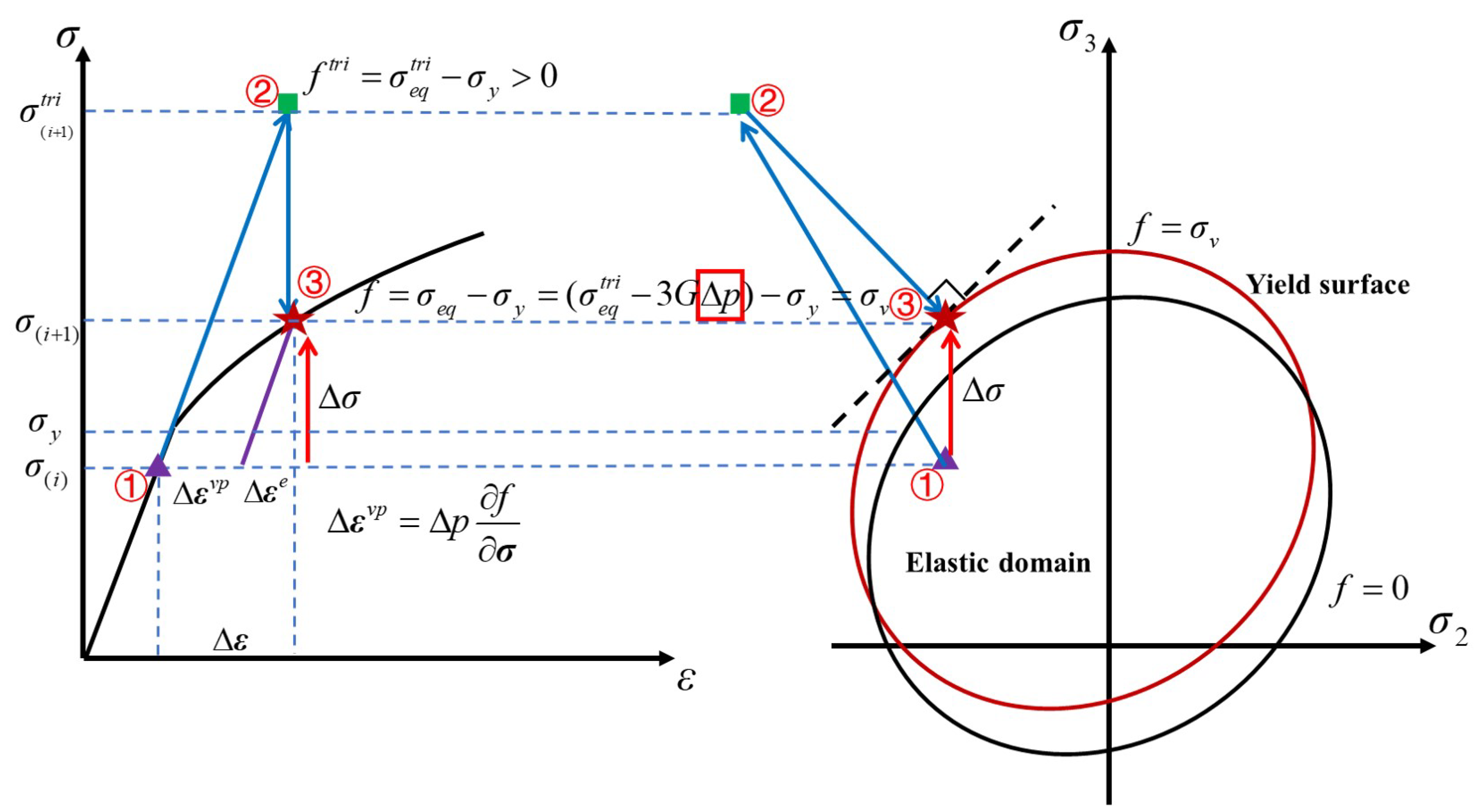
Figure 1. The stress-strain update process based on return mapping algorithm, and the corresponding yield surface.

Figure 2. Flow diagram of return mapping algorithm.

Figure 3. 316 Stainless Steel specimen and finite element model: (a) 316 Stainless Steel specimen[18], (b) uniaxial loading boundary condition, (c) meshing model.

Figure 4. Comparison of 316 Stainless Steel experimental and numerical results at room temperature: (a) uniaxial tensile stress-strain curves for different strain rates, (b) stress relaxation curve.

Figure 5. Comparison of model predictions of cyclic hardening behavior of 316 Stainless Steel with experimental data at 550°C: (a) stress-strain loops of the 1st cycle and the 50th cycle, (b) half stress range(

Δ σ / 2

)-cycle number(N) curve.

Δ σ / 2

)-cycle number(N) curve.

Figure 6. Zircaloy-4 specimen and finite element model: (a) Zircaloy-4 specimen and loading system[25,28], (b) boundary condition for uniaxial loading in the z-direction, (c) meshing model, (d) boundary condition for uniaxial creep in the z-direction, (e) boundary condition for uniaxial creep in the y-direction.

Figure 7. Uniaxial tensile stress-strain curves of CWSR state and R state Zircaloy-4 for different strain rates.

Figure 8. Incremental uniaxial creep curves for z-direction and y-direction loading: (a) R state, (b) CWSR state.

Table 1. Material constants for 316 Stainless Steel at room temperature and 550°C[16,18].

$T (° C)$	$E (G P a)$	$ν$	$σ_{y} (M P a)$	b	$Q (M P a)$	$a_{1} (M P a)$	$C_{1}$	$a_{2}$	$C_{2}$	$K (M P a \cdot s^{1 / n})$	n
]1RT	185	0.3	82	8	60	58	2800	270	25	151	24
]1*550	141.26	0.3	31	31	27.8	86.3	6939	114.8	957.69	173	10

* RT means room temperature.

Table 2. Material constants for Zircaloy-4 at 350°C[28].

Recrystallized Zircaloy-4	Cold worked stress relieved Zircaloy-4
$E = 78000 M P a, ν = 0.4$	$E = 73000 M P a, ν = 0.42$
$N = 6.5 M P a, k = 2.4, {\dot{ε}}_{0} = 6.58 \times 10^{- 8} s^{- 1}$	$N = 15 M P a, k = 2.4, {\dot{ε}}_{0} = 1.5 \times 10^{- 6} s^{- 1}$
$q = 8000, q_{1} = 600, q_{2} = 65$	$q = 9000, q_{1} = 400, q_{2} = 10$
$r_{m} = 2.4 \times 10^{- 12} M P a \cdot s^{- 1}$	$r_{m} = 1.53 \times 10^{- 8} M P a \cdot s^{- 1}, r_{m 1} = 1 \times 10^{- 43} M P a \cdot s^{- 1}$
$α_{0} = 10 M P a, m_{0} = 8$	$α_{0} = 10 M P a, m_{0} = 2.7, m_{1} = 28$
$Y_{0} = 69 M P a, Y_{θ}^{s a t} = 13 M P a$	$Y_{0} = 177 M P a, Y_{i s o}^{s a t} = - 40 M P a, Y_{θ}^{s a t} = 30 M P a$
$b_{θ} = 35$	$b_{i s o} = 2.5, b_{θ} = 5$
$M_{11} = 0.398, M_{22} = 0.62, M_{33} = 0.666$	$M_{11} = 1.1, M_{22} = 1.2, M_{33} = 0.666$
$M_{13} = - 0.222, M_{23} = - 0.444, M_{12} = - 0.176$	$M_{13} = - 0.28, M_{23} = - 0.38, M_{12} = - 0.82$
$M_{44} = M_{55} = M_{66} = 3.8$	$M_{44} = M_{55} = M_{66} = 3.4$
$N_{11} = 1.038, N_{22} = 0.72, N_{33} = 0.666$	$N_{11} = 0.699, N_{22} = 0.562, N_{33} = 0.666$
$N_{13} = - 0.492, N_{23} = - 0.174, N_{12} = - 0.546$	$N_{13} = - 0.401, N_{23} = - 0.265, N_{12} = - 0.297$
$N_{44} = N_{55} = N_{66} = 0.295$	$N_{44} = N_{55} = N_{66} = 0.33$
$Q_{11} = Q_{22} = Q_{33} = 0.666$	$Q_{11} = Q_{22} = Q_{33} = 0.666$
$Q_{44} = Q_{55} = Q_{66} = 1$	$Q_{44} = Q_{55} = Q_{66} = 1$
$Q_{13} = Q_{23} = Q_{12} = - 0.333$	$Q_{13} = Q_{23} = Q_{12} = - 0.333$
$R_{11} = 0.303, R_{22} = 0.637, R_{33} = 0.666$	$R_{11} = 0.626, R_{22} = 0.88, R_{33} = 0.666$
$R_{13} = - 0.166, R_{23} = - 0.5, R_{12} = - 0.137$	$R_{13} = - 0.206, R_{23} = - 0.46, R_{12} = - 0.42$
$R_{44} = R_{55} = R_{66} = 2.07$	$R_{44} = R_{55} = R_{66} = 2.75$

Disclaimer/Publisher’s Note: The statements, opinions and data contained in all publications are solely those of the individual author(s) and contributor(s) and not of MDPI and/or the editor(s). MDPI and/or the editor(s) disclaim responsibility for any injury to people or property resulting from any ideas, methods, instructions or products referred to in the content.

© 2023 by the authors. Licensee MDPI, Basel, Switzerland. This article is an open access article distributed under the terms and conditions of the Creative Commons Attribution (CC BY) license (http://creativecommons.org/licenses/by/4.0/).

Copyright: This open access article is published under a Creative Commons CC BY 4.0 license, which permit the free download, distribution, and reuse, provided that the author and preprint are cited in any reuse.

MDPI Initiatives

Important Links

Choose an area of interest and we will send you notifications of new preprints at your preferred frequency.

Disclaimer

Implementation of ABAQUS User Subroutines for Viscoplasticity of 316 Stainless Steel and Zircaloy-4

Abstract

1. Introduction

2. Viscoplastic Constitutive Equation

2.1. The Framework of Unified Viscoplastic Constitutive Model

2.2. Isotropic Viscoplastic Constitutive Model for 316 Stainless Steel

2.3. Anisotropic Viscoplastic Constitutive Model for Zircaloy-4

3. Computational Algorithm

3.1. Return Mapping Algorithm

3.2. Stress Update Algorithm of 316 Stainless Steel Model

3.3. Stress Update Algorithm of Zircaloy-4 Model

4. Verification and Validation of FE Modeling and UMAT Code

4.1. 316 Stainless Steel

4.2. Zircaloy-4

5. Conclusions

Author Contributions

Data Availability Statement

Acknowledgments

Conflicts of Interest

References

MDPI Initiatives

Important Links

Subscribe