1. Introduction
The samples were manufactured from PLA (Polylactic Acid), which is widely used to produce complex components made from polymer materials. PLA is a popular choice in additive manufacturing due to its biodegradability, ease of processing, and reasonable costs. PLA has its own limitations in terms of surface finish, dimensional accuracy and overall quality of the complex parts made by 3D printing. Through the proposed hybrid manufacturing approach, the combination of FDM printing with a milling operation, the researchers aim to address these limitations and improve the surface quality and dimensional accuracy of the PLA-based parts.
Additive manufacturing operations such as fuse deposition modeling (FDM) are frequently used for modeling, small application batches, and realizing small to medium prototypes. Being a manufacturing operation with a smaller cost compared to the other options, this will be used more frequently for obtaining 3D-printed parts. It is well known that the accuracy and the surface finish of the 3D printed parts are not the greatest, but these results to some extents are correlated with the printing parameters. In the cases in which the obtained result is not the desired one, although the input parameters were chosen based on some studies or on experience, additional operations need to be performed. Operations like milling a 3D printed part can highly improve the roughness and the accuracy of the final part. Thereby hybrid manufacturing concept is introduced. Both technologies have their own limitations. The milling process has limitations related to complexity, making milling not suitable for producing complex shapes or internal features. The complexity of the part is limited by the size of the cutting tool, which can result in additional processes to complete the part. Milling is not suitable for all types of materials, especially those that are soft or brittle, as they can easily deform or break under the pressure of the cutting tool. Being an expensive process, as it requires specialized equipment and skilled operators.
On the other hand, FDM printing has limitations on the resolution of the parts it can produce. The quality of the final product can be limited by the layer height and the accuracy of the printer.
Despite these limitations, milling and FDM printing are still valuable manufacturing techniques, as they offer unique advantages that other techniques do not provide. It is important to choose the right technique based on the specific requirements of the application.
2. State of the art
HM technology has witnessed remarkable advancements in recent years but at the same time with a drawback package that came. The aspects related to the drawbacks of both techniques can be minimized by combining both technologies [
1,
2]. A.N.M. Amanullah in [
3] designed and manufactured a similar type of equipment able to perform printing and milling operations on the same structure. The innovation was installing the CNC cutting spindle and the heated extruder of the FDM on a rotary structure and using the infrared sensors (IR) which simplified the mechanism structure and overcomes the problem with misalignment of the manufacturing tools.
The incorporation of five axes in this machine brings several benefits, which were showcased [
4]. For instance, the five-axis machine successfully created overhang features without the need for support material. This not only reduced costs and build time associated with support but also minimized the risk of deformation caused by support material removal. Moreover, the five-axis hybrid system enabled the production of FDM parts with embedded material, a task that cannot be achieved on a standard three-axis FDM machine. The inclusion of embedded material effectively enhanced the stiffness of the FDM item while reducing manufacturing time and costs. Furthermore, strategic use of the embedded material could improve stability by lowering the center of gravity of the FDM part. The hybrid system also demonstrated its capability to trim freeform surfaces and enlarge tapered holes in FDM parts, which cannot be accomplished using traditional three-axis RP machines. Notably, the hybrid technique significantly reduced build time by 44% and 58% in two specific cases. The advantages offered by the proposed hybrid system, combining FDM and five-axis machining, were evident and impactful.
In terms of surface quality, the Ra parameter, used as an indicator in this study [
5], shows superior performance at lower feed rates (400 mm/min) and a low depth cut (0.2 mm) across all studied rotational speeds. On the other hand, when considering burr height, the minimum heights are achieved by employing a higher feed rate (800 mm/min), a higher level of depth cut (0.8 mm), and a relatively high rotational speed. This phenomenon can be attributed to the heat exchange during the milling process. As the tool remains in contact with the sample surface for a longer duration, it leads to an increase in temperature and subsequently an increase in burr height. Furthermore, the optimal milling parameters for achieving better surface quality differ from those that result in lower burr formation. It was discovered that when pooling was not used, only the thickness of each layer had a significant effect of 49.37% at a 95% confidence level. However, when pooling was employed, the layer thickness had an increased effectiveness of 51.57% at a 99% confidence level. Additionally, the factors of material width and printing speed contributed significantly, accounting for 15.57% and 15.83% respectively, at a 99% confidence level. The correlation analysis further emphasized the importance of layer thickness, demonstrating a strong inverse relationship with surface roughness.
Based on the SIN analysis, it was determined that the layer thickness had the greatest impact when set at level 3 (0.3556 mm), while the road width was most effective at level 1 (0.537 mm), and the deposition speed at level 3 (200 mm). Bintara R. in [
6] studied and examined the surface roughness and production duration as key parameters. The analysis revealed that the layer height plays a significant role in determining surface roughness. The smallest roughness was observed at a layer height of 0.05 mm, while the lowest roughness occurred at a layer height of 0.25 mm. Furthermore, optimal printing parameters were identified at layer heights of 0.15 mm and 0.2 mm.
Based on the research conducted by Pamarac R in [
7] it was identified the optimal parameters for milling 3D printed components while maintaining a consistent spindle speed of 3500 revolutions per minute. In the case of PLA, a higher cutting speed leads to improved surface quality. This distinction arises from the fact that PLA has a lower melting temperature. Consequently, the longer the cutting tool remains in contact with the component, the more heat is generated, resulting in a degradation of the part's surface. In another article [
8] the researchers aimed to study the behavior and the roughness of the surface also including the printing angle. It was found that a measuring direction of 90° yielded the most representative value for the distribution of surface roughness (Ra), compared to measuring angles of 0° and 45°.decreasing the nozzle diameter from 0.3 mm to 0.2 mm and reducing the layer height to 0.1 mm resulted in a significant increase in both the build time and the consumption of thermoplastic filament for printed parts number 5 and number 6. In terms of the inner faces of the printed parts, the highest surface roughness behavior was observed at 45° measuring direction, with a value of 36.96±0.51 µm, while the lowest surface roughness behavior was recorded at 0° measuring direction, with a value of 1.35±0.27 µm. These measurements were obtained using a nozzle diameter of 0.5 mm and a layer height of 0.3 mm.
For the outer faces, the highest surface roughness behavior was measured at a 45° measuring direction, with a value of 34.94±1.04 µm, using a nozzle diameter of 0.5 mm and a layer height of 0.3 mm. Conversely, the lowest surface roughness behavior was found at a 0° measuring direction, with a value of 1.08±0.30 µm, using a nozzle diameter of 0.3 mm and a layer height of 0.2 mm. Comparing the inner and outer faces of all six configurations of FDM 3D printed parts, it was observed that the surface roughness behavior differed by approximately 2 µm (5%) for higher values. Conversely, for lower values of surface roughness behavior, the difference between the inner and outer faces was approximately 0.27 µm (20%).
In another study [
9] the impact of technological parameters on surface roughness, material deposition, and hybrid manufacturing time was investigated using a statistical approach. Regression models were analyzed to determine the optimal values for parameters such as spindle speed, layer height, material compensation flow, printing speed, feed speed of the milling tool, and milling depth. The findings showed that layer height had the most significant influence on surface roughness, with higher layers resulting in minimal roughness. The material compensation flow had no effect on roughness at the highest layer height. A high spindle speed could cause material winding on the tool's surface, so a lower value was deemed optimal. The feed speed of the milling tool had an inverse relationship with roughness. The impact of milling depth varied depending on the nozzle size. The material deposition was primarily influenced by the material compensation flow, while hybrid manufacturing time was minimized by using the fastest printing speed and highest layer height. In conclusion, using a larger nozzle size allowed for achieving the same final surface roughness as the smaller nozzle size but with significantly higher productivity. his research aimed to investigate the surface roughness of 3D printed parts manufactured using a low-cost desktop FDM 3D printer and PLA+ thermoplastic filament.
In another study [
10] the researchers were using neural model optimization to predict surface roughness and it was observed that the Artificial Neural Network models exhibited greater accuracy in predicting surface roughness. By analyzing the Root Mean Square Error and Mean Absolute Percentage Error values, it was evident that the neural model Multilayer Perceptron (MLP) 4-15-1, incorporating four input variables (three cutting parameters and machining vibration), displayed a higher average prediction accuracy of 93.14% compared to the model MLP 3-13-1, which only considered three cutting parameters. These findings provide clear evidence that incorporating spindle vibration into the prediction algorithm can enhance the accuracy of predictions. D. Kramar in [
11] used regression models to identify the optimal values for various parameters, including spindle speed (n), layer height (h), material compensation flow (Φ), printing speed (v), feed speed of the milling tool (vf), and milling depth (ap). Regarding surface roughness, the primary factor influencing roughness was found to be the layer height (h). Achieving the highest layer height resulted in minimal roughness (Ra and Ry) when measuring in different directions. At this specific layer height, the material compensation flow (Φ) was observed to have no significant impact on roughness. Additionally, a higher spindle speed (n) was found to lead to material winding on the tool's surface, so a lower value was considered optimal. The feed speed of the milling tool (vf) exhibited an inverse relationship with roughness. The depth of milling (ap) had only a marginal influence, with a smaller milling depth contributing to better roughness when using a smaller nozzle size while having a minimal impact with a larger nozzle size. In terms of material deposition during hybrid manufacturing, the primary factor influencing deposition (MD) was found to be the material compensation flow (Φ), which had a proportional effect.
3. Mathematical modeling by linear regression of printing and milling
For a better understanding of the process,
Figure 1 and
Figure 2. is presented a workflow that represents the steps performed during this research to find and optimize the manufacturing parameters for milling and printing operation.
The parameters that were chosen to be studied and collect data from them were chosen based on preliminary experiments performed on separate printing and milling equipment, experience, and other studies [
11].
Data collection for the milling operation included preliminary experiments using the following input parameters:
Data collection for the printing operation included preliminary experiments having the following input parameters:
While printing the samples a standard nozzle of 0.5 mm was used and for the milling tool, it was used an HSS milling tool of 6 mm diameter with 4 teeth.
As the focus of the study was by having the controllable factors in our case the milling and the printing parameters to establish optimize and predict the uncontrollable factors also called noise factors like roughness. The technological parameters were examined on three levels -1 is the lowest value of the parameter, +1 is the highest value of the examination parameters, and 0 represents the average between the low -1 and the high +1.
Table 1.
List of technological parameters on 3 levels.
Table 1.
List of technological parameters on 3 levels.
| Level |
n [rot/min] |
vf [mm/min] |
ap [mm] |
v [mm/s] |
h [mm] |
Φ [%] |
| -1 |
500 |
80 |
0.1 |
30 |
0.2 |
80 |
| 0 |
5250 |
240 |
0.2 |
55 |
0.26 |
90 |
| 1 |
10000 |
400 |
0.3 |
80 |
0.32 |
100 |
The analysis for optimizing the manufacturing parameters was taken separately for the printing operation as well as for the milling operation, in order to be studied individually. The Taguchi L16 method is used to efficiently identify the optimal combination of parameter settings in hybrid manufacturing by conducting a limited number of experiments, analyzing factor interactions, and improving product quality by minimizing surface roughness. The decreased number of preliminary experiments, both for printing and milling, in order to select the relevant necessary experiment are presented in
Table 2 and
Table 3.
The output parameter Ra [µm] represents the roughness values required for the model validation and represents the measurement value for each experimental set. The roughness measurements were performed with a Mitutoyo Contracer CP - 200 / 400 - Contour Measuring Instrument.
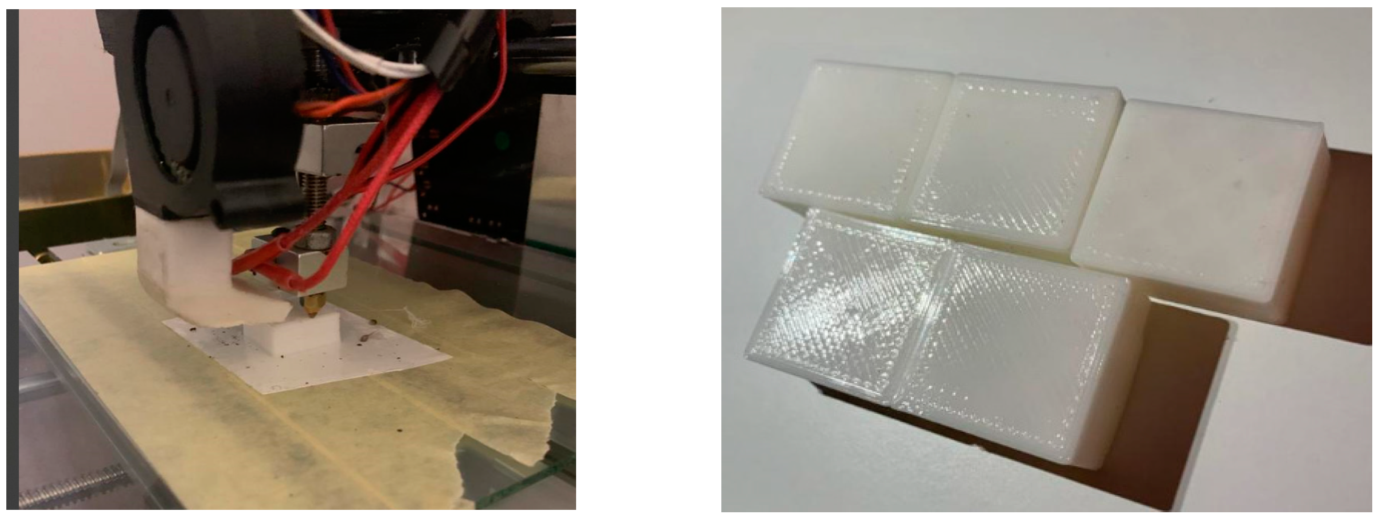
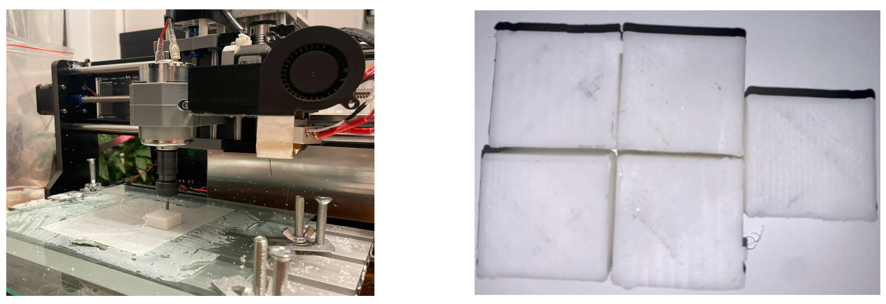
In
Figure 3 and
Figure 4 are illustrating the hybrid prototype engaged in the printing and milling operation. The new HME prototype design by the author requires specific sets of parameters both for milling and printing which depends on specific components of the HME which had a special calibration procedure. That is why process parameter optimization is required to provide the best surface quality and to reduce material consumption.
3.1. Data Analysis and Model Generation
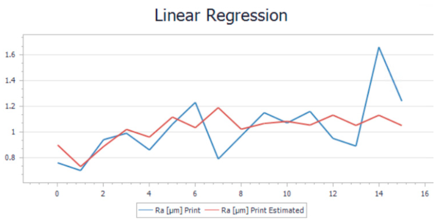
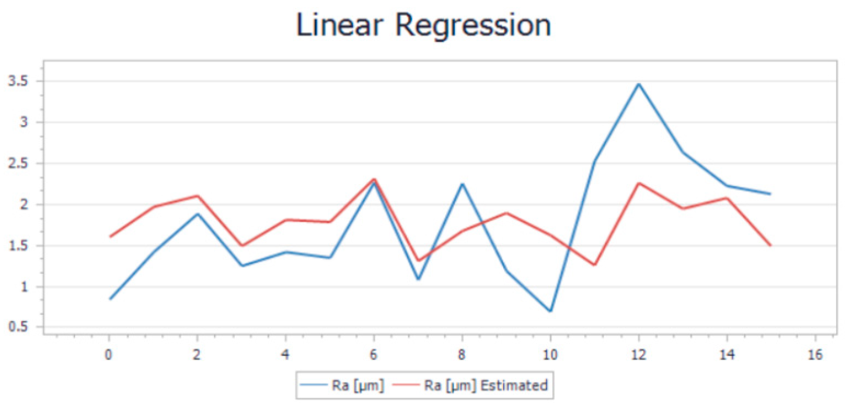
After performing all 32 experiments on the hybrid, and all the necessary output data was collected, the values were uploaded into Project Modeling 5.3 Software for further analysis. After the data was imported, the first step was to trend the whole batch of data. This action was required in order to see if there were any anomalies that could affect the model. This step of cleaning the data is a step necessary before running the model algorithm. Once the cleaning operation was performed, the data is imported into a Linear Regression Model (LRM) to be analyzed. The goal of linear regression is to find the best linear relationship between the variables that minimize the sum of squared errors. The results of the model are illustrated in
Figure 5 for the printing operation and in
Figure 6 for the milling operation. For a more visual understanding of the results, a trend representation was made with the actual roughness of the sample and the estimated roughness of the model for both cases.
As can be observed from both trends there is a slight variation in the trends when comparing the measurement roughness and the estimated one. The mathematical formulas of both models were generated by the software application based on the input and output parameters. The Ra estimate was generated by applying in the formula the input parameters. Eq.1 represents the mathematical model used to determine the roughness obtained for the printing operation while eq.2 represents the mathematical model used in the determination of the roughness for milling. These equations can estimate the final roughness of the part when requirements or limitations like the rotation of the spindle are involved.
By analyzing the accuracy of the model, the value of the average relative error was 0.13% for printing and 0.38% for milling. Theoretically, it is considered of being too high and whose value needs to be as close as possible to 0. Another important indicator was the F-test which measured if the overall regression model is statically significant. A high F-statistic and a low p-value indicate that the model is a good fit for the data and that the independent variables included in the model are significant predictors of the dependent variable. In our case, the F-statistic and p-value for printing are 1.20% and 0.349%. The same indicators for milling are 0.48% and 0.85%. R-squared indicator whose value needs to be as close as possible to 1 and in this case, it has values around 0.13-0.38%. These indicators presented are showing that the model may be considered moderately accurate, but not highly accurate. The average relative error of 0.38% and 0.13% indicates that, on average, the model's predictions are off by about 31% respectively 13% from the actual values. This means that the model's predictions may have a significant margin of error, which could limit its usefulness.
- a.
Model Validation
To perform a validation of the mathematical model for both operations a workflow diagram it was established in
Figure 7 for the operation process and
Figure 8 for the milling operation.
In practice, the user knows the required surface quality of the part which has to be obtained and needs to set up the optimal parameters of the HME in order to obtain the part with surface quality. Starting from the input and output values presented in
Table 2 and
Table 3 it was generated in Project Modeling Studio Software five sets of optimized parameters for each operation. The parameters are presented in
Table 4. These actions are required in order to validate our mathematical model. The next step of the validation process was to manufacture the samples accordingly to
Table 4 in which are both presented.
After manufacturing, a new set of roughness measurements are performed, and new data is obtained. In
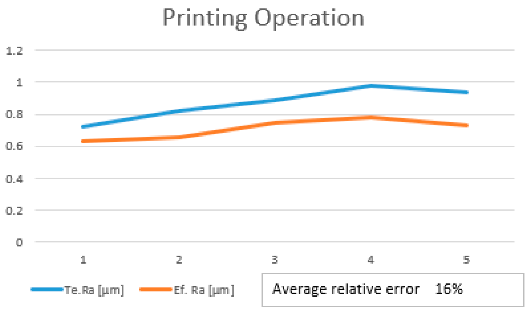
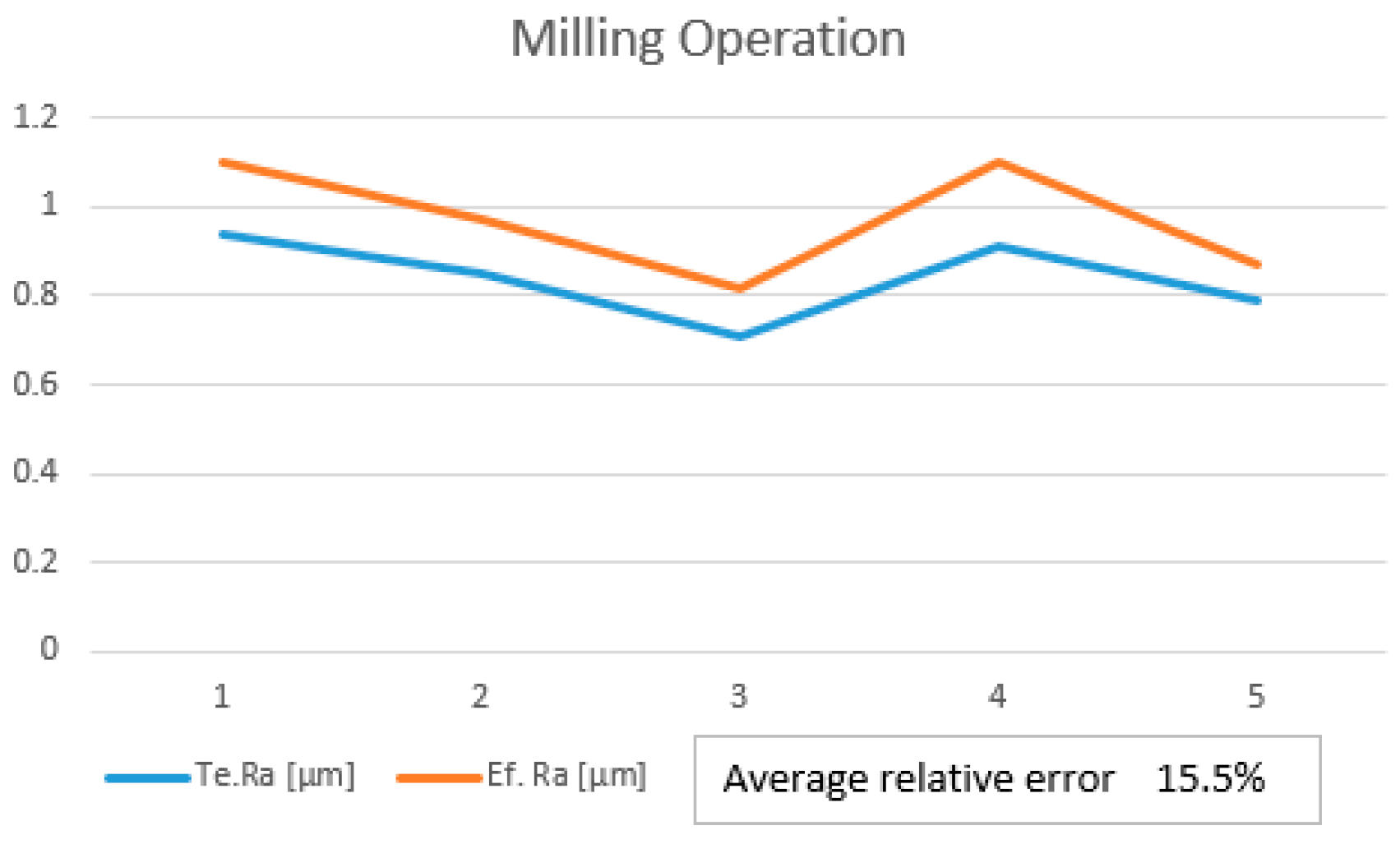
Table 4 Te.Ra is the theoretical value using Eq.1. And Eq.2. The final step was to perform the validation of the linear regression model using the optimized parameters. For this validation step, the values of the effective roughness were compared with the value of the theoretical roughness. By analyzing the roughness value, it can be seen that the value of the effective roughness decreased as compared to the previous values before optimization. The optimization was based on choosing to modify the correlated inputs which are influencing the manufacturing operations. Because none of the input parameters were highly correlated with the roughness, all the parameters were taken in the analysis for improvements in the model performance. To provide a better understanding of the small differences between theoretical roughness Te.Ra and the effective roughness Ef.Ra a trend using their values was provided. In
Figure 9 is presented the validation trend for printing operations. It can be seen that the average relative error of the model is 18.1%. In Figure10 is presented the validation trend for milling operations and also in this case the measured roughness was above the theoretical values.
The mathematical model has some small deviations from the effectively measured roughness. After conducting a comparative analysis of the theoretical roughness and effective roughness it was determined that the mean absolute error (MAE) between the predicted values and the actual values was 0.16/0.13 µm. This result may require further refinement to improve the accuracy.
4. Neural network modeling to improve the linear regression model
Starting from the assumption that the linear regression model of this study can be further optimized, the same batch of samples will be used for building the model. The neural network model is a more complex and flexible method that can capture non-linear relationships between variables. It involves a network of interconnected nodes that process and transmit information. The Levenberg-Marquardt algorithm was used as an optimization algorithm. This algorithm is one of the methods used for training a Neural Network model, which involves adjusting the weights between the nodes to minimize the error between the predicted and actual values. By maximizing the power of neural networks and by using the Levenberg-Marquardt algorithm, you can use complex patterns could be modeled and more accurate predictions could be obtained from the available data. This approach is particularly valuable when dealing with small datasets where linear regression may not adequately capture the underlying relationships between variables.
The input and output data were imported again into the Project Modeling Studio Software. One of the most important parameters for this method used to generate an accurate model is the iterations, learning rate, and hidden layers in the network. The iterations refer to the number of times the optimization algorithm updates the weights and biases of the network in order to minimize the loss function. The optimization process involved an iterative approach to adjusting the weights and biases of the neural network to minimize the loss function. The loss function measures the difference between the predicted output of the neural network and the true output. The goal is to minimize this difference by iteratively adjusting the weights and biases of the network. The total number of iterations was considered 5000. The learning rate is the training parameter that controls the size of weight and bias changes during the learning process. The value of this parameter was selected as 0.1. The hidden layers are layers of artificial neurons that are located between the input layer and the output layer. The term hidden refers to the fact that the operations performed by the neurons in these layers are not directly visible or accessible from outside the network. The input layer of a neural network receives the input data, which is then processed by the hidden layers before being passed to the output layer. Each neuron in a hidden layer receives input from the neurons in the previous layer, applies a mathematical function to the inputs, and produces an output that is passed on to the next layer. The value of this parameter was set to 2. For both neutral network models that will be analyzed the settings used were the same, just the input parameters were different. Once the neutral network models are generated, the results can be analyzed in the sections below.
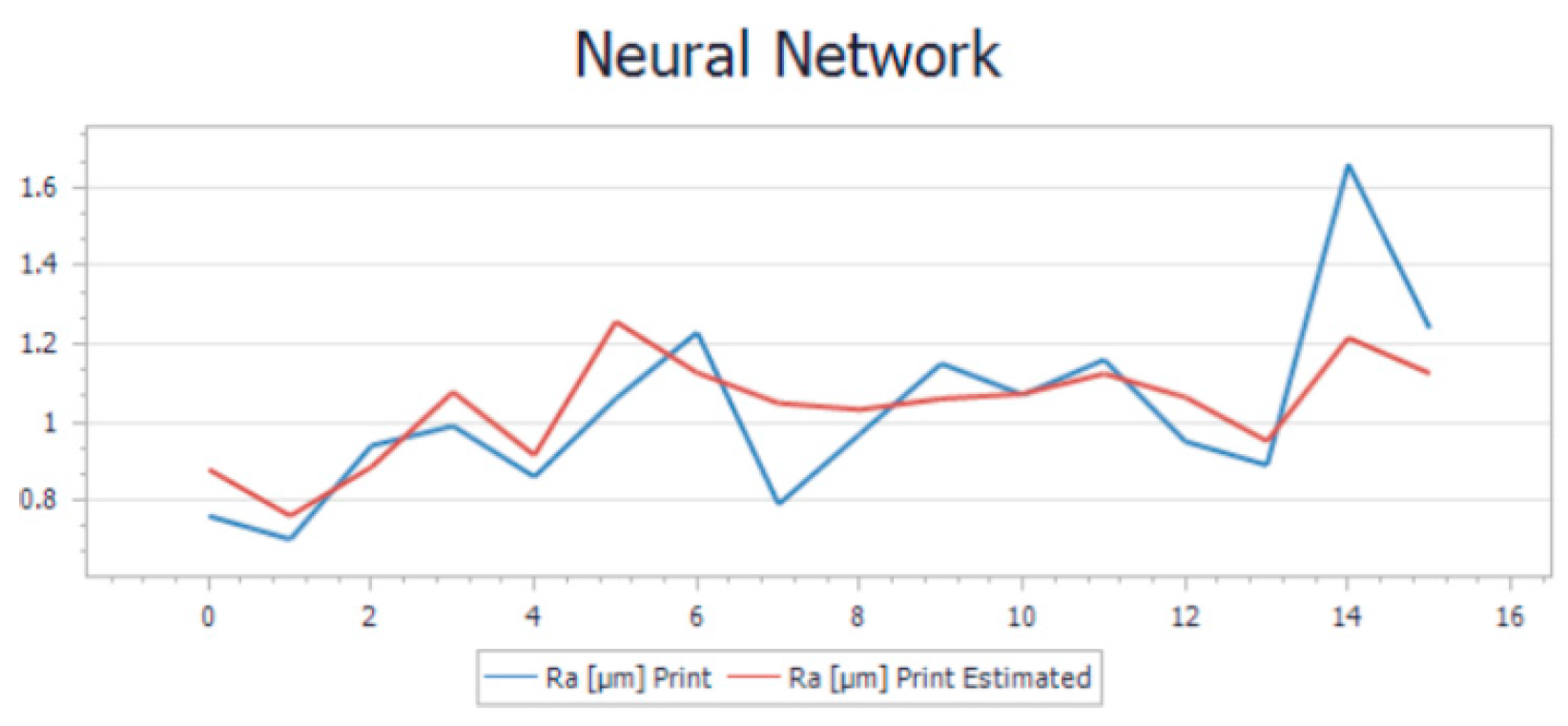
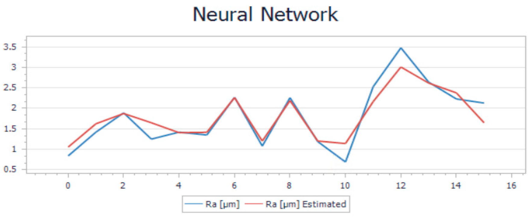
The trend of the new model that is presented in
Figure 11 and
Figure 12 represents the overlapping onto the same graphic of the estimated and the calculated roughness. Based on the R-squared and average relative error values, it seems that the model is performing well. An R-squared value of 0.4% and 0.8% indicates that the model can explain a significant portion of the variance in the target variable, which is a positive sign. Additionally, an average relative error of 0.11% and 0.13% suggests that, on average, the model's predictions are relatively close to the actual values, which is also a good sign.
The end scope of the neural network model was to generate and export a DLL model. The dynamic link library (DLL) is a type of file that contains reusable code and resources that can be used in other programs. For our case, the DLL is needed to create a software application that is able to predict the final roughness of the part.
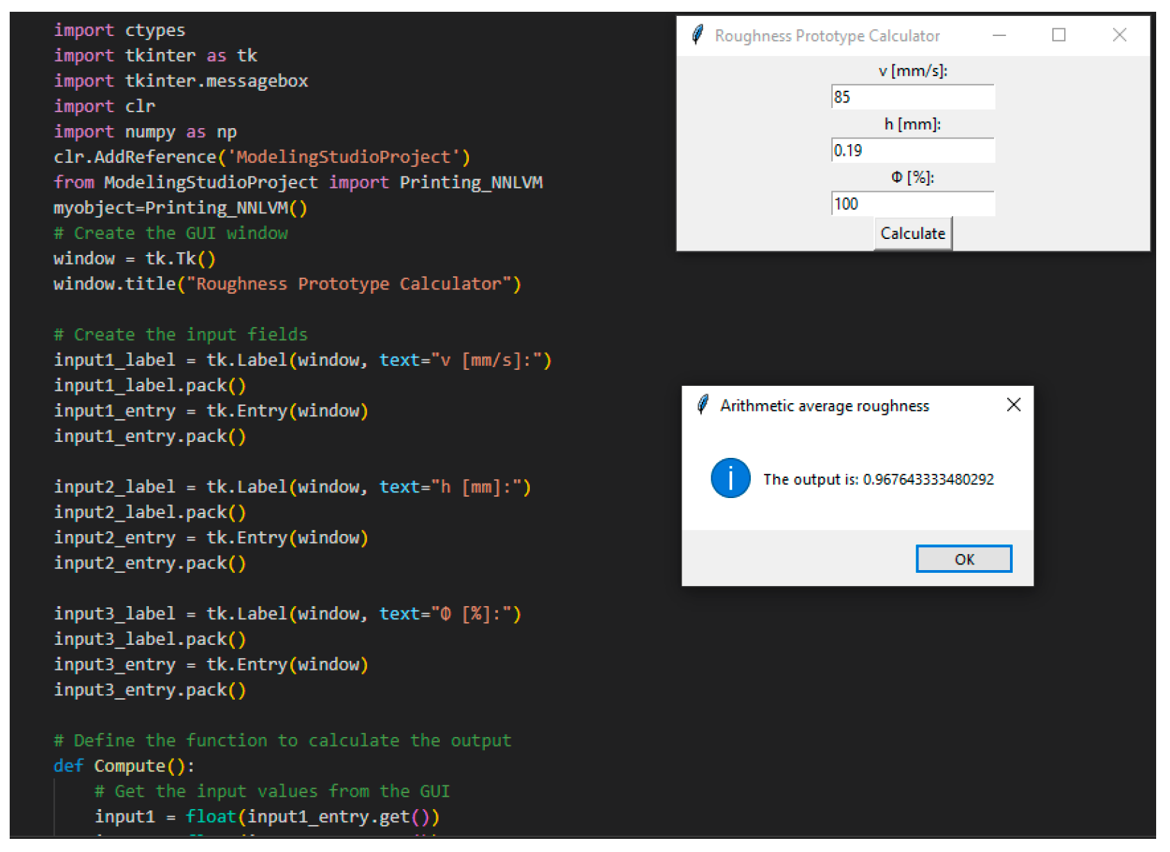
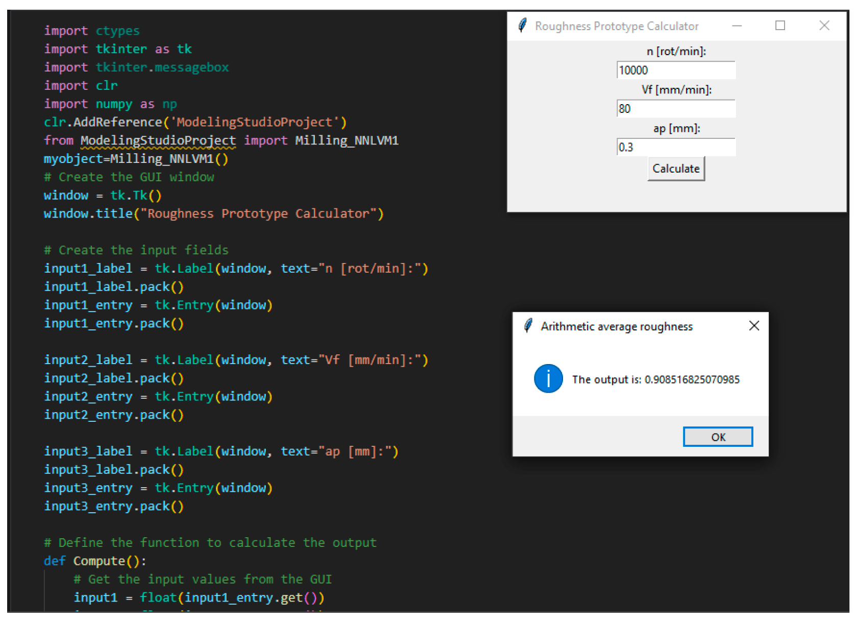
The code for the new application was written in Python and in
Figure 13 and
Figure 14 are presented the Graphical User Interface (GUI) of the application. The application is called Roughness Prototype Calculator. The application can be used for both manufacturing processes of milling and printing. The whole Python program written for this neural modeling is presented in Anex1.
The new theoretical values of the roughness estimated by the new NNM, are presented in
Table 5. A comprehensive comparison was conducted between the roughness values obtained from the linear regression model (LRM), neural network model (NNM), and the actual R
a measurements of the test samples.
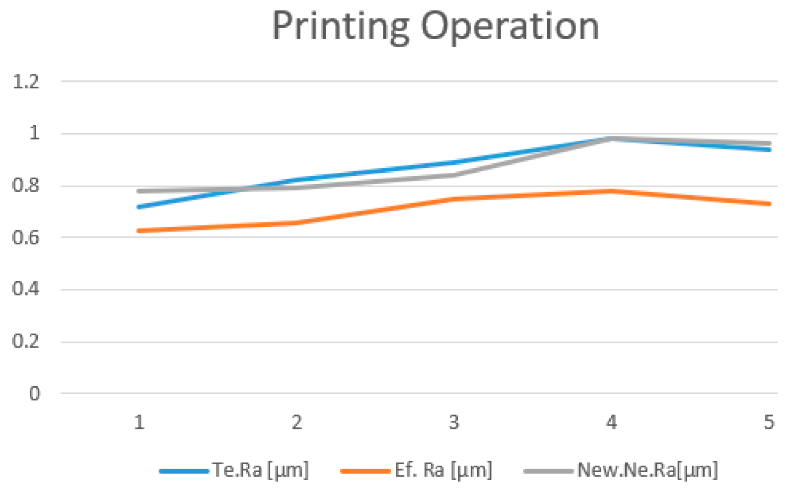
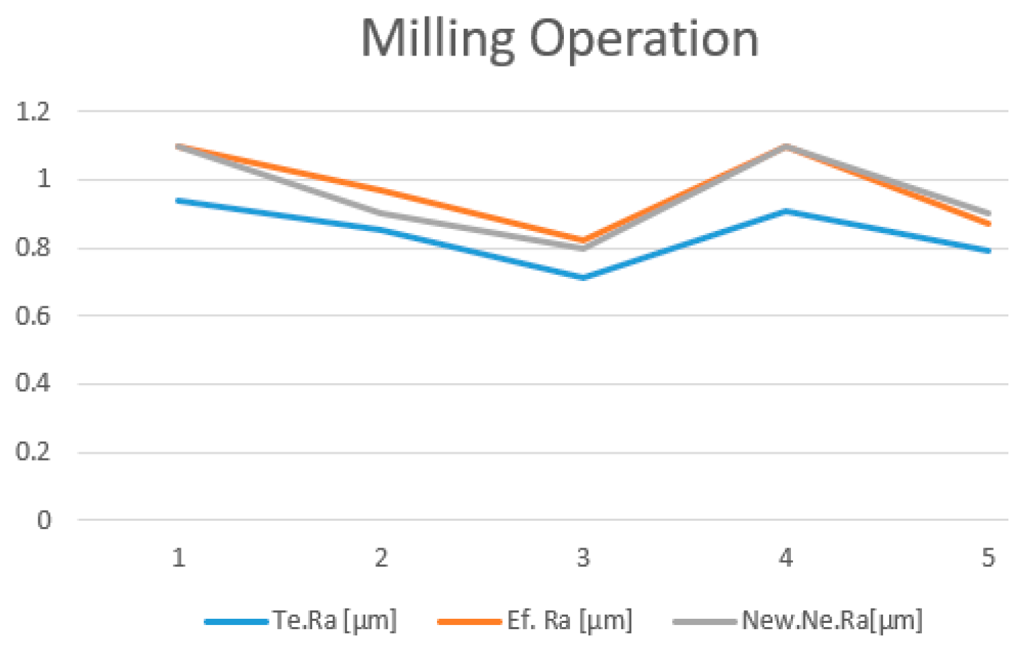
The visualization trend of the comparison between the results generated by the two models and the measured roughness is illustrated in
Figure 15 and
Figure 16.
The validation of the new NNM modeling was done by using the same set of experimental data presented in table 4, both for printing and milling. Besides the estimated values obtained by LRM, table 5 presents also the estimated values obtained by NNM and the predictions from both modeling methods have been compared to the values measured on the probes.
Analyzing all the aspects presented and also comparing the two models, we considered that for this particular case, the most suitable solution is to use the Neural Network Model for optimization and prediction of the surface roughness.
5. Experimental research to test the new process parameters, optimized for HME
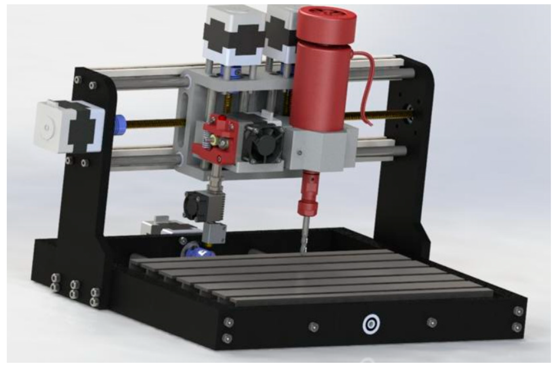
The HME Prototype illustrated in
Figure 17 was designed and manufactured by the authors. That is why proper calibration and optimization of the process parameters was essential, to get the most of this new hybrid equipment.
The whole optimization methodology presented in this paper could be applied for other prototypes, in order to find their optimal process parameters.
The hybrid manufacturing equipment prototype was used for this research. The prototype combines the printing operation with milling, as shown in
Figure 17. The HME Equipment illustrated in
Figure 17, was designed and manufactured by the authors, Details about the constructions and characteristics of this equipment have been published in the article [
13]. The main characteristics of this new hybrid equipment are presented below. The main structure of the HME was the one of a Mini CNC equipment and FDM 3D printing head. Precise and accurate operation is of utmost importance for this particular type of equipment, as it guarantees that the manufactured parts meet specific dimensional requirements and align with the original design consistently. The equipment must possess the capability to produce parts with tolerances as low as 0.1 mm, necessitating precise control and movement of the materials involved. The primary advantages lie in its speed and efficiency, enabling the production of parts quickly and efficiently without compromising on quality. This necessitates high-speed printing mechanisms capable of generating multiple material layers in a short timeframe, while effectively managing substantial volumes of diverse materials.
Material compatibility represents another vital requirement, as the equipment should be able to work with a wide range of materials, allowing for versatility and adaptability to meet the specific needs of various projects. Customization is also crucial, allowing for the production of parts and objects with unique shapes, sizes, and features. To achieve this, the equipment must be adaptable to different design requirements and be able to employ various processes and techniques. User-friendliness is an essential aspect of this equipment, particularly considering that it should be easy to use even for individuals with limited or no prior experience in manufacturing. Furthermore, it should require low maintenance and easily replaceable parts to minimize downtime and maximize efficiency.
Moreover, the equipment's final design must be cost-effective, affordable, and capable of producing parts and objects at a high rate without compromising on quality or accuracy. This ensures that it can be utilized for both prototyping and manufacturing purposes, serving as a cost-effective solution for companies of all sizes. One of the main challenges faced during the design of the new prototype was the integration of the milling equipment and the FDM extruder while keeping the assembly simple and avoiding excessive complexity. The solution was to combine both tools, the extruder, and the cutter spindle, on the same x-axis but with a 10 cm offset. The base of the equipment was positioned on the y-axis, while the z-axis was attached to the x-axis to control the layer height and cutting depth during the manufacturing process.
In addition to the x, y, and z-axis, two special axes, A and B, were added to guide the milling and printing tools. The x-axis had a total range of motion of 300 mm, with 250 mm being the active range. The y-axis had a total range of motion of 180 mm, with an active range of 150 mm. The z-axis had a total range of motion of 45 mm, with an active range of 30 mm. The overall dimensions of the equipment were 450 mm (width) x 280 mm (depth) x 360 mm (height). These dimensions were chosen to provide a stable and solid chassis, as milling processes involve greater forces compared to printing processes. The chassis used in this prototype was sourced from a Mini CNC equipment called VEVOR CNC 3018 Pro.
The next step involved designing a new set of supports to mount the manufacturing tools on the x-axis. SolidWorks software was utilized to obtain the CAD model for this purpose. The 3D printing operation was performed using a Prusa I3 3D printer. Once the supports were manufactured, they were used to hold the manufacturing tools, and the subassemblies were mounted on the guiding system. For this type of construction, it was necessary to have two motors on the z-axis to control the two manufacturing tools independently.
The FDM extruder subassembly used in this prototype was a low-cost one and consisted of several components, including a Nema 17 stepper motor, an extruder gear, a hot end, a nozzle, a filament drive, and a cooling system. The stepper motor drove the extruder gear, which pushed the filament through the nozzle. The extruder gear gripped the filament and pushed it through the hot end, where it was melted and extruded through the nozzle. The hot end included a heating element, a temperature sensor, and a cooling fan. The size of the nozzle played a significant role in the final surface finish and the overall print quality.
The filament drive system ensured a consistent flow of filament and comprised the extruder gear, a guide tube (PTFE tube), and a filament drive mechanism. A cooling system was employed to cool the filament after it was extruded, preventing deformation, and ensuring the printed object retained its shape.
The milling subassembly equipment included a spindle motor, a spindle housing, a tool holder, bearings, a cooling system, a drive system, and control electronics. The spindle motor was the main component responsible for rotating the cutting tool and performing the milling operation. It was a high-speed motor capable of reaching tens of thousands of RPMs.
To manage both the 3D printing and CNC milling processes, a sophisticated control system and software were required. The control system coordinated the operation of both processes, including the movements of the printer's motors and the operation of the extruder and milling head. The control system utilized an Arduino UNO R3 microcontroller board and a Shield V3 designed to control both CNC and 3D printing. The Shield included sockets for 5 A4988 stepper drivers and was powered separately. It also featured additional filtering capacitors for each driver to ensure precise equipment movements. Cura was used as the user interface software for generating G-Code in the printing process, providing settings for print material and quality parameters. Grbl Control software was used for controlling the CNC milling head, executing the G-code generated in Solid CAM. This software generated tool paths compatible with the printer's positioning system, enabling real-time execution.
The prototype also included an offline control module, allowing for equipment control through its own interface, as shown in
Figure 7. The G-code interpreter used was Merlin, which translated the G-code commands generated by the slicing software into appropriate motor control signals. The G-code interpreter handled complex instructions involving both 3D printing and milling. Regular firmware updates were considered important based on experience.
In addition to the control software for 3D printing, a separate software program was required to control the CNC milling head. This software was responsible for generating tool paths for the milling head to cut the part. It needed to generate tool paths compatible with the printer's positioning system and capable of real-time execution.
The prototype of the HME illustrated in
Figure 17 was manufactured and tested by the authors. This prototype of the new equipment needs to be calibrated and the process parameters, both for printing and milling, need to be optimized, in order to improve the surface quality and to reduce the material consumption. Usually for commercially available equipment the manufacturers do recommend the optimal process parameters for different materials.
When a new prototype is designed and manufactured a specific process optimization is required to improve the printing and milling output. That is why the aim of the research presented in this article is to optimize the process parameters and to calibrate and get professional results from this prototype.
The methodology presented in this article could be used by other researchers when a new manufacturing prototype is designed and manufactured.
Current testing methods for hybrid manufacturing equipment involve the usage of multiple parts to evaluate the different aspects of the system. For example, one test may focus on the dimension and geometrical tolerancing, and another test on surface quality on different surfaces. While these testing new methods can provide valuable insights, they can also be time-consuming and expensive. However, using multiple parts can introduce variability and uncertainty into the testing process, making it harder to draw final conclusions about the performance of the equipment. To find a solution to these limitations, there is a need for a new part that can meet all the criteria for testing and validating hybrid manufacturing equipment. This part would need to be versatile enough to test a wide range of materials and parameters. It will also need to be robust enough to withstand the rigors of testing over an extended period. The need for a new part to test and validate hybrid manufacturing equipment comes from a need and desire to improve the accuracy, efficiency, and cost-effectiveness of testing in this field. By developing a new part that can meet all the requirements for testing and validation, the researchers and users can speed up the process of the development of new hybrid manufacturing technologies and improve the performance of existing systems.
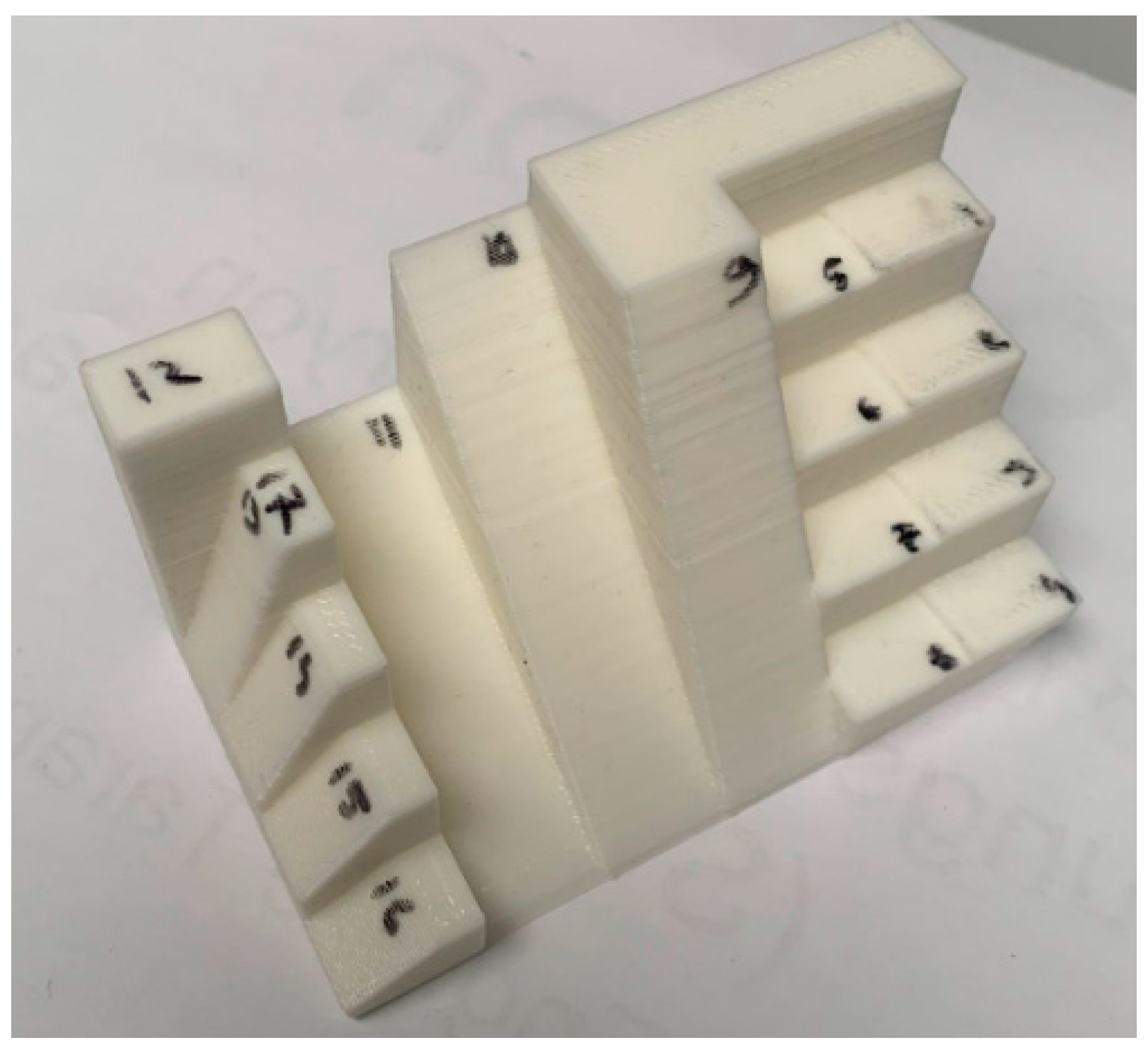
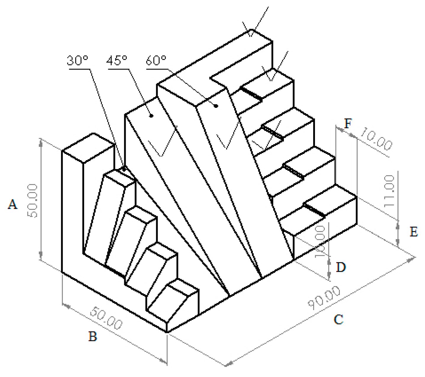
For this reason, in this chapter, it was aimed to extra validate the optimization parameters methods. A new part was designed and manufactured. The design of the part was realized in SolidWorks. The design of the part is illustrated in
Figure 18. The part is realized from PLM material. The equipment used to manufacture the part was the SP hybrid manufacturing prototype. The overall dimensions were measured with a caliper, and the roughness was measured with the same roughness measurement equipment as before. We design a new test part illustrated in
Figure 18, to be able to evaluate the performances of SP HME presented in
Figure 19. The test part for HME will be compared with the one from the technical drawing illustrated in
Figure 19. Each surface of the test part was numbered and both dimensional accuracy and surface roughness were measured against the process parameters obtained by the neural network modeling.
The specific test part illustrated in
Figure 18, and
Figure 19 were designed to test the capabilities of our new HME prototype. The optimization results obtained by using the presented mathematical modeling were applied and used for manufacturing these test parts in order to validate these sets of optimal parameters ( 5 sets generated by the software). In this manner the theoretical contributions brought by this article were tested on a practical complex test part illustrated in
Figure 18. And the values measured for the surface roughness were similar to the values measured on the 5 probes illustrated in
Figure 3 and
Figure 4.
The advantage resulting from using such a complex model to validate the hybrid equipment is the variety of measurements that need to be checked. The measurements that can be performed on this model are:
The results of the measurement are presented in
Table 5.
| Nr.crt. |
Targeted Value [mm] |
Measured Value [mm] |
| 1 |
0.9 |
0.83 |
| 2 |
0.9 |
0.89 |
| 3 |
0.9 |
0.81 |
| 4 |
0.9 |
0.81 |
| 5 |
0.65 |
0.62 |
| 6 |
0.65 |
0.65 |
| 7 |
0.65 |
0.74 |
| 8 |
0.65 |
0.73 |
| 9 |
0.65 |
1.13 |
| 10 |
0.65 |
1.49 |
| 11 |
0.65 |
2.43 |
| 12 |
0.65 |
0.66 |
| 13 |
0.65 |
1.5 |
| 14 |
0.65 |
1.26 |
| 15 |
0.65 |
1.30 |
| 16 |
0.65 |
1.19 |
| 17 |
50 |
49.5 |
| 18 |
50 |
49.8 |
| 19 |
90 |
90 |
| 20 |
10 |
10 |
| 21 |
11 |
10 |
| 22 |
10 |
10 |
In the first section of the table, the targeted values were set at 0.9 mm for entries 1 to 4, and 0.65 mm for entries 5 to 16. The measured values for these entries varied slightly around the targeted values, indicating a relatively close match between the targeted and actual measurements. However, there were some variations observed, especially for entries 9, 10, 11, and 14, where the measured values deviated significantly from the targeted values.
In the second section of the table, entries 17 and 18 had a targeted value of 50 mm, while entry 19 had a targeted value of 90 mm. For these entries, the measured values were very close to the targeted values, indicating a high level of accuracy in the measurements. Entry 20 had a targeted value of 10 mm, and the measured value matched precisely, indicating an accurate measurement. Entry 21 had a slight deviation, with a measured value of 10 mm instead of the targeted value of 11 mm. Entry 22 had both the targeted and measured values at 10 mm, indicating an accurate measurement.
In summary, the table demonstrates the comparison between targeted and measured values for a range of parameters or dimensions. While most measurements closely matched the targeted values, there were some instances of significant deviations, highlighting potential areas for further investigation or improvement in measurement accuracy.
6. Conclusions
Experimental research proved that polymer materials, such as PLA, are suitable for the hybrid manufacturing process, where the combination of 3D printing and milling operations led to improved surface roughness and a good accuracy of the PLA parts.
The undertaken case study for the complex test part made from PLA, proved the capability of our new hybrid manufacturing equipment and more important, this methodology could be replicated to optimize other similar artisanal hybrid manufacturing setups, to produce better components made from polymer materials.
The neural network model (NNM) produced more accurate results in predicting the final roughness (Ra), as compare to the linear regression model (LNM).
By using the optimized process parameters derived from the models, a good estimation of the obtained roughness (Ra) was achieved.
The deviation of the roughness (Ra) values from the predicted estimations was acceptable and remained relatively constant across all the samples tested.
The original approach of using neural network modeling (NNM) and developing specific Python programs to handle dynamic-link libraries (DLL) resulted in good outcomes for optimizing the usage of the new hybrid manufacturing equipment (HME).
The novelty of this research lies in the fact that even with a small number of experiments, accurate estimations can be obtained for the output parameters, specifically roughness (Ra) in this case.
Other users of new artisanal hybrid equipment can replicate this research methodology to enhance the functionality of their equipment by identifying their optimal process parameters, for a better functionality of their equipment.
Acknowledgments
This research was financially supported by the Project “Entrepreneurial competencies and excellence research in doctoral and postdoctoral programs -Antredoc”, a project co-founded by the European Social Found financing agreement no.56437/24.07.2019. This research was also supported by DiCoMI project Horizon 2020 (No 778068) (WWW.DicoMI.eu )
References
- Kozan, Ž. (2016), Optimization of the Technological Parameters in Hybrid Manufacturing. BSc thesis, University of Ljubljana, Faculty of Mechanical Engineering, Ljubljana.
- Sergiu Pascu1, Nicolae Balc1 and Adrian Augustin Pop2 2022, Reconstruction of Orbital Wall by Using Hybrid Manufacturing Operations, Dept. of Manufacturing Engineering.
- Amanullah, A., Murshiduzzaman, Saleh, T., & Khan, R. (2017). Design and Development of a Hybrid Machine Combining Rapid Prototyping and CNC Milling Operation. Procedia Engineering, 184, 163–170. [CrossRef]
- Lee, W. C., Wei, C. C., & Chung, S. C. (2014, November). Development of a hybrid rapid prototyping system using low-cost fused deposition modeling and five-axis machining. Journal of Materials Processing Technology, 214(11), 2366–2374. [CrossRef]
- Mehtedi, M. E., Buonadonna, P., Carta, M., Mohtadi, R. E., Marongiu, G., Loi, G., & Aymerich, F. (2023). Effects of milling parameters on roughness and burr formation in 3D- printed PLA components. Procedia Computer Science, 217, 1560–1569. [CrossRef]
- Bintara, Redyarsa & Lubis, Didin & Pradana, Yanuar. (2021). The effect of layer height on the surface roughness in 3D Printed Polylactic Acid (PLA) using FDM 3D printing. IOP Conference Series: Materials Science and Engineering. 1034. 012096. [CrossRef]
- Pămărac, Răzvan & Petruse, Radu. (2018). Study Regarding the Optimal Milling Parameters for Finishing 3D Printed Parts from ABS and PLA Materials. ACTA Universitatis Cibiniensis. 70. 66-72. [CrossRef]
- Alsoufi, M. S., & Elsayed, A. E. (2018). Surface Roughness Quality and Dimensional Accuracy—A Comprehensive Analysis of 100% Infill Printed Parts Fabricated by a Personal/Desktop Cost-Effective FDM 3D Printer. Materials Sciences and Applications, 09(01), 11–40. [CrossRef]
- Grguraš, Damir & Kramar, D.. (2017). Optimization of Hybrid Manufacturing for Surface Quality, Material Consumption and Productivity Improvement. Strojniški vestnik - Journal of Mechanical Engineering. 63. 567-576. [CrossRef]
- Lin, Y. C., Wu, K. D., Shih, W. C., Hsu, P. K., & Hung, J. P. (2020, June 5). Prediction of Surface Roughness Based on Cutting Parameters and Machining Vibration in End Milling Using Regression Method and Artificial Neural Network. Applied Sciences, 10(11), 3941. [CrossRef]
- 11. Optimization of Hybrid Manufacturing for Surface Quality, Material Consumption and Productivity Improvement Damir Grguraš* – Davorin Kramar University of Ljubljana, Faculty of Mechanical Engineering, Slovenia.
- Critical parameters influencing the quality of prototypes in fused deposition modeling – R. Anitha, S. Arunchlam- PSG College of technology, India.
- Sergiu Pascu, Nicolae Balc and Adrian Augustin Pop, Design and Development of SP Hybrid Manufacturing Prototype combining 3D printing and CNC Milling, IEEE MPS Conference 2023.
Figure 1.
Workflow for printing operation.
Figure 1.
Workflow for printing operation.
Figure 2.
Workflow for milling operation.
Figure 2.
Workflow for milling operation.
Figure 3.
Printing operation on HME.
Figure 3.
Printing operation on HME.
Figure 4.
Milling operation on HME.
Figure 4.
Milling operation on HME.
Figure 5.
Linear regression trend for printing.
Figure 5.
Linear regression trend for printing.
Figure 6.
Linear regression trend for milling.
Figure 6.
Linear regression trend for milling.
Figure 7.
Workflow validation for printing operation.
Figure 7.
Workflow validation for printing operation.
Figure 8.
Workflow validation for milling operation.
Figure 8.
Workflow validation for milling operation.
Figure 9.
Validation trend for printing.
Figure 9.
Validation trend for printing.
Figure 10.
Validation trend for milling.
Figure 10.
Validation trend for milling.
Figure 11.
Neural Network Model Trend for Printing Operation.
Figure 11.
Neural Network Model Trend for Printing Operation.
Figure 12.
Neural Network Model Trend for Milling Operation.
Figure 12.
Neural Network Model Trend for Milling Operation.
Figure 13.
Roughness prototype for printing.
Figure 13.
Roughness prototype for printing.
Figure 14.
Roughness prototype for milling.
Figure 14.
Roughness prototype for milling.
Figure 15.
Roughness comparison for printing.
Figure 15.
Roughness comparison for printing.
Figure 16.
Roughness comparison for milling.
Figure 16.
Roughness comparison for milling.
Figure 17.
HME Prototype.
Figure 17.
HME Prototype.
Figure 18.
Newly designed validation part.
Figure 18.
Newly designed validation part.
Figure 19.
Newly designed validation part- 3D drawing.
Figure 19.
Newly designed validation part- 3D drawing.
Table 2.
Preliminary experimental results for printing.
Table 2.
Preliminary experimental results for printing.
| Level |
v [mm/s] |
h [mm] |
Φ [%] |
Ra [µm] |
| 1 |
40 |
0.2 |
80 |
0.76 |
| 2 |
40 |
0.26 |
100 |
0.75 |
| 3 |
40 |
0.32 |
90 |
0.94 |
| 4 |
60 |
0.2 |
80 |
0.99 |
| 5 |
60 |
0.26 |
90 |
0.86 |
| 6 |
60 |
0.32 |
80 |
1.06 |
| 7 |
80 |
0.2 |
90 |
1.23 |
| 8 |
80 |
0.26 |
80 |
0.79 |
| 9 |
80 |
0.32 |
100 |
0.97 |
| 10 |
90 |
0.3 |
100 |
1.15 |
| 11 |
90 |
0.32 |
100 |
1.07 |
| 12 |
80 |
0.36 |
100 |
1.16 |
| 13 |
75 |
0.36 |
90 |
0.95 |
| 14 |
75 |
0.26 |
90 |
0.89 |
| 15 |
65 |
0.3 |
80 |
1.66 |
| 16 |
65 |
0.2 |
80 |
1.24 |
Table 3.
Preliminary experimental results for milling.
Table 3.
Preliminary experimental results for milling.
| Level |
n [rot/min] |
vf [mm/min] |
ap [mm] |
Ra [µm] |
| 1 |
500 |
240 |
0.2 |
0.84 |
| 2 |
10000 |
240 |
0.2 |
1.42 |
| 3 |
5250 |
80 |
0.2 |
1.89 |
| 4 |
5250 |
400 |
0.1 |
1.25 |
| 5 |
5250 |
240 |
0.1 |
1.42 |
| 6 |
5250 |
240 |
0.2 |
1.35 |
| 7 |
10000 |
80 |
0.1 |
2.27 |
| 8 |
500 |
400 |
0.1 |
1.08 |
| 9 |
10000 |
400 |
0.1 |
2.26 |
| 10 |
500 |
80 |
0.3 |
1.19 |
| 11 |
10000 |
400 |
0.3 |
0.69 |
| 12 |
500 |
400 |
0.3 |
2.53 |
| 13 |
10000 |
80 |
0.3 |
3.48 |
| 14 |
500 |
80 |
0.1 |
2.64 |
| 15 |
5250 |
80 |
0.3 |
2.23 |
| 16 |
5250 |
400 |
0.1 |
2.13 |
Table 4.
Optimized manufacturing parameters.
Table 4.
Optimized manufacturing parameters.
| Optimized parameter for printing |
Roughness Values |
Optimized parameter for milling |
Roughness Values |
| v [mm/s] |
h [mm] |
Φ [%] |
Te.Ra [µm] |
Ef. Ra [µm] |
n [rot/min] |
vf [mm/min] |
ap [mm] |
Te.Ra [µm] |
Ef. Ra [µm] |
| 45 |
0.21 |
100 |
0.72 |
0.628 |
10000 |
80 |
0.3 |
0.94 |
1.1 |
| 55 |
0.26 |
100 |
0.82 |
0.659 |
8000 |
100 |
0.2 |
0.85 |
0.97 |
| 65 |
0.28 |
100 |
0.89 |
0.748 |
6000 |
120 |
0.3 |
0.71 |
0.82 |
| 75 |
0.31 |
100 |
0.98 |
0.781 |
9000 |
90 |
0.2 |
0.91 |
1.1 |
| 85 |
0.19 |
100 |
0.94 |
0.730 |
7000 |
110 |
0.2 |
0.79 |
0.87 |
Table 5.
Ra comparison between the estimated values by LRM, by NNM and the measured values.
Table 5.
Ra comparison between the estimated values by LRM, by NNM and the measured values.
| Results Comparison for Printing |
Results Comparison for Milling |
| Te.Ra [µm] |
Ef. Ra [µm] |
New.Ne.Ra[µm] |
Te.Ra [µm] |
Ef. Ra [µm] |
New.Ne.Ra[µm] |
| 0.72 |
0.628 |
0.78 |
0.94 |
1.1 |
1.1 |
| 0.82 |
0.659 |
0.79 |
0.85 |
0.97 |
0.9 |
| 0.89 |
0.748 |
0.84 |
0.71 |
0.82 |
0.8 |
| 0.98 |
0.781 |
0.98 |
0.91 |
1.1 |
1.1 |
| 0.94 |
0.73 |
0.96 |
0.79 |
0.87 |
0.9 |
|
Disclaimer/Publisher’s Note: The statements, opinions and data contained in all publications are solely those of the individual author(s) and contributor(s) and not of MDPI and/or the editor(s). MDPI and/or the editor(s) disclaim responsibility for any injury to people or property resulting from any ideas, methods, instructions or products referred to in the content. |
© 2023 by the authors. Licensee MDPI, Basel, Switzerland. This article is an open access article distributed under the terms and conditions of the Creative Commons Attribution (CC BY) license (http://creativecommons.org/licenses/by/4.0/).


