Time Series Electrical Motor Drives Forecasting based on Simulation Modeling and Bidirectional Long-Short Term Memory

Preprint

Article

Time Series Electrical Motor Drives Forecasting based on Simulation Modeling and Bidirectional Long-Short Term Memory

Altmetrics

Downloads

149

Views

Comments

A peer-reviewed article of this preprint also exists.

This version is not peer-reviewed

Submitted:

03 August 2023

Posted:

04 August 2023

You are already at the latest version

Alerts

Abstract

Accurately predicting electrical signals of three-phase Direct Torque Control (DTC) induction motors is crucial for optimal motor performance and effective condition monitoring. However, multiple DTC motors’ complexity and operating conditions’ variations pose challenges for traditional prediction methods. To overcome these challenges, we propose an innovative approach that combines Fast Fourier Transform (FFT) to transform electrical motor simulation data and a Bi-directional Long Short-Term Memory (Bi-LSTM) network to forecast processed motor data. By transforming the DTC induction motor signals from the time domain to the frequency domain, we enhance the capability of learning models to capture subtle differences and generate various input features. The Bi-LSTM model effectively captures both forward and backward dependencies in time series data, enabling accurate prediction of electrical signals. We evaluate the proposed approach using our simulated dataset and compare the proposed method to a state-of-the-art model, the Gated Recurrent Unit (GRU), demonstrating its effectiveness in improving the accuracy and reliability of induction motor signals forecasting. The finding provides valuable insights for advancing motor control and operation in industrial applications.

Keywords:

Subject: Computer Science and Mathematics - Computer Science

1. Introduction

Three-phase DTC induction motors are extensively utilized in various applications, including electric vehicles, industrial automation, and ship propulsion systems, owing to their exceptional efficiency and durability ([1]). Accurately forecasting the electrical signals of these motors, including the current and voltage of the stator and rotor, is crucial for achieving optimal motor performance and enabling effective condition monitoring. However, accurate signal forecasting in DTC induction motors presents significant challenges. In recent years, advanced modeling techniques have been explored to improve the accuracy of signal forecasting in induction motors. Statistical models, Artificial Neural Networks (ANNs), and Deep Learning (DL) models have emerged as promising approaches by [2]. DL models, such as a recurrent neural network (RNN) and Convolutional Neural Networks (CNNs), have shown particular potential in capturing temporal dependencies and handling complex, high-dimensional input/output data by [3]. However, the nonlinearity and complexity of the motor system, combined with varying operating conditions in different environments, need to be improved for accurately predicting these signals using traditional methods by [4].

Simulation modeling has emerged as an invaluable tool in electrical engineering, enabling testing, analysis, and optimization of electrical systems without needing costly and time-consuming physical experiments, pointed out by [5]. Moreover, simulation modeling offers a cost-effective and efficient approach to generating multiple DTC motors under different operating conditions by [6], addressing the limitations of DL models when faced with limited or variable training data and specific operating conditions by [7,8,9]. However, accurate signal forecasting necessitates the development of models that accurately represent the actual motor dynamics, requiring the inclusion of multiple identical DTC induction motors in the simulation models. This ensures that the simulation models faithfully reflect the behavior of real-world motors via [10,11]. Nonetheless, when using a series of identical DTC induction motors, most of the electrical data remains the same, making it challenging for the learning models to distinguish between each motor’s data accurately.

To address the challenge, a transformation from the time domain to the frequency domain proves to be a highly effective solution, as demonstrated by [12,13]. This transformation effectively accentuates even subtle discrepancies among similar motor signals and facilitates representing diverse input features. By training DL models on the transformed data, accurate and reliable predictions of the electrical signals in three-phase DTC induction motors can be achieved. Therefore, the primary objective of this research is to introduce a novel approach for forecasting the electrical signals of DTC motors in ship environments. This approach leverages a combination of transformed Fast Fourier Transform (FFT) and a Bi-directional Long Short-Term Memory (Bi-LSTM) network. The selection of FFT is motivated by its capability to generate magnitude and phase features, enabling the effective recognition of electrical signals in both machine learning (ML) and DL models. The Bi-LSTM model is chosen for its ability to capture both forward and backward dependencies in time series data, thereby enhancing the accuracy of signal forecasting, for example, predicting COVID-19 [14], water level forecasting [15], wind speed and solar irradicance prediction [16], solar power forecasting [17], and so on.

The rest of the paper is organized as follows. Section 2 briefly reviews the literature on simulation modeling and forecasting of electrical signals in DTC motors. Section 3 describes the proposed methodology in detail, including the data collection and preprocessing, Bi-LSTM model architecture, and model training and evaluation. Section 4 presents the experimental results and discussion. Finally, Section 5 concludes the paper and suggests future research directions.

2. Related Work

Simulation modeling has proven to be a valuable tool in electrical engineering for testing, analyzing, and optimizing electrical systems. Le [18] highlighted the advantages of simulation modeling in terms of cost-effectiveness and efficiency, as it allows for the study of electrical systems without the need for costly and time-consuming physical experiments. Moreover, simulation modeling enables the generation of multiple DTC motors under different operating conditions, addressing the limitations of deep learning models when faced with limited or variable training data and specific operating conditions, presented by [19,20,21,22].

Accurate signal forecasting in DTC motors requires the development of models that accurately represent the actual motor dynamics. This necessitates the inclusion of multiple identical DTC induction motors in simulation models to ensure faithful reflection of real-world motor behavior. Grabowski et al. [23] and Lai et al. [24] emphasized the importance of incorporating multiple identical DTC induction motors in simulation models to capture system dynamics accurately.

DL models have shown promise in capturing temporal dependencies and handling complex, high-dimensional data. Studies [25,26] discussed the potential of convolutional neural networks (CNNs) in modeling and forecasting time series data in load forecasting. Song et al. [27] proposed a bi-level LSTM (Long Short-Term Memory) prediction for the machine RUL (Remaining Useful Life) prediction. However, accurately predicting electrical signals of DTC motors using deep learning models is challenging due to motor nonlinearity, complexity, and varying operating conditions by [28].

Several proposed approaches suggested a transformation from the time domain to the frequency domain, which have proven to be efficient solutions to address the difficulties in predicting signals. This transformation enhances the representation of various input features and accentuates even subtle discrepancies among similar motor signals. For example, studies [12,13,29] demonstrated the effectiveness of the transformation in improving signal forecasting accuracy. Toma et al. [30] proposed a hybrid model based on Discrete Wavelet Transform and extreme learning machines to predict the bearing fault classification of induction motors. Koh et al. [31] used a Convolution Neural Network to predict DTC induction motors’ rotors. However, to our knowledge, there needs to be more research using effective transform methods on simulation data, such as FFT hybrid with Bi-LSTM model, to forecast electrical signals of DTC induction motors.

Despite the promising results reported in the literature, there are several limitations to the existing research. Most studies have only focused on predicting the stator current, ignoring other important signals, such as the rotor current. The datasets used in previous studies are often limited in size and scope, which may need to capture the complexity and multiple induction motors fully. The evaluation of model performance is frequently constrained to a single metric, such as Mean Absolute Error (MAE) or root mean square error (RMSE), without offering a visual representation of the forecasted results alongside the actual data. This limited approach might not full to provide a comprehensive assessment of the accuracy of the forecasting model.

3. Methodology

This section outlines the main methodology employed in our study, which encompasses data acquisition and modeling, our Bi-LSTM model’s architecture, the model training process, and the evaluation setting.

3.1. Modeling and Data Acquisition

This study utilized simulation data from a three-phase DTC induction motor operating in ship environments. The simulation was conducted using Simulink software (MathWorks, USA), a widely recognized simulation tool in electrical engineering [32]. The simulation generated a dataset comprising four multiple DTC induction motors, including stator currents and rotor currents. Appropriate preprocessing techniques were applied to ensure the dataset’s suitability for training the proposed model. 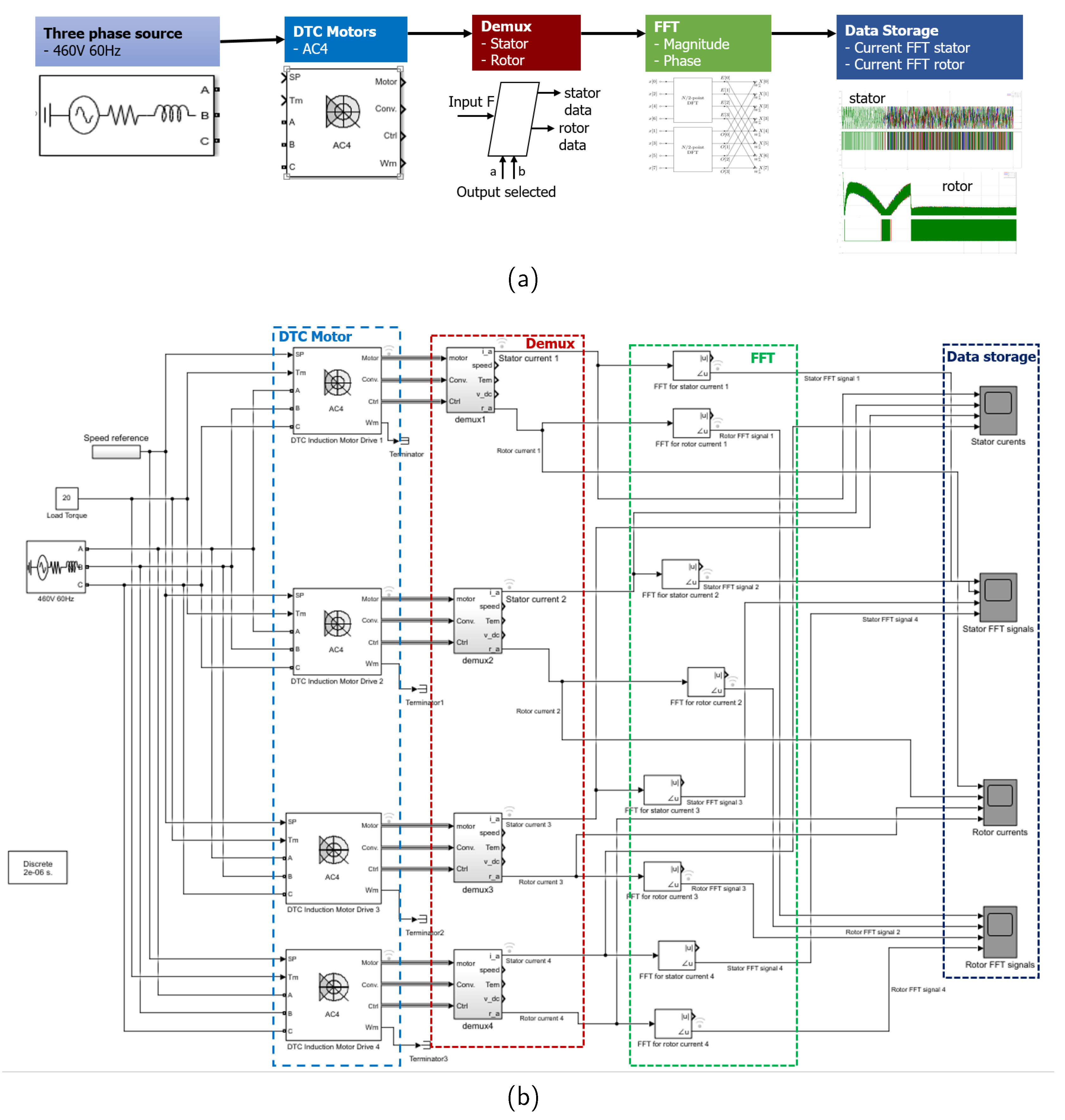Figure 1 illustrates the modeling and data acquisition approach, which consists of a general concept depicted in Figure 1a, and a more detailed representation involving four DTC motors shown in Figure 1b.

In the context of DTC, Demultiplexing (DEMUX) can be employed to separate different operating parameters of the motor, such as speed, torque, and current, into distinct output signals [33]. DTC is a technique used to manage the speed and torque of an induction motor by monitoring the currents flowing through the stator and making appropriate adjustments to the inverter’s switching patterns. Accurate and ongoing measurement of the stator currents and rotor position is crucial for the proper operation of DTC. Using DEMUX, the stator current and rotor position signals can be separated into independent output signals, enabling more precise control of the motor’s torque and speed [34].

3.1.1. DEMUX for DTC Motor

The AC4 motor drive also called the DTC Induction Motor Drive block, is a frequently utilized element within the Simscape Specialized Power Systems library. It is an enhanced control drive tailored for induction motors, offering direct torque and flux control functionalities. This drive incorporates closed-loop speed control and utilizes hysteresis-band torque and flux controllers.

Utilizing DEMUX in DTC offers multiple benefits. Firstly, it improves the performance of the motor by isolating different operating parameters, such as speed, torque, and current, and subsequently adjusting the control strategy based on these parameters. This enhances the efficiency and accuracy of the control system [35]. Moreover, demultiplexing the stator current and rotor position signals improves the accuracy of these measurements, thereby enhancing the overall performance of the DTC control system. It is crucial to emphasize the importance of accurately measuring the stator currents and rotor position for the proper functioning of DTC control. By incorporating demultiplexing techniques to separate the stator current and rotor position signals, the accuracy of these measurements can be improved, leading to enhanced performance of the DTC control system.

The DEMUX operation in DTC involves separating the stator current into its direct-axis and quadrature-axis components. This separation allows for independent control of these components, which is necessary for accurate torque and flux control. The DEMUX operation can be represented mathematically as:

r s c_s d = i_{s} \times c o s (θ_{r})

(1)

r s c_s q = i_{s} \times s i n (θ_{r})

(2)

where

i_{s}

represents the stator current vector,

θ_{r}

denotes the rotor position, and

r s c_s d

and

r s c_s q

represent the direct-axis and quadrature-axis of the stator current components, respectively.

The rotor current vector represents the current flowing through the rotor windings and is essential for accurate motor control. The rotor current vector, denoted as

r r c_r d q

, can be obtained using the following equations:

r r c_r d = r s c_s d \times c o s (θ_{r}) - r s c_s q \times s i n (θ_{r})

(3)

r r c_r q = r s c_s d \times s i n (θ_{r}) + r s c_s q \times c o s (θ_{r})

(4)

where

r r c_r d

represents the direct-axis component of the rotor current, and

r r c_r q

represents the quadrature-axis component of the rotor current.

3.1.2. FFT-Based Signal Processing

FFT is a mathematical technique that can be used to analyze the frequency components of a signal. The output signals of the DEMUX component for each induction motor can be used via FFT to extract relevant information about the frequency characteristics of the stator currents and rotor position data. By using FFT for the stator currents and rotor position signals, we can derive the frequency spectrum of the signals. It can assist in determining the dynamics of the motor and identify any unusual circumstances, such as stator winding flaws, rotor flaws, or other types of failures.

We can use mathematical equations and programming tools to calculate the FFT of the stator current and rotor current signals obtained from the DEMUX output of an induction motor. Here is a general procedure to calculate the FFT using mathematical equations:

Prepare the input data: the stator current vector as $r s c [n]$ and the rotor current vector as $r r c [n]$ , where n represents the discrete time index.

$S [k] = \sum_{k = 0}^{M - 1} (r s c [n] \times e x p (\frac{- i \times 2 \times π \times k \times n}{M}))$

(5)

$R [k] = \sum_{k = 0}^{M - 1} (r r c [n] \times e x p (\frac{- i \times 2 \times π \times k \times n}{M}))$

(6)

where $S [k]$ and $R [k]$ are the complex-valued spectrum of the stator current and rotor current signals, respectively. $r s c [n]$ and $r r c [n]$ are the stator current and rotor current signals at discrete time index n. M is the length of the stator current and rotor current vectors.
Extract the magnitude and phase information: To obtain the magnitude and phase information from the complex-valued FFT results, we can calculate the absolute value (magnitude) and phase angle of each FFT bin.

$M a g_S [k] = a b s (S [k])$

(7)

$M a g_R [k] = a b s (R [k])$

(8)

$P h a_S [k] = a t a n 2 (I m (S [k]), R e (S [k]))$

(9)

$P h a_R [k] = a t a n 2 (I m (R [k]), R e (R [k]))$

(10)

where $M a g_S [k]$ and $M a g_R [k]$ are the magnitudes of the complex-valued FFT results for the stator current and rotor current signals, respectively. $P h a_S [k]$ and $P h a_R [k]$ are the phase angles of the complex-valued FFT results for the stator current and rotor current signals, respectively. $I m (S [k])$ and $R e (R [k])$ represent the imaginary and real parts of $S [k]$ , respectively. $I m (R [k])$ and $R e (R [k])$ represent the imaginary and real parts of $R [k]$ , respectively.

3.2. Bi-LSTM Model Architecture

In this section, we provide detail of our Bi-LSTM model approach. Figure 2 illustrates the general architecture of the proposed method, while the proposed model training and forecasting evaluation is pointed out in Algorithm 1.

During preprocessing, we employ the MinMaxScaler function from the scikit-learn library to preprocess the data. This step is crucial as normalizing the data has been shown to enhance the performance of neural networks. The data transformation process involves three key steps. Firstly, we fit the scaler using the available training data, which entails estimating the minimum and maximum observable values based on the training data. Subsequently, we apply the scaler to the training data. Finally, we apply the same scaler to the test data. The MinMaxScaler technique is widely utilized for normalizing data, enabling the scaling of dataset values to a predefined range, often between 0 and 1. The mathematical formulation of the MinMaxScaler for FFT-transformed current data is as follows:

S_{i}_s c a l e d = \frac{S_{i} - S_m i n}{S_m a x - S_m i n}

(11)

where

S_{i}

S_m i n

S_m a x

are an individual sample, the minimum value, the maximum value from the FFT stator current data S,

S_{i}_s c a l e d

is the scaled value of

S_{i}

in the range

[0, 1]

R_{i}_s c a l e d = \frac{R_{i} - R_m i n}{R_m a x - R_m i n}

(12)

where

R_{i}

R_m i n

R_m a x

are an individual sample, the minimum value, the maximum value from the FFT rotor current data R,

R_{i}_s c a l e d

is the scaled value of

R_{i}

in the range

[0, 1]

Algorithm 1 Model Training and Forecasting Evaluation

Require:: $f s c$ , $f r c$
Ensure:: Forecasting unseen FFT stator current $s e g_f s c$ ,

Forecasting unseen FFT rotor current $s e g_f r c$
1:: Data preprocessing using $M i n M a x S c a l e$ method:

$r, s \leftarrow M i n M a x S c a l e (f s c, f r c)$
2:: Split preprocessed data into training and testing data with a ratio of 80:20, respectively

// For rotor data:

$r_t r, s_t r \leftarrow r [: l e n (r) \times 0.8], r [l e n (r) \times 0.8 :]$

// For stator data:

$r_t e, s_t e \leftarrow s [: l e n (s) \times 0.8], s [l e n (s) \times 0.8 :]$
3:: Create function $s p l i t_I O ()$ to split input and output from training and testing data

$(X r_t r, y r_t r), (X r_t e, y r_t e) \leftarrow s p l i t_I O (r_t r, r_t e)$

$(X s_t r, y s_t r), (X s_t e, y s_t e) \leftarrow s p l i t_I O (s_t r, s_t e)$
4:: Setup several hyperparameters of Bi-LSTM model:

$n_{i}, n_{h}, n_{o} \leftarrow n u m b e r o f i n p u t, h i d d e n, o u t p u t n o d e s$

$o p \leftarrow t r a i n i n g o p t i m i z e r$

$l o s s \leftarrow t r a i n i n g l o s s f u n c t i o n$

$v a l \leftarrow v a l i d a t i n g s p l i t v a l u e$

$c a l l \leftarrow E a r l y S t o p p i n g f u n c t i o n$
5:: while $i \leq e p o c h s (e p)$ do
6:: Create BiLSTM layer:

$B i L S T M \leftarrow L S T M (n_{i}, n_{h}, n_{o}, n_{f}, o p, l o s s)$
7::    Create $f i t ()$ function to learn:

    $f_r \leftarrow B i L S T M . f i t (X r_t r, y r_t r, e p, v a l, b a t, c a l l)$

    $f_s \leftarrow B i L S T M . f i t (X s_t r, y s_t r, e p, v a l, b a t, c a l l)$
8:: end while
9:: Training evaluation

$m s e_r, m s e_s \leftarrow f_r [l o s s], f_s [l o s s]$
10:: Testing evaluation

$s e g_f r c \leftarrow B i L S T M . p r e d i c t i o n (X r_t e)$

$s e g_f s c \leftarrow B i L S T M . p r e d i c t i o n (X s_t e)$
11:: Calculate RMSE and MAE losses

$e r r o r_r \leftarrow s e g_f r c - y r_t e$

$e r r o r_s \leftarrow s e g_f s c - y s_t e$

$r m s e_r \leftarrow s q r t (m e a n ((s q u a r e (e r r o r_r))))$

$r m s e_s \leftarrow s q r t (m e a n ((s q u a r e (e r r o r_s))))$

$m a e_r \leftarrow m e a n (a b s (e r r o r_r))$

$m a e_s \leftarrow m e a n (a b s (e r r o r_s))$
12:: return $s e g_f r c, s e g_f s c$

The Bi-LSTM architecture is an RNN type that excels at capturing long-term dependencies in sequential data. In contrast to traditional RNNs, which process data in a single direction, Bi-LSTMs simultaneously process input data in both forward and backward directions. This bidirectional processing enables the network to gather information from past and future contexts effectively. Our proposed Bi-LSTM model comprises multiple layers of Bi-LSTM units, each followed by a dense layer with a linear activation function. The input to the model is a sequence of historical electrical signal data, and the output is the predicted value for the next time step. To train the Bi-LSTM model, we employ the backpropagation algorithm with the Mean Squared Error (MSE) loss function. For optimization, we utilize the Adam optimizer, a widely-used algorithm for training Deep Neural Networks (DNNs). The outputs from both directions of the Bi-LSTM are combined through concatenation and passed through a fully connected layer, followed by an activation function, to generate the final output.

The forward LSTM can be represented as:

h_{t}^{f} = σ_{f} (W_{f} x_{t} + U_{f} h_{t - 1}^{f} + b_{f})

(13)

\begin{matrix} c_{t}^{f} = f_{f} (W_{f} x_{t} + U_{f} h_{t - 1}^{f} + b_{f}) ⊙ c_{t - 1}^{f} + i_{f} (W_{f} x_{t} + U_{f} h_{t - 1}^{f} + b_{f}) ⊙ tanh (W_{f} x_{t} + U_{f} h_{t - 1}^{f} + b_{f}) \end{matrix}

(14)

where

x_{t}

is the input at time step t (we assume that

x_{t}

represents for FFT stator current S or FFT rotor current R),

h_{t}^{f}

is the hidden state of the forward LSTM at time step t,

c_{t}^{f}

is the cell state of the forward LSTM at time step t,

W_{f}

U_{f}

, and

b_{f}

are the weights and biases of the forward LSTM,

σ_{f}

is the sigmoid activation function,

f_{f}

is the forget gate,

i_{f}

is the input gate, and ⊙ denotes element-wise multiplication.

The backward LSTM can be represented as:

h_{t}^{b} = σ_{b} (W_{b} x_{t} + U_{b} h_{t + 1}^{b} + b_{b})

(15)

\begin{matrix} c_{t}^{b} = f_{b} (W_{b} x_{t} + U_{b} h_{t + 1}^{b} + b_{b}) ⊙ c_{t + 1}^{b} + i_{b} (W_{b} x_{t} + U_{b} h_{t + 1}^{b} + b_{b}) ⊙ tanh (W_{b} x_{t} + U_{b} h_{t + 1}^{b} + b_{b}) \end{matrix}

(16)

where

h_{t}^{b}

and

c_{t}^{b}

are the hidden state and cell state of the backward LSTM at time step t, respectively,

W_{b}

U_{b}

, and

b_{b}

are the weights and biases of the backward LSTM,

σ_{b}

is the sigmoid activation function,

f_{b}

is the forget gate,

i_{b}

is the input gate, and ⊙ denotes element-wise multiplication.

The output of the Bi-LSTM model can be computed as follows:

y_{t} = σ (W_{o} [h_{t}^{f}; h_{t}^{b}] + b_{o})

(17)

where

[h_{t}^{f}; h_{t}^{b}]

is the concatenation of the forward and backward hidden states,

W_{o}

and

b_{o}

are the weights and biases of the output layer, and

σ

is the activation function.

3.3. Model Training and Evaluation Setting

We conducted experiments on a simulation dataset to evaluate the effectiveness of the proposed Bi-LSTM model for forecasting electrical signals of three-phase DTC induction motors in ship environments. The dataset comprises three-phase DTC induction motor electrical signal data collected from ship environments. The proposed Bi-LSTM model was trained and evaluated using the collected and preprocessed data. The dataset was divided randomly into a training set (80%) and a testing set (20%). We employed the Adam optimizer with a learning rate 0.001 to train the model. The training was conducted with a batch size of 64 and a maximum of 100 epochs. To identify the best combination, we conducted experiments with various hyperparameters, including the number of LSTM layers, the number of neurons per layer, and the dropout rate. The specific hyperparameters utilized in our proposed methods can be found in Table 1. The GRU and BiLSTM models accept a 3D input of shape (no_training_samples, no_timesteps, no_features).

In order to evaluate the effectiveness of our approached model, three widely used evaluation metrics, specifically MSE, RMSE, and MAE, are utilized. These evaluation metrics act as indicators of the model’s precision. MSE is particularly useful in identifying outlier predictions with significant errors, as it emphasizes these errors due to the squaring operation in its calculation (refer to (18)). Since the squaring operation ensures that MSE is always non-negative, it provides a means to evaluate the model’s performance without considering the direction of errors. RMSE, on the other hand, is a widely used metric that quantifies the difference between predicted and actual values (refer to (19)). While RMSE is sensitive to outliers, MAE is less affected by them and still provides valuable insights into prediction accuracy. MAE, which differs slightly in definition from MSE, involves taking the absolute difference between model predictions and ground truth and averaging these absolute differences across the entire dataset (refer to (20)). The three measures are defined as follows:

M S E = \frac{1}{n} \sum_{i = 1}^{n} {(y_{i}^{t} - y_{i}^{p})}^{2}

(18)

R M S E = \sqrt{\frac{\sum_{i = 1}^{n} y_{i}^{t} - y_{i}^{p}}{n}}

(19)

M A E = \frac{1}{n} \sum_{i = 1}^{n} | y_{i}^{t} - y_{i}^{p} |

(20)

where n denotes the total number of samples,

y^{t}

and

y^{p}

represents the actual and predicted motor signal data at the i th second time data, respectively.

Furthermore, to evaluate the performance of the proposed Bi-LSTM model, we trained and assessed a GRU model using the same dataset and evaluation criteria. The GRU model, an RNN version, was created expressly to overcome the vanishing gradient problem and improve the performance of ordinary RNNs. The GRU model includes the update and reset gates. The update gate controls how much of the prior hidden state should be kept and how much new input should be incorporated into the current hidden state. The reset gate, on the other hand, controls how much of the last hidden state should be ignored and how much fresh input should be absorbed into the current hidden state.

4. Results and Discussion

This section delves into a comprehensive discussion of our experimental findings. Initially, we examine the impact of employing FFT analysis on the extracted stator and rotor current data. Subsequently, we assess the performance of our proposed method by utilizing various loss metrics, including MSE, for both the training and validation processes and RMSE and MAE for the testing process, on the FFT stator current and FFT rotor current. Additionally, we validate the effectiveness of our proposed Bi-LSTM approach by contrasting its accuracy with that of the contemporary GRU time series forecasting model. Lastly, we present compelling evidence of the superior forecasting performance of our proposed method compared to the GRU model when applied to the same experimental data.

4.1. Effect of FFT Stator and Rotor Current Data

In this section, we delve into applying the FFT method for extracting valuable information from DTC induction motors’ stator and rotor current data. The FFT method is a widely used technique in signal processing that converts time-domain signals into the frequency domain. By leveraging this transformation, we can gain deeper insights into the spectral characteristics and frequency components present in the motor currents.

The effectiveness of employing the FFT method in different domains for signal analysis has been well-established. For example, the FFT technique has been utilized in power systems to examine power quality concerns like harmonic distortion and voltage fluctuations [36]. Similarly, in vibration analysis, the FFT method has been widely used to identify and analyze the frequency components of mechanical vibrations, aiding in detecting faults and anomalies in rotating machinery [37].

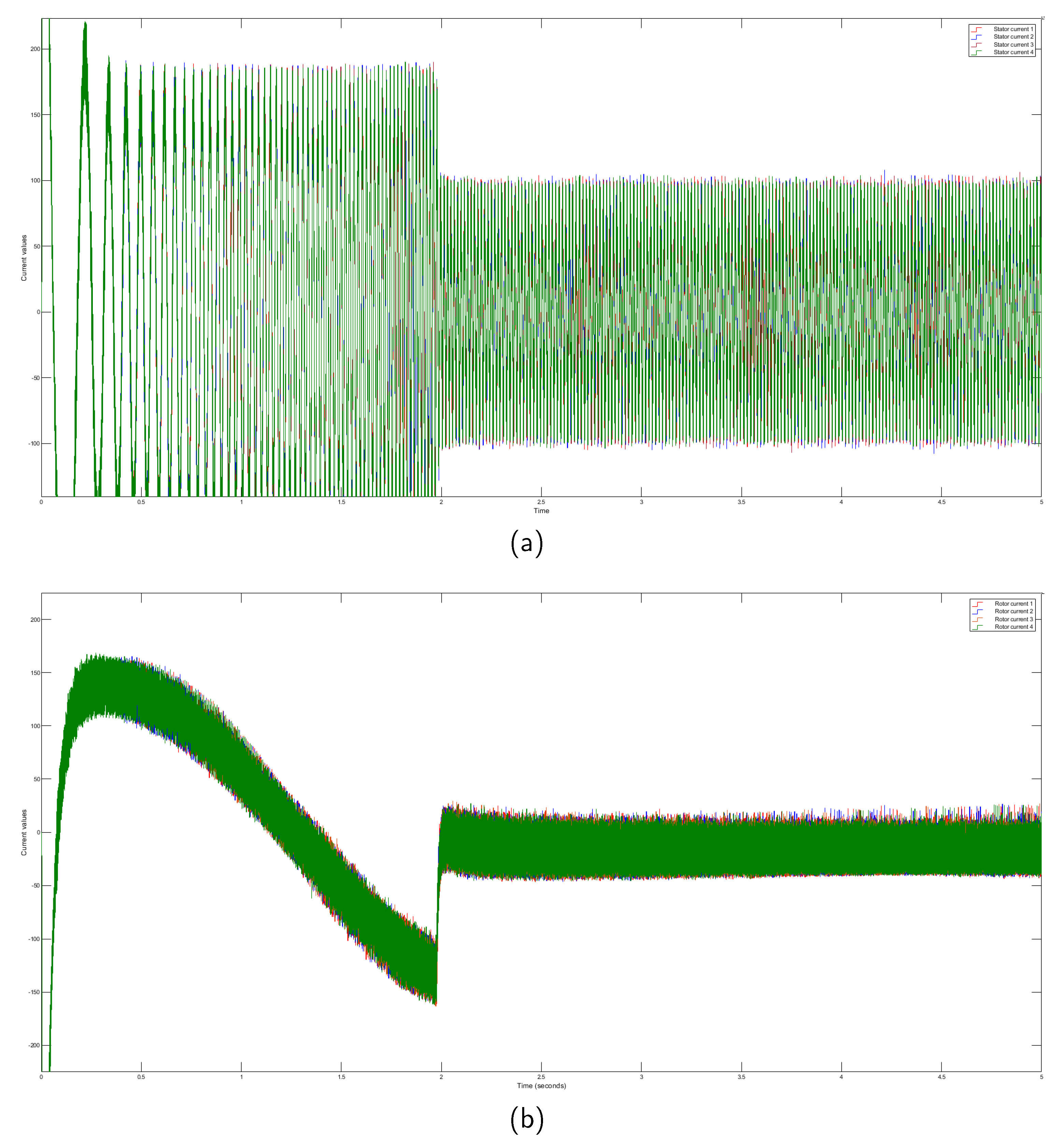
First, we analyze the raw data obtained from four identical DTC induction motors. We plot the stator and rotor current data on a single graph to provide a comprehensive overview, as Figure 3 demonstrates. However, the raw data exhibit inherent variability, presenting interpretation and further analysis challenges. Upon closer examination, we observe minor differences among the raw stator signals acquired from the four motors, as illustrated in Figure 3a. Similarly, we note slight disparities in the rotor signals, as depicted in Figure 3b. However, discerning or distinguishing these signals with the naked eye proves to be quite arduous. It poses substantial difficulties when identifying or forecasting patterns within these seemingly similar motor signal datasets.

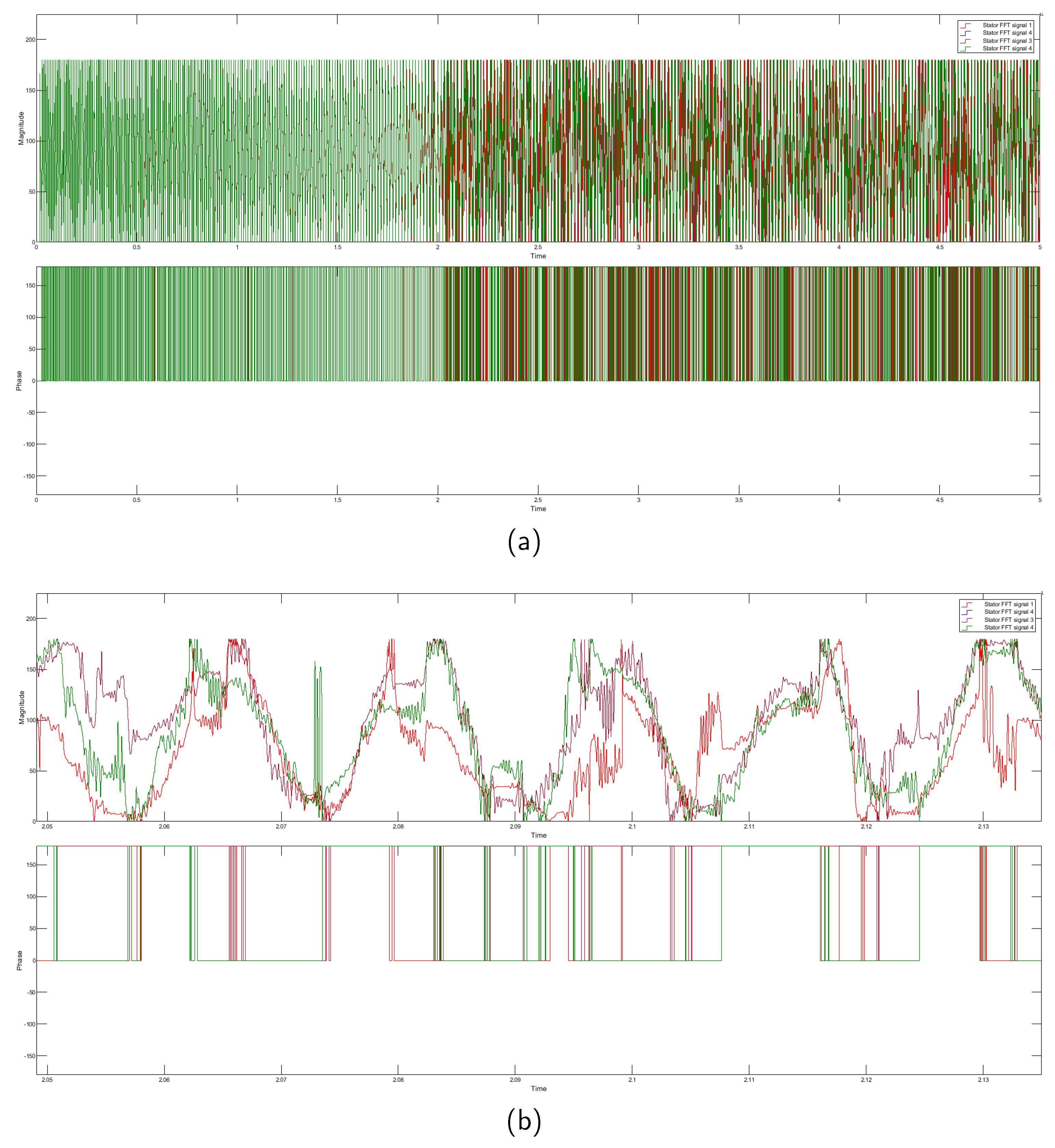
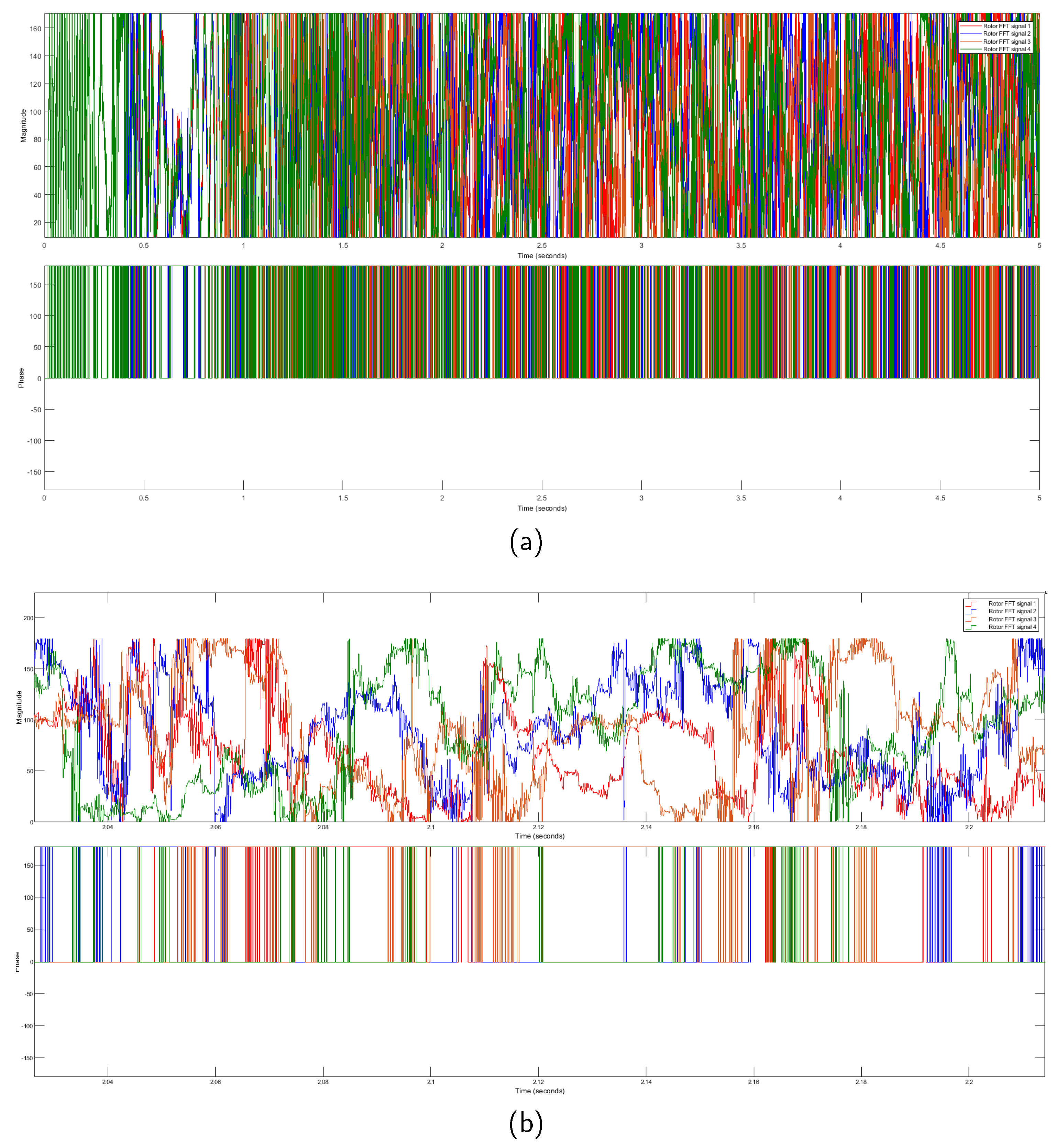
We employ the FFT extraction method to address the challenges posed by the variability in the raw data. This technique transforms the raw time-domain signals into frequency-domain signals, yielding magnitude and phase data. The resulting FFT stator and rotor signals are presented in Figure 4 and Figure 5, respectively. These frequency-domain signals exhibit distinct magnitudes and phases, providing valuable information for further analysis and processing, such as forecasting or classification tasks.

Comparing the raw data with the extracted frequency-domain data reveals significant differences among the same four motor signals. This disparity is clearly demonstrated in Figure 4 (FFT stator current data) and Figure 5 (FFT rotor current data). In order to provide a more detailed examination of the FFT stator and rotor current data, we zoom in on the plots, as illustrated in Figure 4b and Figure 5b, respectively.

The observed dissimilarities in the FFT representation of the four DTC induction motor signals highlight the effectiveness of the FFT method in capturing and distinguishing important features. Consequently, we utilize the FFT stator and rotor currents to evaluate our proposed approach.

4.2. Comparison Forecasting Performance of GRU and Bi-LSTM Models

Using simulation data, we assess our proposed Bi-LSTM model in forecasting electrical signals of three-phase DTC induction motors in ship environments. Our evaluation includes analyzing the impact of utilizing FFT on the stator and rotor current data through various performance metrics, such as MSE loss for training and validation and RMSE and MAE losses for testing. Additionally, we compare the performance of our proposed method, which utilizes a Bi-LSTM model for time-series forecasting, with that of the modern GRU time-series forecasting model.

4.2.1. Loss Metrics Measurement

To evaluate the effectiveness of the suggested approach, the Mean Squared Error (MSE) loss was calculated for both the training and validation sets, as presented in Table 2. In both the training and validation processes, the Bi-LSTM model demonstrated superior performance compared to the GRU model for both stator and rotor data. Moreover, our results indicated that the proposed model achieved slightly higher accuracy in predicting the motor’s FFT stator currents than the FFT rotor currents.

We conducted additional evaluations of the proposed Bi-LSTM model by measuring MAE and RMSE on the testing data, and the results are presented in Table 3. The findings demonstrate that the proposed model surpassed the standard GRU model regarding accuracy and prediction error. Specifically, we compared the predicted stator current of the Bi-LSTM and GRU models to the actual stator current and calculated the MSE and RMSE values. The lower MSE and RMSE values indicate that the proposed model can accurately predict the FFT rotor current.

4.2.2. Forecasting Evaluation Illustration

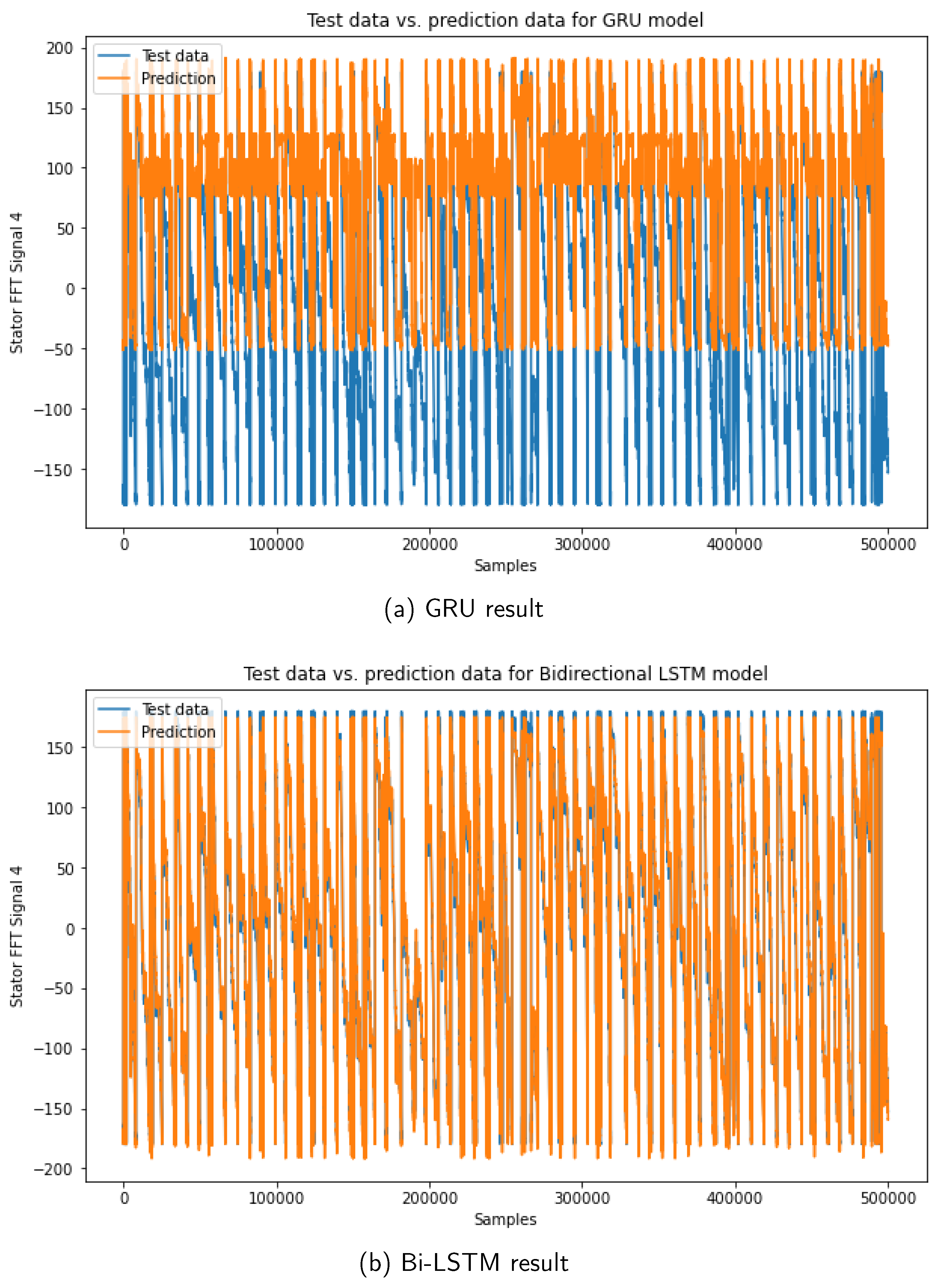
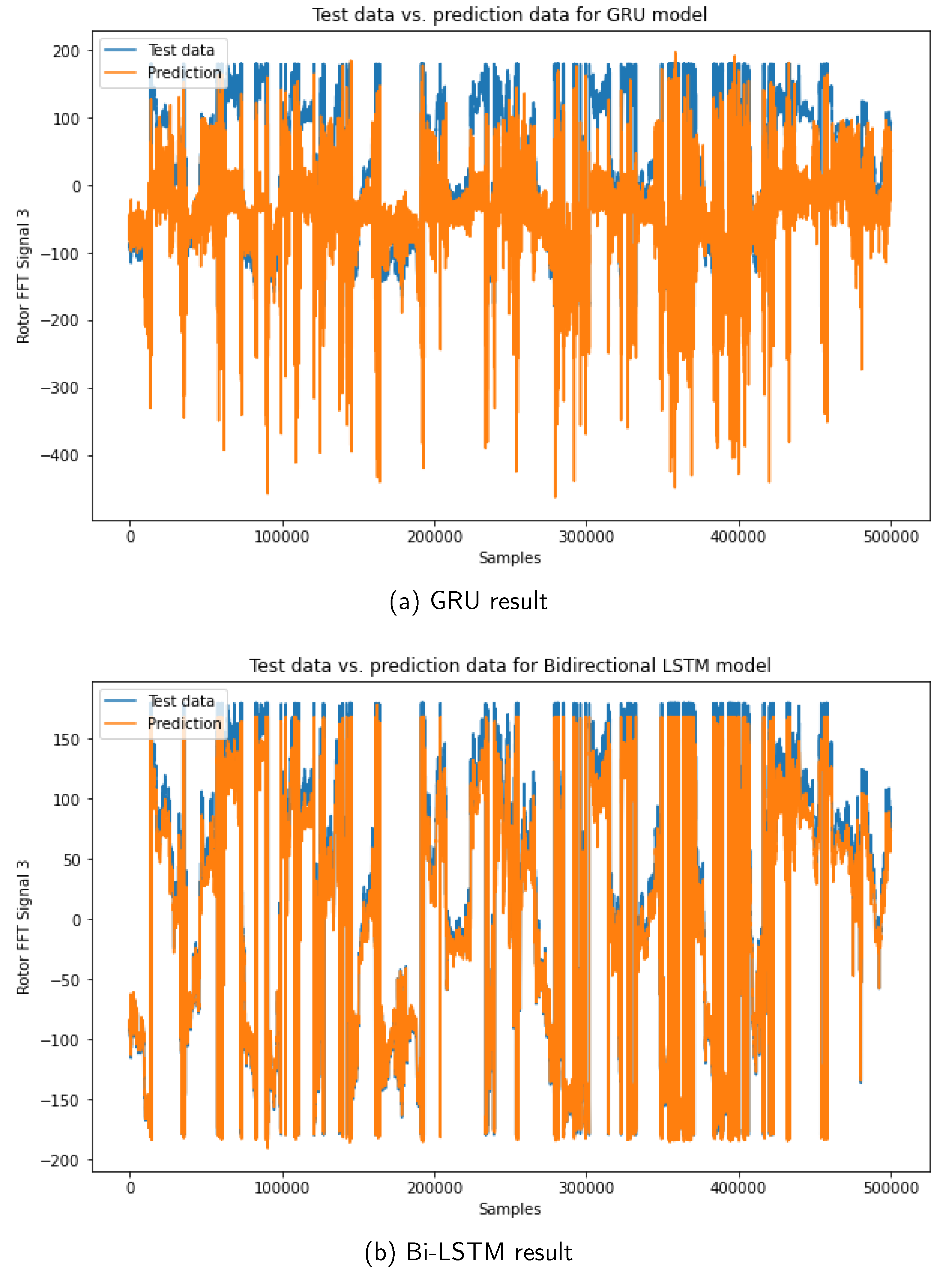
The forecasting evaluation results of the Bi-LSTM and GRU models on both datasets are presented in Figure 6 and Figure 7. In particular, Figure 6 illustrates the FFT stator forecasting results of motor 4, clearly showcasing the superior performance of the Bi-LSTM model compared to the GRU model. The predicted stator current signals generated by the Bi-LSTM model exhibit a closer alignment with the actual signals, indicating better accuracy and precision than the GRU model. Likewise, Figure 7 demonstrates the notable superiority of the Bi-LSTM model in predicting FFT rotor data. The predicted rotor current signals produced by the Bi-LSTM model exhibit reduced noise and improved accuracy compared to the GRU model. These compelling findings underscore the outstanding performance of the Bi-LSTM model in accurately forecasting the electrical signals of three-phase DTC induction motors in ship environments.

In summary, the comparative evaluation against conventional GRU models underscores the exceptional performance of the proposed Bi-LSTM model. It exhibits superior accuracy and lower prediction error when considering stator and rotor data. The evaluation metrics, including MSE, RMSE, and MAE, reveal that the model achieves low error values, indicating its effectiveness in accurately forecasting the FFT stator and rotor currents. The Bi-LSTM model exhibits higher accuracy in predicting the FFT stator current of the motor, further emphasizing its proficiency in capturing complex patterns and trends in the data.

5. Conclusion

This paper presented a novel approach for forecasting electrical signals in three-phase DTC induction motors operating in ship environments. Accurate prediction of these signals is crucial for achieving optimal motor performance and enabling effective condition monitoring. By leveraging the transformed FFT and Bi-LSTM network, we were able to capture the complex dynamics of multiple induction motors and evaluate the performance of our proposed Bi-LSTM model. Our results demonstrated that our approach achieved high accuracy in forecasting electrical signals, surpassing the performance of the GRU model. It highlights the effectiveness of the Bi-LSTM model in capturing the temporal dependencies present in the data. The findings of this study provide valuable insights into the development of accurate forecasting models for DTC induction motors, which can lead to enhanced motor performance, improved condition monitoring, and increased operational efficiency. Future research can further enhance the methodology and investigate its applicability in other motor control systems.

Author Contributions

Conceptualization, T.T.H.L. ; methodology, T.T.H.L. and Y.E.O; software, T.T.H.L. and U.J.; validation, T.T.H.L., Y.E.O, and H.K.; formal analysis, T.T.H.L. and Y.E.O; investigation, Y.E.O and U.J.; resources, T.T.H.L.; data curation, T.T.H.L. and Y.E.O ; writing—original draft preparation, T.T.H.L. and Y.E.O; writing—review and editing, T.T.H.L. and H.K.; visualization, T.T.H.L. and U.J.; supervision, T.T.H.L. and H.K.; project administration, H.K.; funding acquisition, H.K. All authors have read and agreed to the published version of the manuscript.

Funding

This research was supported by the MSIT(Ministry of Science and ICT), Korea, under the ITRC(Information Technology Research Center) support program(IITP-2023-2020-0-01797) supervised by the IITP(Institute for Information & Communications Technology Planning & Evaluation).

Informed Consent Statement

Not applicable.

Conflicts of Interest

The authors declare no conflict of interest.

Abbreviations

The following abbreviations are used in this manuscript:

DTC	Direct Torque Control
FFT	Fast Fourier Transform
Bi-LSTM	Bi-directional Long Short-Term Memory
GRU	Gated Recurrent Unit
ANNs	Artificial Neural Networks
DL	Deep Learning
RNN	Recurrent Neural Network
CNNs	Convolutional Neural Networks
MAE	Mean Absolute Error
DEMUX	Demultiplexing
MSE	Mean Squared Error
DNNs	Deep Neural Networks

References

Aktas, M.; Awaili, K.; Ehsani, M.; Arisoy, A. Direct torque control versus indirect field-oriented control of induction motors for electric vehicle applications. Engineering Science and Technology, an International Journal 2020, 23, 1134–1143. [Google Scholar] [CrossRef]
Diab, A. A. Z.; Elsawy, M. A.; Denis, K. A.; Alkhalaf, S.; Ali, M.Z. Artificial neural based speed and flux estimators for induction machine drives with matlab/simulink. Mathematics 3390, 10. [Google Scholar] [CrossRef]
Afrasiabi, S.; Afrasiabi, M.; Parang, B.; Mohammadi, M. Realtime bearing fault diagnosis of induction motors with accelerated deep learning approach. In Proceedings of the 2019 10th international power electronics, drive systems and technologies conference (PEDSTC), Shiraz, Iran, 12-14 February 2019. [Google Scholar]
Mohamed, H.; Abdelmadjid, B.; Lotfi, B. Performance improvement of svm-dtc of induction machine drive via backstepping controller and stator resistance compensator. In Proceedings of the 2019 International Conference on Advanced Electrical Engineering (ICAEE), Algiers, Algeria, 19-21 November 2019. [Google Scholar]
Aher, K. S.; Thosar, A. Modeling and simulation of five phase induction motor using matlab/simulink. Int. J. Eng. Res. Appl 2016, 5, 1–8. [Google Scholar]
Premkumar, K.; Manikandan, B. V. Adaptive Neuro-Fuzzy Inference System based speed controller for brushless DC motor. Neurocomputing 2014, 138, 260–270. [Google Scholar] [CrossRef]
Shi, K.; Chan, T.; Wong, Y.; Ho, S. L. Modelling and simulation of the three-phase induction motor using simulink. International journal of electrical engineering education 1999, 36, 163–172. [Google Scholar] [CrossRef]
Vukadinovic, D.; Basic, M.; Kulisic, L. Stator resistance identification based on neural and fuzzy logic principles in an induction motor drive. Neurocomputing 2010, 73, 602–612. [Google Scholar] [CrossRef]
Makinde, K. A.; Bakare, M. S.; Akinloye, B. O.; Amole, A. O.; Adewuyi, O. B.; Zubair, U. O.; Owonikoko, W. O. Simulation based testing and performance investigation of induction motor drives using matlab simulink. SN Applied Sciences 2023, 5, 73. [Google Scholar] [CrossRef]
Lascu, C.; Boldea, I.; Blaabjerg, F. Direct torque control of sensorless induction motor drives: a sliding-mode approach. IEEE Transactions on Industry Applications 2004, 40, 582–590. [Google Scholar] [CrossRef]
Zhang, J.; Kang, L.; Chen, L.; Yi, B.; Xu, Z. Direct torque control of sensorless induction machine drives: a two-stage kalman filter approach. Mathematical Problems in Engineering 2015, 2015. [Google Scholar] [CrossRef]
Ghods, A.; Lee, H. H. Probabilistic frequency-domain discrete wavelet transform for better detection of bearing faults in induction motors. Neurocomputing 2016, 188, 206–216. [Google Scholar] [CrossRef]
Le, T.-T.-H.; Heo, S.; Kim, H. Toward load identification based on the hilbert transform and sequence to sequence long shortterm memory. IEEE Transactions on Smart Grid 2021, 12, 3252–3264. [Google Scholar] [CrossRef]
Aldhyani, T.H.H.; Alkahtani, H. A Bidirectional Long Short-Term Memory Model Algorithm for Predicting COVID-19 in Gulf Countries. Life 2021, 11, 1118. [Google Scholar] [CrossRef]
Noor, F.; Haq, S.; Rakib, M.; Ahmed, T.; Jamal, Z.; Siam, Z.S.; Hasan, R.T.; Adnan, M.S.G.; Dewan, A.; Rahman, R.M. Water Level Forecasting Using Spatiotemporal Attention-Based Long Short-Term Memory Network. Water 2022, 14, 612. [Google Scholar] [CrossRef]
Alharbi, F.R.; Csala, D. Wind Speed and Solar Irradiance Prediction Using a Bidirectional Long Short-Term Memory Model Based on Neural Networks. Energies 2021, 14, 6501. [Google Scholar] [CrossRef]
Wang, Y.; Feng, B.; Hua, Q.-S.; Sun, L. Short-Term Solar Power Forecasting: A Combined Long Short-Term Memory and Gaussian Process Regression Method. Sustainability 2021, 13, 3665. [Google Scholar] [CrossRef]
Le-Huy, H. Modeling and simulation of electrical drives using matlab/simulink and power system blockset. In Proceedings of the IECON’01. 27th Annual Conference of the IEEE Industrial Electronics Society (Cat. No.37243); 2001; Volume 3, pp. 1603–1611. [Google Scholar] [CrossRef]
Bozin, A. Electrical power systems modeling and simulation using simulink. In Proceedings of the IEE Colloquium on The Use of Systems Analysis and Modelling Tools: Experiences and Applications (Ref. No. 1998/413); 1998; pp. 10/1–10/8. [Google Scholar] [CrossRef]
Beliczynski, B.; Grzesiak, L. Induction motor speed estimation: neural versus phenomenological model approach. Neurocomputing 2002, 43, 17–36. [Google Scholar] [CrossRef]
Xia, Y.; Oghanna, W. Study on fuzzy control of induction machine with direct torque control approach. In Proceedings of the ISIE ’97 Proceeding of the IEEE International Symposium on Industrial Electronics, Guimaraes, Portugal, 7-11 July 1997; Volume 2, pp. 625–630. [Google Scholar] [CrossRef]
Buja, G.; Kazmierkowski, M. Direct torque control of pwm inverterfed ac motors - a survey. IEEE Transactions on Industrial Electronics 2004, 514, 744–757. [Google Scholar] [CrossRef]
Grabowski, P.; Kazmierkowski, M.; Bose, B.; Blaabjerg, F. A simple direct-torque neuro-fuzzy control of pwm-inverter-fed induction motor drive. IEEE Transactions on Industrial Electronics 2000, 47, 863–870. [Google Scholar] [CrossRef]
Lai, Y.-S.; Chen, J.-H. A new approach to direct torque control of induction motor drives for constant inverter switching frequency and torque ripple reduction. IEEE Transactions on Energy Conversion 2001, 16, 220–227. [Google Scholar] [CrossRef]
Jalali, S. M. J.; Ahmadian, S.; Khosravi, A.; Shafie-khah, M.; Nahavandi, S.; CatalA£o, J. P. S. A novel evolutionary-based deep convolutional neural network model for intelligent load forecasting. IEEE Transactions on Industrial Informatics 2021, 17, 8243–8253. [Google Scholar] [CrossRef]
Amarasinghe, K.; Marino, D. L.; Manic, M. Deep neural networks for energy load forecasting. In Proceedings of the 2017 IEEE 26th International Symposium on Industrial Electronics (ISIE), Edinburgh, UK, 19-21 June 2017; pp. 1483–1488. [Google Scholar] [CrossRef]
Song, T.; Liu, C.; Wu, R.; Jin, Y.; Jiang, D. A hierarchical scheme for remaining useful life prediction with long short-term memory networks. Neurocomputing 2022, 487, 22–33. [Google Scholar] [CrossRef]
Ali, M. Z.; Shabbir, M. N. S. K.; Zaman, S. M. K.; Liang, X. Single-and multi-fault diagnosis using machine learning for variable frequency drive-fed induction motors. IEEE Transactions on Industry Applications 2020, 56, 2324–2337. [Google Scholar] [CrossRef]
Le, T.-T.-H.; Kang, H.; Kim, H. Household Appliance Classification Using Lower Odd-Numbered Harmonics and the Bagging Decision Tree. IEEE Access 2020, 8, 55937–55952. [Google Scholar] [CrossRef]
Nishat Toma, R.; Kim, J.-M. Bearing fault classification of induction motors using discrete wavelet transform and ensemble machine learning algorithms. Applied Sciences 2020, 10. Available online: https: //www.mdpi.com/2076-3417/10/15/5251. [CrossRef]
Koh, D.-Y.; Jeon, S.-J.; Han, S.-Y. Performance prediction of induction motor due to rotor slot shape change using convolution neural network. Energies 2022, 15. Available online: https://www.mdpi.com/1996-1073/15/11/4129. [CrossRef]
Hussein, A. S.; Hawas, M. N. Power quality analysis based on simulation and matlab/simulink. Indonesian Journal of Electrical Engineering and Computer Science 2019, 16, 1144–1153. [Google Scholar] [CrossRef]
Bansal, M.; Singh, H.; Sharma, G. A taxonomical review of multiplexer designs for electronic circuits & devices. Journal of Electronics 2021, 3, 77–88. [Google Scholar]
Kim, Y. S. Analysis of starting torque and speed characteristics for squirrel cage induction motor according to material properties of rotor slot. Transactions on electrical and electronic materials 2015, 16, 328–333. [Google Scholar] [CrossRef]
Zhang, L.; Zhu, X.; Cui, R.; Han, S. A generalized open-circuit fault-tolerant control strategy for foc and dtc of five-phase fault-tolerant permanent-magnet motor. IEEE Transactions on Industrial Electronics 2021, 69, 7825–7836. [Google Scholar] [CrossRef]
Wang, S.; Chen, H. A novel deep learning method for the classification of power quality disturbances using deep convolutional neural network. Applied Energy 2019, 235, 1126–1140. Available online: https://www.sciencedirect.com/science/article/pii/ S0306261918314703. [CrossRef]
Gu, J.; Peng, Y.; Lu, H.; Chang, X.; Chen, G. A novel fault diagnosis method of rotating machinery via vmd, cwt and improved cnn. Measurement 2022, 200, 111635. Available online: https://www.sciencedirect.com/science/article/pii/ S0263224122008454. [CrossRef]

Figure 1. The modeling and data acquisition approach. (a) General concept of modeling and data acquisition; (b) Detailed depiction involving four DTC motors.

Figure 2. The architecture of the proposed method with unrolled structure of Bi-LSTM model.

Figure 3. Current stator and rotor signals from raw data. (a) Current stator signals. (b) Current rotor signals.

Figure 4. FFT signals of stator. (a) Magnitude and phase of stator FFT signals. (b) Magnified view of the magnitude and phase of stator FFT signals.

Figure 5. FFT signals of rotor. (a) Magnitude and phase of the rotor’s FFT signals. (b) Enlarged view of the magnitude and phase of the rotor’s FFT signals.

Figure 6. Comparison of stator FFT signal forecasting results between GRU and Bi-LSTM models: (a) Predicted stator FFT signal of motor 4 by the GRU model, and (b) Predicted stator FFT signal of motor 4 by the Bi-LSTM model.

Figure 7. Comparison of rotor FFT signal forecasting results between GRU and Bi-LSTM models: (a) Predicted FFT signal of motor 3 by the GRU model, (b) Predicted FFT signal of motor 3 by the Bi-LSTM model.

Table 1. Hyperparamters setting for GRU and Bi-LSTM models

Hyperparameters	Variable	Value
Number of training samples	no_training_samples	1,999,970
Number of testing samples	no_testing_sample	499,970
Number of time steps	no_timesteps	30
Number of input neurons	no_input_node ( $n i$ )	64
Number of hidden neurons	no_hidden_node ( $n h$ )	64
Number of output neurons	no_output_node ( $n o$ )	1
Number of features	no_features	1
Dropout layer	dropout	0.2
Training optimizer	optimizer ( $o p$ )	Adam
Batch size	batch_size ( $b a t$ )	16
Training shuffle	shuffle	false
Number of epochs	$e p o c h s$	100
Validation ratio	$v a l$	0.2

Table 2. MSE results of GRU and Bi-LSTM models for training and validating process

Evaluation	Model	Stator Data				Rotor Data
Process		Motor 1	Motor 2	Motor 3	Motor 4	Motor 1	Motor 2	Motor 3	Motor 4
Train	GRU	0.0012	0.0007	0.0008	0.0137	0.0011	0.0028	0.0045	0.0011
	Bi-LSTM	0.0003	0.0004	0.0006	0.0003	0.0006	0.0005	0.0006	0.0006
Validate	GRU	0.0006	0.0019	0.0005	0.0628	0.0019	0.00267	0.0465	0.0017
	Bi-LSTM	0.0005	0.0013	0.0012	0.0005	0.0006	0.0008	0.0015	0.0005

Table 3. MAE and RMSE results of GRU and Bi-LSTM models for testing process

Evaluation	Model	Stator Data				Rotor Data
Metric		Motor 1	Motor 2	Motor 3	Motor 4	Motor 1	Motor 2	Motor 3	Motor 4
MAE	GRU	88.8639	102.4355	92.3747	104.9523	90.4460	86.7933	83.8774	90.4395
	Bi-LSTM	86.3565	101.4268	87.1624	95.8002	81.8216	84.8299	46.1538	82.7156
RMSE	GRU	102.7566	114.9634	105.7504	105.8054	102.7570	98.8687	96.3640	102.6000
	Bi-LSTM	99.9575	114.9324	100.4124	104.9523	93.3045	95.1969	60.1075	94.5194

Disclaimer/Publisher’s Note: The statements, opinions and data contained in all publications are solely those of the individual author(s) and contributor(s) and not of MDPI and/or the editor(s). MDPI and/or the editor(s) disclaim responsibility for any injury to people or property resulting from any ideas, methods, instructions or products referred to in the content.

© 2023 by the authors. Licensee MDPI, Basel, Switzerland. This article is an open access article distributed under the terms and conditions of the Creative Commons Attribution (CC BY) license (http://creativecommons.org/licenses/by/4.0/).

Copyright: This open access article is published under a Creative Commons CC BY 4.0 license, which permit the free download, distribution, and reuse, provided that the author and preprint are cited in any reuse.

MDPI Initiatives

Important Links

Choose an area of interest and we will send you notifications of new preprints at your preferred frequency.

Disclaimer

Time Series Electrical Motor Drives Forecasting based on Simulation Modeling and Bidirectional Long-Short Term Memory

Abstract

1. Introduction

2. Related Work

3. Methodology

3.1. Modeling and Data Acquisition

3.1.1. DEMUX for DTC Motor

3.1.2. FFT-Based Signal Processing

3.2. Bi-LSTM Model Architecture

3.3. Model Training and Evaluation Setting

4. Results and Discussion

4.1. Effect of FFT Stator and Rotor Current Data

4.2. Comparison Forecasting Performance of GRU and Bi-LSTM Models

4.2.1. Loss Metrics Measurement

4.2.2. Forecasting Evaluation Illustration

5. Conclusion

Author Contributions

Funding

Informed Consent Statement

Conflicts of Interest

Abbreviations

References

MDPI Initiatives

Important Links

Subscribe