1. Introduction
Precise sales forecasts are of paramount importance to retailers as they heavily depend on them to effectively manage their supply chains and make crucial decisions related to marketing, logistics, finance, and human resources [
1]. Accurate sales forecasts help retailers determine how much inventory they need to purchase from their suppliers in order to meet customer demand [
2]. If the forecast is too low, they risk running out of stock and losing sales. If the forecast is too high, they risk overstocking and tying up cash in excess inventory. Sales forecasts also help retailers plan their logistics operations, such as determining how much warehouse space they need, how many trucks they need to transport goods, and how much labor is required to handle incoming and outgoing shipments. They also help retailers plan their marketing campaigns, such as determining which products to promote, which channels to use, and how much to spend on advertising [
3]. By having a clear understanding of expected sales volumes, retailers can allocate their marketing budgets more effectively. Accurate sales forecasts are also important for financial planning, such as budgeting and forecasting cash flow. Retailers need to know how much revenue they can expect in order to plan for expenses, investments, and debt repayment. Finally, sales forecasts are used by retailers to plan their staffing needs. They need to know how many employees they will need in their stores and warehouses in order to meet customer demand, and how much labor they will need to handle incoming and outgoing shipments [
4].
A global forecasting model, such as a Recurrent Neural Network (RNN), is a model that uses information from multiple time series to make predictions [
5,
6]. This is in contrast to a univariate forecasting model like ARIMA (Autoregressive Integrated Moving Average) or ETS (ExponenTial Smoothing) [
7,
8], which only use information from a single time series to make predictions. In a global forecasting model, the RNN is trained on multiple time series at once. Each time series is considered a separate input sequence, and the RNN is trained to capture the patterns and relationships between the different time series. This allows the model to make predictions for all of the time series simultaneously. One advantage of using a global forecasting model like a RNN is that it can capture complex dependencies and relationships between the different time series. For example, sales of one product in a store may be influenced by sales of a complementary product, or sales at one store may be influenced by sales at nearby stores. By using a global model that takes into account all of the relevant time series, we can better capture these relationships and make more accurate predictions [
9]. Another advantage of using a global model is that it can help reduce uncertainty in the individual time series. In some cases, individual time series may be noisy or exhibit erratic behavior. By using a global model that incorporates information from multiple time series, we can reduce the impact of these individual anomalies and improve the overall accuracy of the forecasts [
10].
In retail forecasting, covariates (also known as exogenous variables or features) can be used to help improve the accuracy of forecasts [
11]. Retail sales can be influenced by the time of year, as well as holidays, weekends, and other special events. Including calendar variables such as day of week, month, and year can help capture these effects. Changes in price can have a significant impact on sales too. Including variables such as regular price, discount percentage, and promotional price can help capture these effects. Promotions, advertising, and other marketing activities can also influence sales. Including variables such as the type and frequency of marketing activities can help capture these effects. Weather conditions can affect the demand for certain products. Including variables such as temperature, precipitation, and wind speed can help capture these effects. The characteristics of a store’s local area can also influence sales. Including variables such as population density, median income, and age distribution can help capture these effects. Overall economic conditions can also influence sales. Including variables such as unemployment rate, GDP, and consumer confidence can help capture these effects.
The objective of this research was to explore how the precision of global forecasting models is influenced by incorporating various potential demand covariates, considering their potential effects on operational decisions. The subsequent structure of this paper is organized as follows: In
Section 2, we outline the developed forecasting framework designed for the evaluation study, while
Section 3 delves into its implementation details. Moving forward,
Section 4 unveils and discusses the obtained results, and finally, in
Section 5, we offer concluding remarks along with identifying potential areas for further research.
2. Autoregressive neural network model
We utilize a sequence-to-sequence model called DeepAR [
12] to tackle the challenge of nonlinearity in time series data. DeepAR incorporates a recurrent neural network (RNN) to extend the traditional autoregressive model, allowing for more complex relationships in the data [
13,
14]. This model serves as a multivariate forecaster, generating probabilistic forecasts for future time series values based on their historical values (referred to as lags) and additional covariates [
15,
16].
In this context,
refers to the sales of product
i at time
t. The primary objective of the DeepAR model is to forecast the conditional probability
P of future sales
using past sales
and additional information in the form of covariates
, where
represents the first time instant of the future and
T represents the last time instant of the future [
17]:
It’s important to note that the time index t is relative, meaning that may not correspond to the initial time point of the time series. During training, we have access to in both the conditioning range and the prediction range . The former is used for encoding, while the latter is used for decoding in the sequence-to-sequence model. However, during inference (when we make predictions), is not available in the prediction range.
At each time step
t, the model produces an output represented by
:
This output is obtained by applying a multi-layer RNN with LSTM (long short-term memory) cells [
18], and it is parameterized by
. The model is considered autoregressive because it takes the sales value from the previous time step
as input. Additionally, it is is considered recurrent, as the output from the network at the previous time step
is given back as input at the next time step.
During training, we learn the model parameters by maximizing the log-likelihood of a chosen probability distribution using the equation:
Here, l denotes the likelihood of the distribution and represents a linear mapping from the function to the parameters of the distribution. DeepAR uses the entire time range to calculate the loss since the encoder model is identical to the decoder. DeepAR forecasts a single value at each step. However, during the inference phase, to predict several steps, the model obtains forecasts repeatedly for subsequent periods until the forecast horizon is reached. The model starts by generating samples from a probability distribution that has been trained on past sequences. The first prediction is made using these samples, and this prediction is then used as input to the model to make the next prediction. This process is repeated for each subsequent period. Because the predictions are derived from samples taken from the trained distribution, the model’s output is probabilistic. This means that the model does not produce a single deterministic value for each prediction, but rather a distribution of possible values. This distribution can be used to assess the forecasting accuracy of the model by providing a measure of the uncertainty associated with each prediction. The sampling mechanism also allows the model to be used to generate different forecasting scenarios. By sampling from the distribution of predictions, the model can be used to generate a range of possible outcomes, which can be used to inform decision-making.
Sales data often exhibits a zero-inflated distribution, meaning that there are a significant number of observations that equal zero [
19]. This can pose a challenge for forecasting models, as they are typically not designed to handle zeros. To address this challenge, we used the negative log-likelihood of the Tweedie distribution as our loss function [
20,
21]. The Tweedie distribution is a flexible distribution that can accommodate zero-inflated data, and the negative log-likelihood is a well-established loss function for Tweedie models. This approach allowed us to develop a forecasting model that was able to accurately predict both zero and non-zero sales.
Here, represents the gamma function, and and p denote the mean, dispersion, and power parameters, respectively. When p lies between 1 and 2, the distribution takes on the form of a compound Poisson-gamma distribution, which is frequently used for datasets displaying positive skewness and a significant number of zeros. The dispersion parameter regulates the level of diversity or heterogeneity in the data. A small value of suggests high dispersion in the data, whereas a large value indicates homogeneity.
3. Empirical study
3.1. Dataset
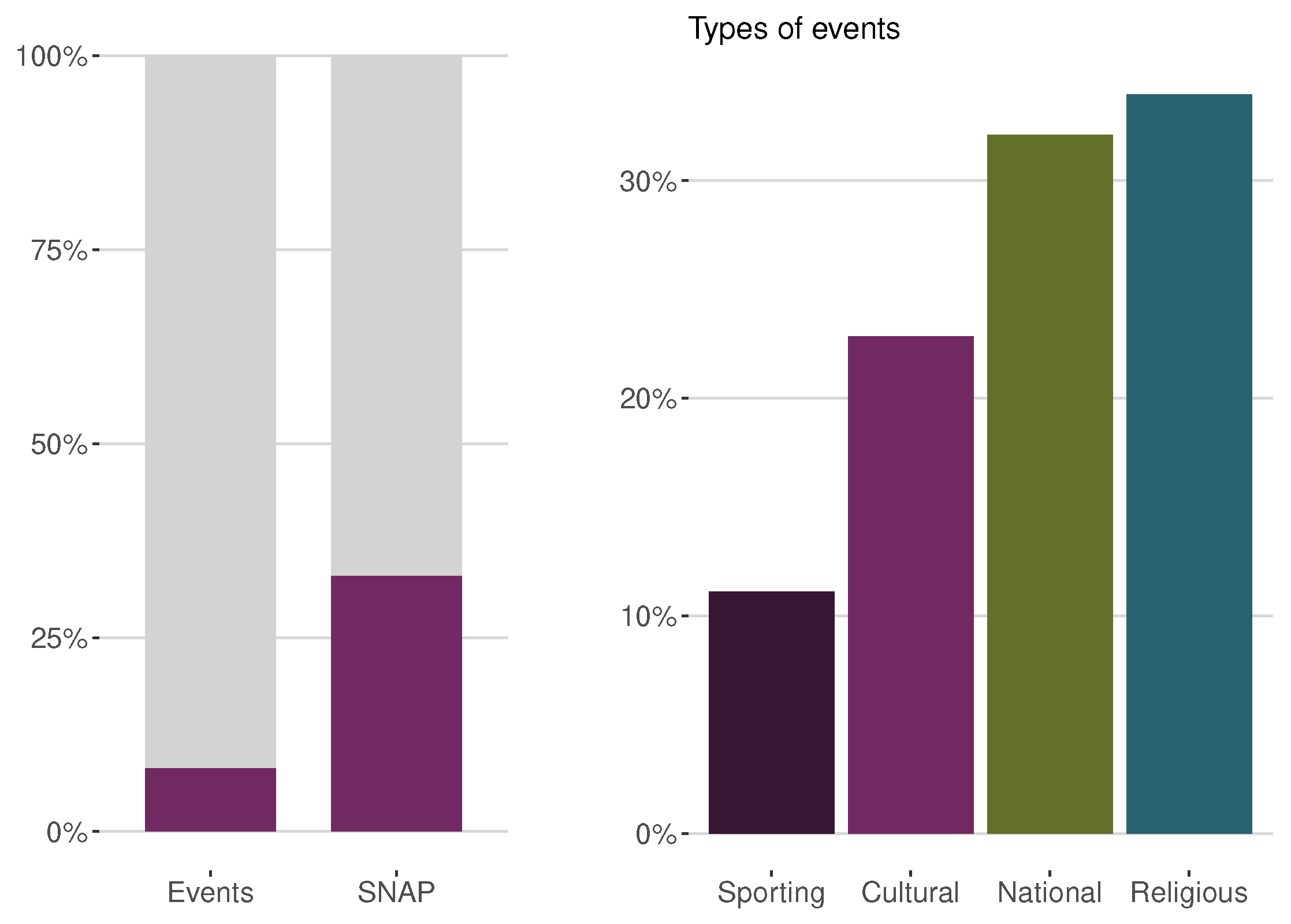
In this study, we used the M5 competition dataset, which is a well-established and openly available dataset of hierarchical unit sales data from Walmart. The M5 dataset is widely used for forecasting research because it is credible and reproducible. The M5 dataset includes 3,049 items from the Hobbies, Foods, and Household categories, which are disaggregated into seven departments. These items are sold on 10 stores located in three states: California, Texas, and Wisconsin. The dataset covers a period of 5.4 years, from January 29, 2011, to June 19, 2016, on a daily basis, totaling 1969 days. In addition to sales data, the M5 dataset also includes the regular price of each item, SNAP days, and special events that may impact sales. Approximately 8% of days in the dataset are marked by a special event, which is equivalent to around 160 events in the span of 1969 days. Of these events, around one-third are religious, such as Orthodox Christmas, while another one-third are national holidays, like Independence Day. The remaining third is divided into two-thirds cultural events, such as Valentine’s Day, and one-third sporting events, such as the Super Bowl.
Figure 1.
Proportion of days corresponding to events and SNAP (on the left) and distribution of event types (on the right).
Figure 1.
Proportion of days corresponding to events and SNAP (on the left) and distribution of event types (on the right).
The Supplemental Nutrition Assistance Program (SNAP) is a federally funded initiative in the United States aimed at helping individuals and families with low incomes to buy food. It was previously referred to as food stamps and is managed by the U.S. Department of Agriculture. As the largest nutrition assistance program in the nation, SNAP plays a crucial role in providing support for those in need of food assistance. The M5 dataset provides information on the Supplemental Nutrition Assistance Program in each state for each day. When we examine the proportion of days on which Walmart stores permit purchases with Supplemental Nutrition Assistance Program food stamps, we observe that it is consistent across all three states: 650 days or 33%. SNAP benefits are available for exactly 10 days each month in all states, and these days occur on fixed dates that are the same for every month in every state. In California, SNAP benefits are available in the first 10 days of the month, while in Texas, benefits are available on the 1st, 3rd, 5th, 6th, 7th, 9th, 11th, 12th, 13th, and 15th days. In Wisconsin, SNAP benefits are available on the 2nd, 3rd, 5th, 6th, 8th, 9th, 11th, 12th, 14th, and 15th days. Notably, SNAP days occur in the first half of the month for all states.
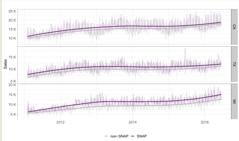
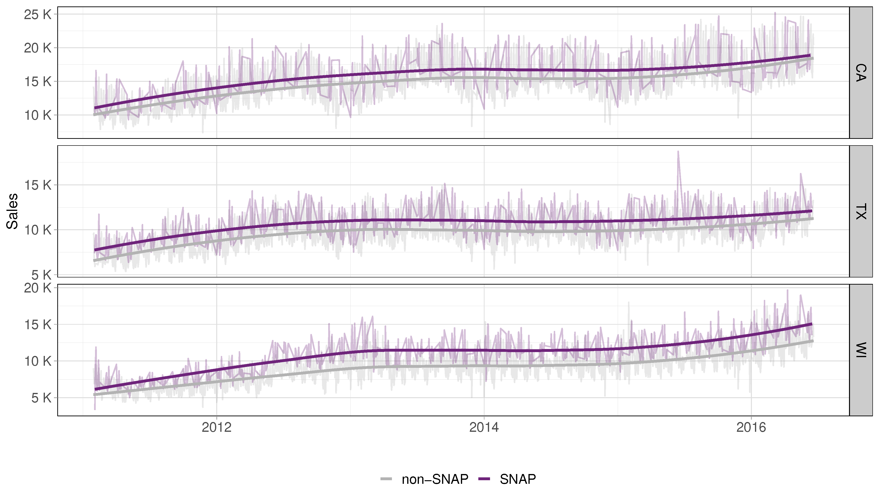
Figure 2 provides a comprehensive overview of the sales volume during SNAP and non-SNAP days in the three states: California, Texas, and Wisconsin. Although the daily time series are visible in the background, it is more informative to examine the smoothed representations. Our analysis shows that sales volumes are significantly higher on SNAP days compared to non-SNAP days in every state. The largest difference is observed in Wisconsin, while the variations over time are relatively minor. Specifically, the two curves in Wisconsin appear to reach their biggest difference around 2013. However, as with all smoothing fits, it is important to exercise caution when examining data at the edges. In such cases, the results may be less reliable and should be interpreted with caution.
We also analyzed sales volumes during special event days versus non-event days in the three states (
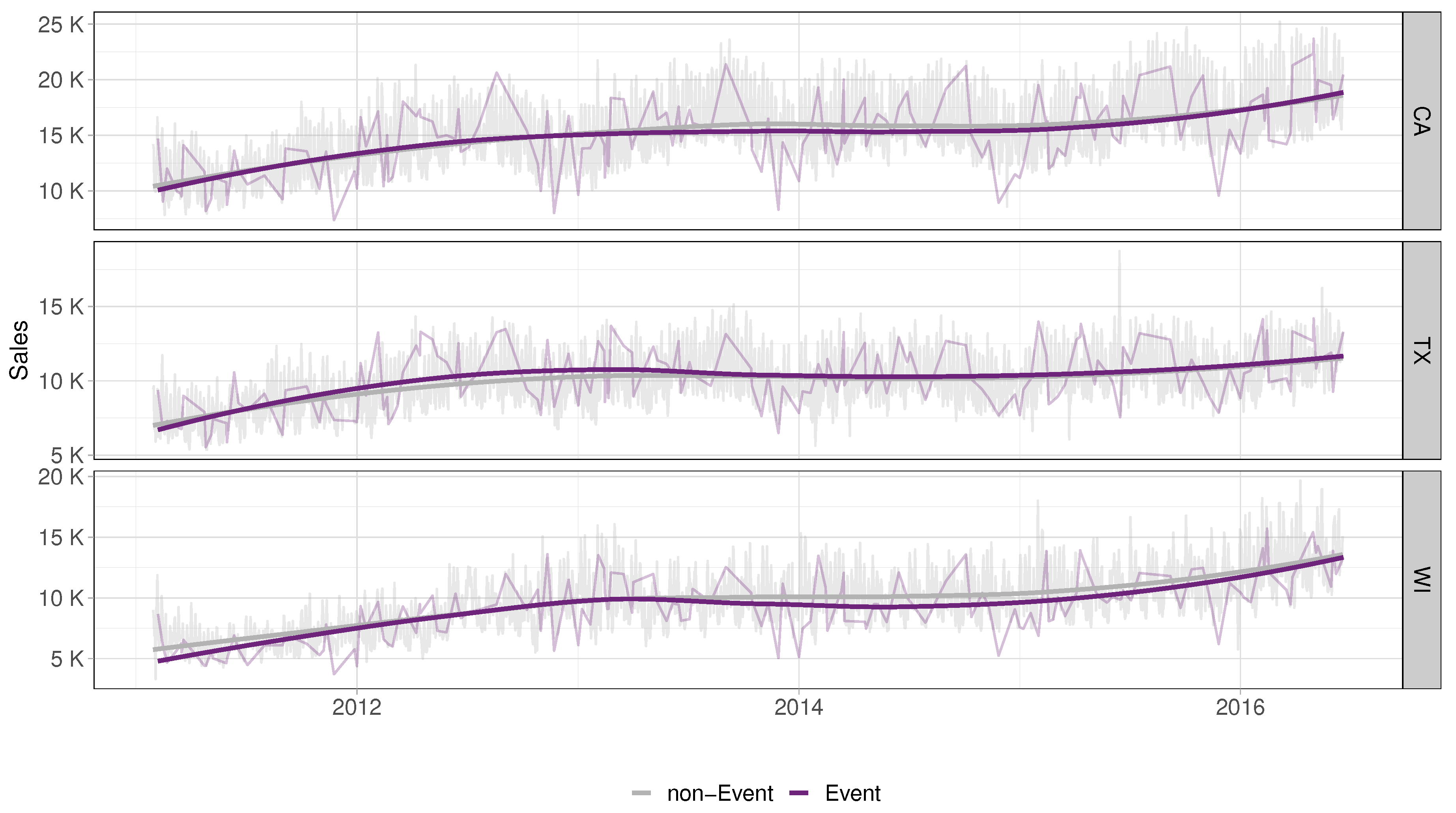
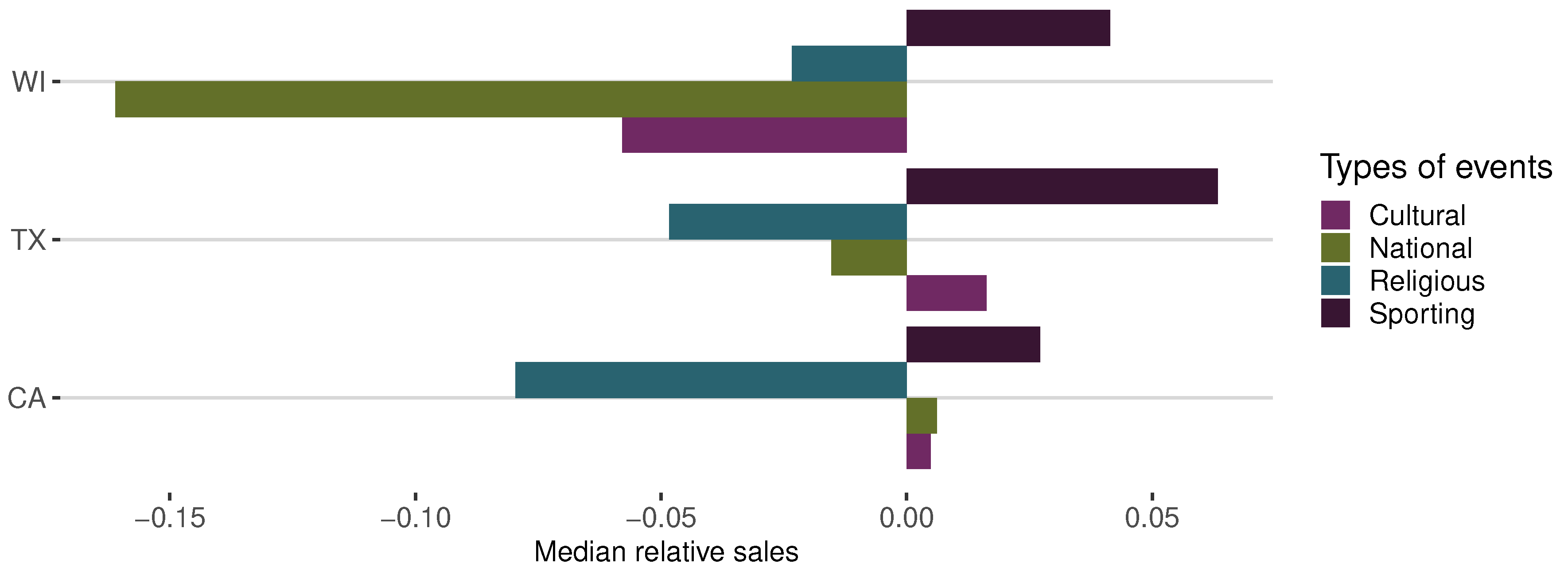
Figure 3). Our findings suggest that special events slightly outsell non-event days in Texas before 2014, while afterward, their sales are similar. In California and Wisconsin, there is a drop in sales around the same time, but here it is from similar sales to lower sales. This pattern appears to be common, starting from 2013. Our analysis of event types is particularly interesting, especially for Wisconsin, where national events result in a considerable adverse effect on sales figures (
Figure 4). Additionally, Wisconsin stands alone as the sole state where cultural events experience lower sales figures, particularly when compared to Texas. On the other hand, religious events show a relatively minor but still unfavorable effect in Wisconsin, while sporting events impacts positively in all three states.
The "Everyday Low Prices" policy has been a key driver of Walmart’s success, helping the company to establish a strong position in the highly competitive retail industry. The idea behind this policy is to provide customers with affordable pricing on a wide range of products throughout the year, rather than relying on the typical retail model of offering higher prices and occasional sales. By maintaining low prices every day, Walmart aims to attract and retain customers who value affordability and reliability in their shopping experience.
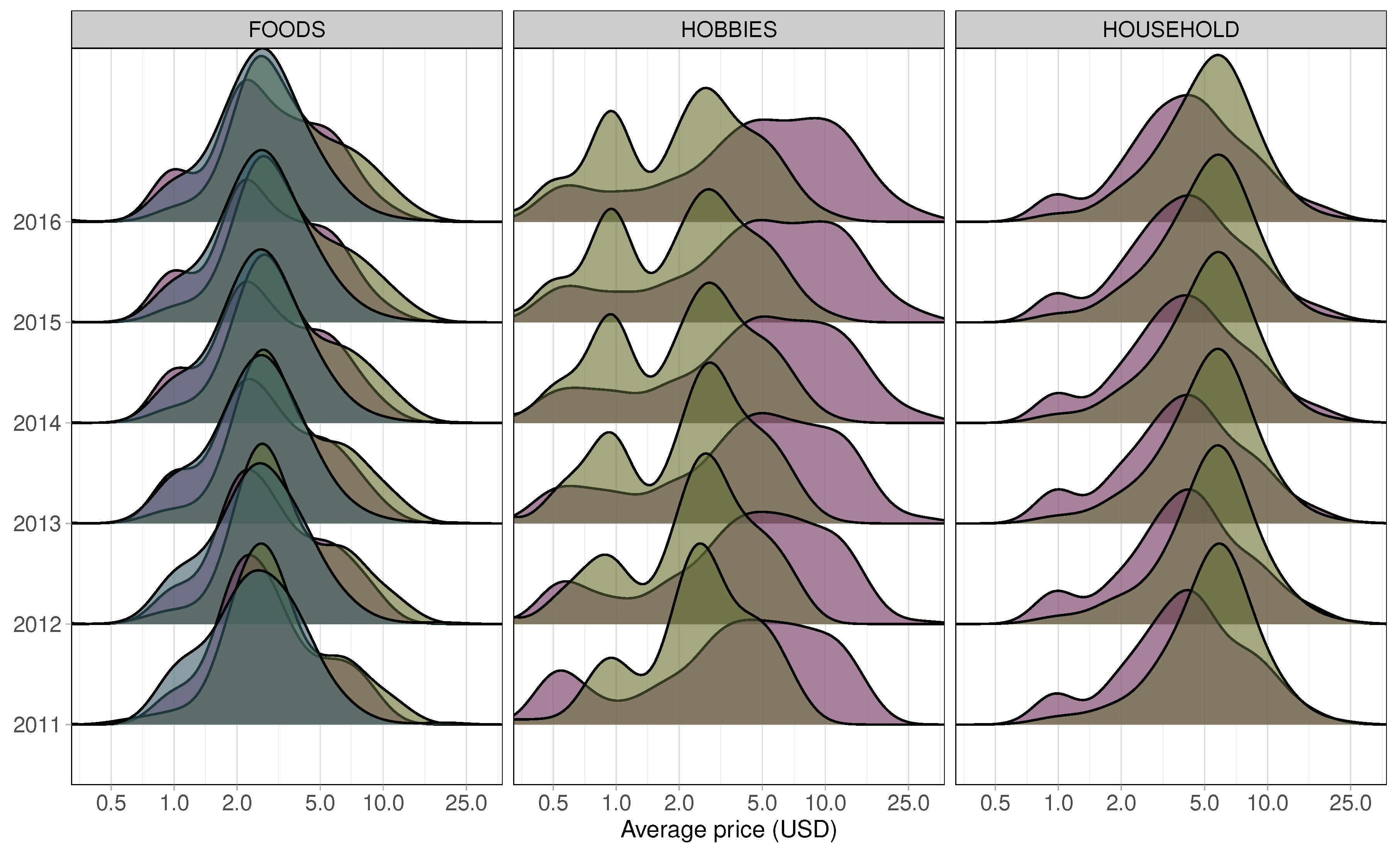
Figure 5 depicts overlapping density plots for weekly average price distributions within each category’s departments for each year from 2011 to 2016. As expected, the price distributions have remained relatively steady, experiencing only slight increases, likely attributed to inflation. However, distinct variations exist among the categories. On average, Foods items tend to be more affordable compared to Household items, whereas Hobbies items exhibit a broader range of prices, even displaying a secondary peak at lower price points. Within each category, there are also substantial differences. For instance, in the Foods category, department 3 (Foods3 in dark green) does not have a high-price tail. The Hobbies category demonstrates the highest diversity, with both departments showing extensive distributions, yet Hobbies1 (in pink) comprises nearly all items priced above 10 USD. Hobbies2 department (in light green) has a bimodal structure. The price distributions in the Household category are quite similar, but Household2 department (in light green) has a peak at clearly higher prices than Household1 department (in pink). An interesting trend is visible in Hobbies2 department, which becomes increasingly bimodal over time. The second peak at 1 USD is growing in importance, almost reaching the level of the main peak just above 2 USD. Meanwhile, the small secondary peak at half a dollar in Hobbies1 department becomes flatter after 2012. Conversely, the Household departments remain very stable, while the Foods category shows small changes such as the relative growth of the 1 USD peak in Foods1 department.
In addition, the M5 dataset includes information about the ID, category, department, store, and state IDs of each item.
3.2. Features engineering
There are two distinct types of features: sequential and categorical. Sequential features are represented as two-dimensional real-valued data, covering both the time and channel dimensions. These sequential features are directly fed into the network without any additional manipulation. On the other hand, categorical features undergo an embedding process before being fed into the network. During this process, the network learns embeddings through an embedding layer, which serves as a lookup table, mapping input values to trainable embeddings [
22].
As a time feature, eight types of values were used: day, month, year, week of the month, week of the year, day of the year, weekday and isweekend. As suggested by [
12], all values were normalized to the range of
. Three normalized price features were utilized, with normalization achieved through a standard score. To obtain this, all values were divided by the standard deviation after the mean value was subtracted. The first normalized price value was obtained for each item across all time, considering disparities from the mean price. The second normalized price value was calculated within each item group that belonged to the same department, allowing for comparisons of the relative price of each item. In each item group associated with the same store, we computed the third normalized price value. This calculation allowed us to make relative price comparisons for each item. We utilized the three values representing the Supplemental Nutrition Assistance Program (SNAP) from the M5 dataset, which is a binary feature indicating whether stores permit SNAP purchases on specific dates, without making any changes to them. The calendar events, characterized by two-dimensional categorical features with varying values based on time, underwent an embedding process before being fed into the network. Regarding the IDs, which are one-dimensional features with constant values regardless of time, we replicated them within the time dimension after embedding, ensuring their dimensions matched with other features.
3.3. Evaluation design
DeepAR global models were trained using the M5 dataset, consisting of 30,490 sales of products across the 10 stores.
The information about the short-term sales trend was derived by using the sales data from the previous 28 days as inputs. We adopted the M5 competition’s framework, where the last 28 days of each time series (from May 23
rd, 2016, to June 19
th, 2016) were reserved as testing set for out-of-sample evaluation. The remaining data, spanning from January 29
th, 2011, to May 22
nd, 2016 (a total of 1941 days), was used for training the models. In order to reach good accuracy results, it is essential to identify a high-performing model during the testing phase. Usually, a validation set is utilized to assess the most appropriate model. The success of a deep learning model is significantly impacted by various factors, including the values for hyperparameters and the values for the initial weights. In order to identify the best model, we used the final 28 days of in-sample training data, covering the period from April 25
th, 2016, to May 22
nd, 2016, as the validation set. The hyperparameter optimization process was carried out using the Optuna optimization framework [
23], with the Root Mean Squared Error (RMSE) [
10] serving as the accuracy metric for model selection. To evaluate the significance of the different types of features, we included them individually and in various combinations, and compared their performance to the baseline case where no features were used.
We assessed the performance of the DeepAR models using two metrics commonly employed in forecasting literature [
24]: the Root Mean Squared Scaled Error (MRMSSE) and the Mean Absolute Scaled Error (MMASE).
Here, is the sales of item i at time t and is its forecast, n is the length of the training set and h is the forecast horizon. In this particular case study, the time frame considered for the forecast horizon is 28 days.
The RMSSE was used as a metric to assess the accuracy of point forecasts in the M5 competition [
25]. MASE and RMSSE are two scale-independent measures that can be used to compare forecasts across different items with different scales and units. This is because they scale the forecast errors based on the MAE or MSE of the 1-step ahead in-sample naïve forecast errors. This ensures that the errors are measured in terms of their absolute or squared magnitude, which allows for fair comparisons across different products. Additionally, MASE and RMSSE differ in how they weight the errors. MASE uses absolute errors, which emphasizes forecasts that closely adhere to the median of the target series. RMSSE uses squared errors, which emphasizes forecasts that closely adhere to the mean of the target series. This difference in weighting allows for different perspectives on the underlying structure of the data.
4. Results and Discussion
The results obtained from the empirical study using DeepAR models on various combinations of features are presented in
Table 1. The Seasonal Naïve model is used as benchmark. This is a simple time series forecasting model that assumes the future value of a series to be equal to the last observed value from the same season. The DeepAR models demonstrate significantly better performance than the local benchmark, as can be observed from the results.
Table 1 highlights the most effective combination in boldface within the MRMSSE and MMASE columns.
Individually, only the features corresponding to IDs improve the baseline model in both performance measures. Including the price features does not improve the model without features, which is not surprising since the prices distributions remain fairly stable over the years. Events improve the baseline model only based on the MMASE, and time features improve the baseline model only based on the MRMSSE. Furthermore, combining the events, time, and price features also does not improve the accuracy of the baseline model, indicating a low relevance of these types of features.
However, when combined with the features corresponding to IDs, the inclusion of events, time, and price features always improves the performance of the former. Interestingly, the best performance is achieved when all the features are used together, suggesting that the individual relevance of each feature is emphasized when the information is given jointly. This model’s performance improved by 1.76% for MRMSSE and 6.47% for MMASE when compared to the model without features.
5. Conclusions
Retailers heavily depend on precise sales forecasts to effectively manage their supply chains and make informed decisions about purchasing, logistics, marketing, finance, and human resources. An advantage of utilizing a global forecasting model, such as an RNN, is its ability to capture intricate dependencies and relationships between different time series. For instance, the sales of a complementary product can affect the sales of another product in a store, or the sales of a particular store can be influenced by the sales at nearby stores. By utilizing a comprehensive model that incorporates all relevant time series, we can more effectively capture these interrelationships and make more precise predictions.
In retail forecasting, covariates such as calendar events, changes in pricing, and weather conditions can be employed to enhance forecast accuracy. The objective of this study was to examine how the accuracy of global forecasting models is influenced by the inclusion of various possible demand covariates, considering their potential impact on operational decision-making. To ensure the significance of our findings, we employed the widely recognized and openly accessible dataset from the M5 competition. We trained DeepAR global models using the complete M5 dataset, which comprises 30,490 product sales across ten stores.
To assess the significance of the different feature types, we included them both individually and in various combinations, comparing their performance against the baseline case where no features were utilized. The findings indicate that, when used individually, only the features corresponding to IDs improved the performance of the baseline model in both performance measures. However, when combined with the features corresponding to IDs, the inclusion of events, time, and price features consistently enhanced the model’s performance. Notably, the optimal performance was achieved when all the features were used in conjunction, indicating that the individual relevance of each feature is accentuated when considered collectively. Overall, the model’s performance demonstrated a 1.76% improvement in MRMSSE and a 6.47% improvement in MMASE compared to the model without features.
Author Contributions
Conceptualization, J.M.O. and P.R.; methodology, J.M.O. and P.R.; software, J.M.O. and P.R.; validation, J.M.O. and P.R.; formal analysis, J.M.O. and P.R.; investigation, J.M.O. and P.R.; resources, J.M.O. and P.R.; data curation, J.M.O. and P.R.; writing—original draft preparation, J.M.O. and P.R.; writing—review and editing, J.M.O. and P.R.; visualization, J.M.O. and P.R.; All authors have read and agreed to the published version of the manuscript.
Funding
This research received no external funding.
Data Availability Statement
Conflicts of Interest
The authors declare no conflict of interest.
References
- Ramos, P.; Santos, N.; Rebelo, R. Performance of state space and ARIMA models for consumer retail sales forecasting. Robotics and Computer-Integrated Manufacturing 2015, 34, 151–163. [Google Scholar] [CrossRef]
- Pinho, J.; Oliveira, J.; Ramos, P. Sales Forecasting in Retail Industry Based on Dynamic Regression Models. In Proceedings of the Advances in Manufacturing Technology XXX; Goh, Y.; Case, K., Eds., Vol. 3, Advances in Transdisciplinary Engineering; 2016; pp. 483–488. [Google Scholar] [CrossRef]
- Ribeiro, C.; Oliveira, J.; Ramos, P. Management of Promotional Activity Supported by Forecasts Based on Assorted Information. In Proceedings of the Advances in Manufacturing Technology XXX; Goh, Y.; Case, K., Eds., Vol. 3, Advances in Transdisciplinary Engineering; 2016; pp. 477–482. [Google Scholar] [CrossRef]
- Ramos, P.; Oliveira, J.M. A procedure for identification of appropriate state space and ARIMA models based on time-series cross-validation. Algorithms 2016, 9, 76. [Google Scholar] [CrossRef]
- Bandara, K.; Hewamalage, H.; Liu, Y.H.; Kang, Y.; Bergmeir, C. Improving the accuracy of global forecasting models using time series data augmentation. Pattern Recognition 2021, 120, 108148. [Google Scholar] [CrossRef]
- Januschowski, T.; Gasthaus, J.; Wang, Y.; Salinas, D.; Flunkert, V.; Bohlke-Schneider, M.; Callot, L. Criteria for classifying forecasting methods. International Journal of Forecasting 2020, 36, 167–177. [Google Scholar] [CrossRef]
- Petropoulos, F.; Apiletti, D.; Assimakopoulos, V.; Babai, M.Z.; Barrow, D.K.; Ben Taieb, S.; Bergmeir, C.; Bessa, R.J.; Bijak, J.; Boylan, J.E.; et al. Forecasting: theory and practice. International Journal of Forecasting 2022, 38, 705–871. [Google Scholar] [CrossRef]
- Ramos, P.; Oliveira, J.; Rebelo, R. Evaluating the Forecasting Accuracy of Pure Time Series Models on Retail Data. In Proceedings of the Advances in Manufacturing Technology XXX; Goh, Y.; Case, K., Eds., Vol. 3, Advances in Transdisciplinary Engineering; 2016; pp. 489–494. [Google Scholar] [CrossRef]
- Wang, Y.; Smola, A.; Maddix, D.; Gasthaus, J.; Foster, D.; Januschowski, T. Deep Factors for Forecasting. In Proceedings of the 36th International Conference on Machine Learning; Chaudhuri, K.; Salakhutdinov, R., Eds. PMLR, 2019, Vol. 97, Proceedings of Machine Learning Research, pp.; pp. 6607–6617.
- Ramos, P.; Oliveira, J.M.; Kourentzes, N.; Fildes, R. Forecasting Seasonal Sales with Many Drivers: Shrinkage or Dimensionality Reduction? Applied System Innovation 2023, 6. [Google Scholar] [CrossRef]
- Oliveira, J.M.; Ramos, P. Assessing the Performance of Hierarchical Forecasting Methods on the Retail Sector. Entropy 2019, 21. [Google Scholar] [CrossRef] [PubMed]
- Salinas, D.; Flunkert, V.; Gasthaus, J.; Januschowski, T. DeepAR: Probabilistic forecasting with autoregressive recurrent networks. International Journal of Forecasting 2020, 36, 1181–1191. [Google Scholar] [CrossRef]
- Rangapuram, S.S.; Werner, L.D.; Benidis, K.; Mercado, P.; Gasthaus, J.; Januschowski, T. End-to-End Learning of Coherent Probabilistic Forecasts for Hierarchical Time Series. In Proceedings of the 38th International Conference on Machine Learning; Meila, M.; Zhang, T., Eds. PMLR, Vol. 139, Machine Learning Research; 2021; pp. 8832–8843. [Google Scholar]
- Rangapuram, S.S.; Kapoor, S.; Nirwan, R.S.; Mercado, P.; Januschowski, T.; Wang, Y.; Bohlke-Schneider, M. Coherent Probabilistic Forecasting of Temporal Hierarchies. In Proceedings of the 26th International Conference on Artificial Intelligence and Statistics; Ruiz, F.; Dy, J.; van de Meent, J.W., Eds. PMLR, Vol. 206, Machine Learning Research; 2023; pp. 9362–9376. [Google Scholar]
- Oliveira, J.M.; Ramos, P. Cross-Learning-Based Sales Forecasting Using Deep Learning via Partial Pooling from Multi-level Data. In Proceedings of the Engineering Applications of Neural Networks; Iliadis, L.; Maglogiannis, I.; Alonso, S.; Jayne, C.; Pimenidis, E., Eds.; Springer Nature Switzerland: Cham, 2023; pp. 279–290. [Google Scholar] [CrossRef]
- Oliveira, J.M.; Ramos, P. Investigating the Accuracy of Autoregressive Recurrent Networks Using Hierarchical Aggregation Structure-Based Data Partitioning. Big Data and Cognitive Computing 2023, 7. [Google Scholar] [CrossRef]
- Alexandrov, A.; Benidis, K.; Bohlke-Schneider, M.; Flunkert, V.; Gasthaus, J.; Januschowski, T.; Maddix, D.C.; Rangapuram, S.; Salinas, D.; Schulz, J.; et al. GluonTS: Probabilistic and Neural Time Series Modeling in Python. Journal of Machine Learning Research 2020, 21, 1–6. [Google Scholar]
- Hochreiter, S.; Schmidhuber, J. Long Short-Term Memory. Neural Computation 1997, 9, 1735–1780. [Google Scholar] [CrossRef] [PubMed]
- Kourentzes, N. Intermittent demand forecasts with neural networks. International Journal of Production Economics 2013, 143, 198–206. [Google Scholar] [CrossRef]
- Zhou, H.; Qian, W.; Yang, Y. Tweedie gradient boosting for extremely unbalanced zero-inflated data. Communications in Statistics - Simulation and Computation 2022, 51, 5507–5529. [Google Scholar] [CrossRef]
- Muhaimin, A.; Prastyo, D.D.; Horng-Shing Lu, H. Forecasting with Recurrent Neural Network in Intermittent Demand Data. In Proceedings of the 11th International Conference on Cloud Computing, Data Science & Engineering (Confluence); 2021; pp. 802–809. [Google Scholar] [CrossRef]
- Jeon, Y.; Seong, S. Robust recurrent network model for intermittent time-series forecasting. International Journal of Forecasting 2022, 38, 1415–1425. [Google Scholar] [CrossRef]
- Akiba, T.; Sano, S.; Yanase, T.; Ohta, T.; Koyama, M. Optuna: A Next-Generation Hyperparameter Optimization Framework. In Proceedings of the 25th ACM SIGKDD International Conference on Knowledge Discovery &, KDD ’19; Data Mining; Association for Computing Machinery: New York, NY, USA, 2019; pp. 2623–2631. [Google Scholar] [CrossRef]
- Hyndman, R.J.; Koehler, A.B. Another look at measures of forecast accuracy. International Journal of Forecasting 2006, 22, 679–688. [Google Scholar] [CrossRef]
- Makridakis, S.; Spiliotis, E.; Assimakopoulos, V. The M5 competition: Background, organization, and implementation. International Journal of Forecasting 2022, 38, 1325–1336. [Google Scholar] [CrossRef]
|
Disclaimer/Publisher’s Note: The statements, opinions and data contained in all publications are solely those of the individual author(s) and contributor(s) and not of MDPI and/or the editor(s). MDPI and/or the editor(s) disclaim responsibility for any injury to people or property resulting from any ideas, methods, instructions or products referred to in the content. |
© 2023 by the authors. Licensee MDPI, Basel, Switzerland. This article is an open access article distributed under the terms and conditions of the Creative Commons Attribution (CC BY) license (http://creativecommons.org/licenses/by/4.0/).
