I. Introduction
The most successful theory, according to the new observation, is Einstein’s theory of general relativity but it has some limitations to explain the phenomenon like the Big Bang singularity, general relativity not respecting local black holes, a consistent quantum gauge field theory of gravity, etc. The data provide compelling evidence that our universe is going through an expansion phase as well as an acceleration phase, according to [
1,
2,
3]. For an understanding of the universe is accelerating in an organized way, from time to time various cosmologists have proposed some well-known modified theories of gravity like
gravity [
4],
gravity [
5,
6,
7],
[
8,
9,
10,
11,
12,
13,
14],
gravity [
15],
gravity [
16],
gravity [
17],
gravity [
18,
19,
20,
21,
22,
23,
24,
25] and recently proposed
[
26,
27,
28,
29,
30] gravity. Dark energy and Dark matter refer back to the unseen additives of the Universe. Dark matter is an invisible, non-baryonic matter believed to give an explanation of phenomena including gravitational lensing and galactic rotation curves. Dark energy is responsible for the accelerating expansion of the Universe [
31,
32].
Geometric variables in symmetric teleparallel gravity reflected the gravitational interaction’s physical characteristics, which are symbolised by the metric’s non-metricity
Q. The non-metricity tensor is the covariant derivative of the metric tensor. This strategy was first presented by Nester and Yo [
18]. The Lagrangian is viewed as an arbitrary function of the non-metricity in an extension of symmetric teleparallel gravity. According to Xu’s gravity theory [
26],
Q and the trace of the matter-energy momentum tensor
T are
. As in
, they cause the cosmos to undergo some large thermodynamic changes [
8].
We are studying various energy conditions in the recently proposed
gravity theory in the present work. Energy conditions play a vital role in defining cosmological evolution, the emergence of Big-Rip Singularities, and Black hole dynamics [
33].It explains how geodesics behave in ways that are similar to space, time, or light. It allows us some latitude in our analysis of particular notions about the nature of cosmic geometries and particular relationships that energy momentum must satisfy under stress in order for energy density to be positive. It is typically used in general relativity to illustrate and investigate space-time singularities [
34]. Using power law in
gravity Capozziello studied the energy condition [
35]. The Null Energy Condition requires for Black hole thermodynamics [
33], whereas the Hawking-Penrose singularity theorem invokes Weak Energy Condition and Strong Energy Condition [
36]. M. Sharif [
37] introduced energy conditions using FLRW universe for two models. The viability of the bounds in
is investigated through energy conditions in [
38]. In different modified theories of gravity like
and generalized teleparallel theory, energy conditions have been investigated [
39,
40,
41,
42].
Motivated from the above analysis and discussion in the present investigation we investigate the two different models in a flat FLRW space-time with proposed equation of state (EoS) , deceleration parameter (q) where p, and represent cosmological pressure, energy density and EoS parameter along with the validation of energy conditions.
The organisation of the analysis is as follows: The fundamental formalism of the
theory of gravity by changing action is presented in
Section II. The gravitational field equations and the emergent scale factor are shown in
Section III.While the empirical constraints that explain model-free parameters are offered in
Section IV. In
Section V cosmological parameters are covered. In
Section VI, a few models of "f(Q,T)" gravity are discussed. We have taken a function
both linear and quadratic as
and
where
,
,
and
are model parameters. A summary of concluding remarks is provided in the last
Section VII.
II. Basic formalism in gravity
The modified Einstein-Hilbert action principle for the
extended symmetric teleparallel gravity is given by [
26]
where
being the general functional form of the non-metricity scalar
Q and the trace of the energy-momentum tensor
T.
g is the determinant of the metric tensor
i.e.
, and
is Lagrangian matter. The non-metricity scalar
Q is defined as
where the deformation tensor
is given by
The non-metricity tensor has the following definition:
and the non-metricity tensor’s trace is derived as
Further, define the super potential tensor as follows
using this the non-metricity scalar is
The variation of the energy-momentum tensor with respect to the metric tensor
read as
where the energy-momentum tensor is
and
Also, the field equations of
gravity are given by varying the action, Equation (
1), with respect to the metric tensor
,
where
,
, and
denotes the covariant derivative. From Equation (
11) it emerge that the field equations of
depend on the tensor
. Various cosmological models of
gravity, depending on the nature of the source of matter are possible. Very recently Koussour et al. [
43] have investigated the quintessence form of extended symmetric teleparallel gravity with cosmic acceleration by assuming the cosmic time-redshift relation as
which gives the Hubble parameter and verify the sustainability of the results through the energy conditions along with jerk parameter. Also, in [
44] the authors investigated energy conditions in
gravity for two different forms of models.
III. Flat FLRW Universe in cosmology
In order to find a solution for the field equations in
extended symmetric teleparallel gravity, some straightforward assumptions, such as the selection of a metric, are frequently required. Consequently, we consider the form’s flat FLRW metric,
where
is the scale factor of the metric and its depends on cosmic time (where unit of the cosmic time is Gyr). Energy-momentum tensor for the Universe, imagine to be behaves like a perfect fluid is given by
Here,
p denotes pressure and
denotes energy density of the Universe. Thus, for tensor
, the expression is obtained as
. The Einstein field equations using the metric (
12) are given as,
Hence overhead
represents a derivative with respect to cosmic time
. In this case,
and
represent differentiation of function
with respect to
Q and
T respectively and
. With the help of Equations (
14) and (
15), the EoS parameter is expressed as
A. Specific Hubble’s parameters and analysis
Now we provide a glimpse on the main features of the scale factor (transit scale factor) and derive a few physical quantities from them to discuss the observed scenario. Hence for the transit scale factor, Hubble’s parameter is observed as
where
,
and
are the model parameters. Keep in mind the relation of
a and
z as
, Equation (
17) becomes
here
represents the present Hubble constant which explains the present expansion rate of the Universe. Freedman et al. [
45] and Suyu et al. [
46] evaluated a value of the present Hubble constant
and
where as recently Plank gives
[
47].
Using the time-redshift differential relation
, the first and second derivative of
H is obtained as
It is interesting to observe and compare our investigated model with the recent observations by finding the best-fit values and the best-fit curve of the Hubble function towards the model parameters , , , and with the recent observational datasets. Hence, here we used the most favorable Hubble and Supernovae SNe-Ia to constrain the said model parameter in the following section.
IV. Observational constraints
The accelerated expansion can be explained by a cosmological constant; alternative explanations, such as dynamical dark energy or modified gravity, can be investigated by looking at how they affect the history of the universe’s late-time expansion or the development of its structures. In order to identify constant parameters, we used the Hubble and Supernova Ia Datasets in this research.
A. Hubble Datasets
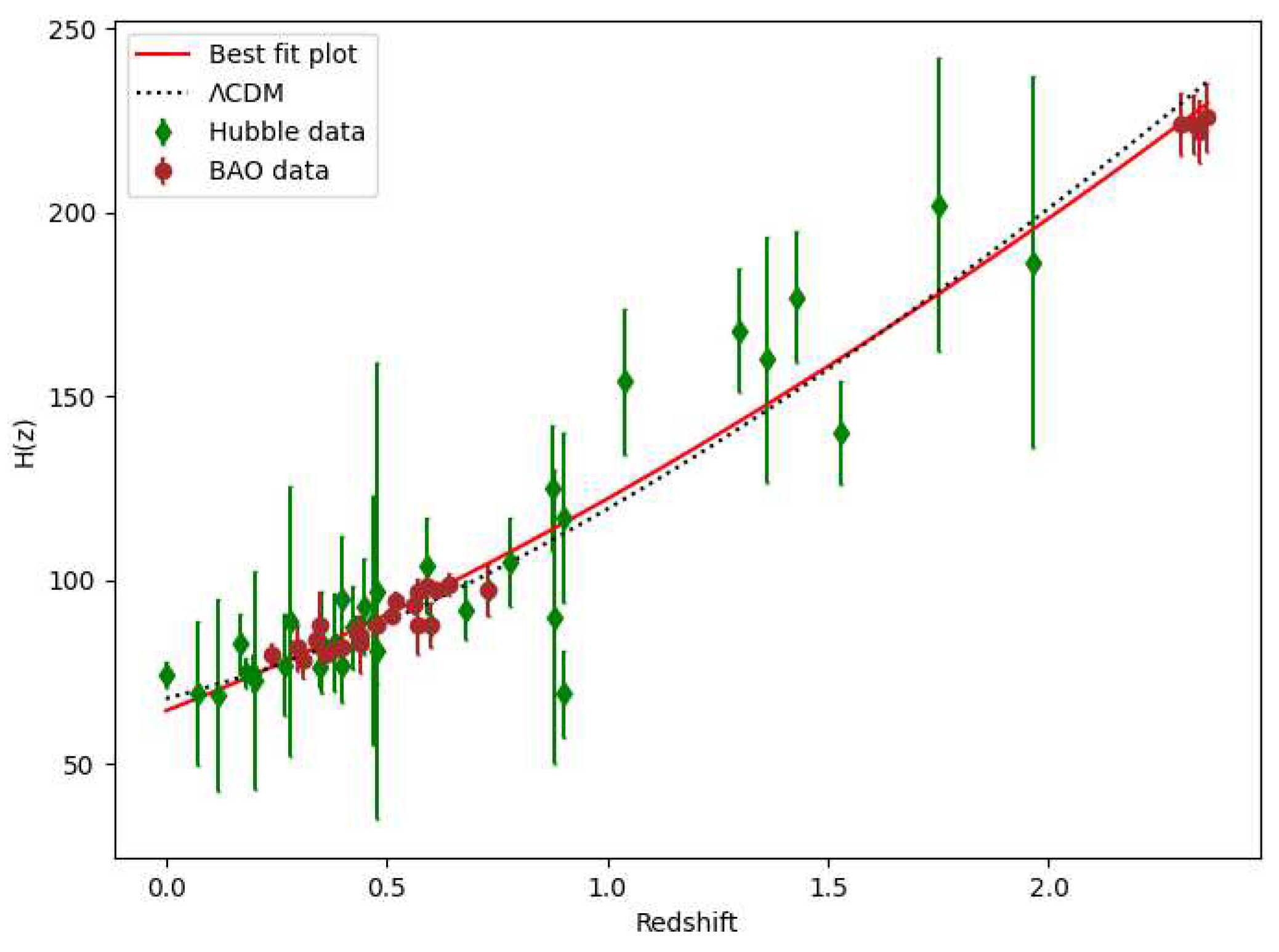
We notice the observational constraints on the parameters , and using the latest 54 data points of in the red-shift range in which 28 points obtained using DA method, whereas 26 points using BAO. The values are presented in Table 2.
We have found best-fit curve of
with 54 data observed values shown in Table 2, using
:
If
shows an exact fit the values of model parameters
,
and
with observational datasets. From Equation (
17) we required
and
. To find the best-fit values of
,
and
we have restricted the parametric space
and
. We used error bars to represent the mean point and its deviation from the mean for 54 points of Hubble data-set and compared our model with the well-accepted
CDM model for
,
and
. We have obtained the best-fit plot for approx values
,
and
having maximum
with RMSE is 11.071 as shows in
Figure 1. Therefore
with
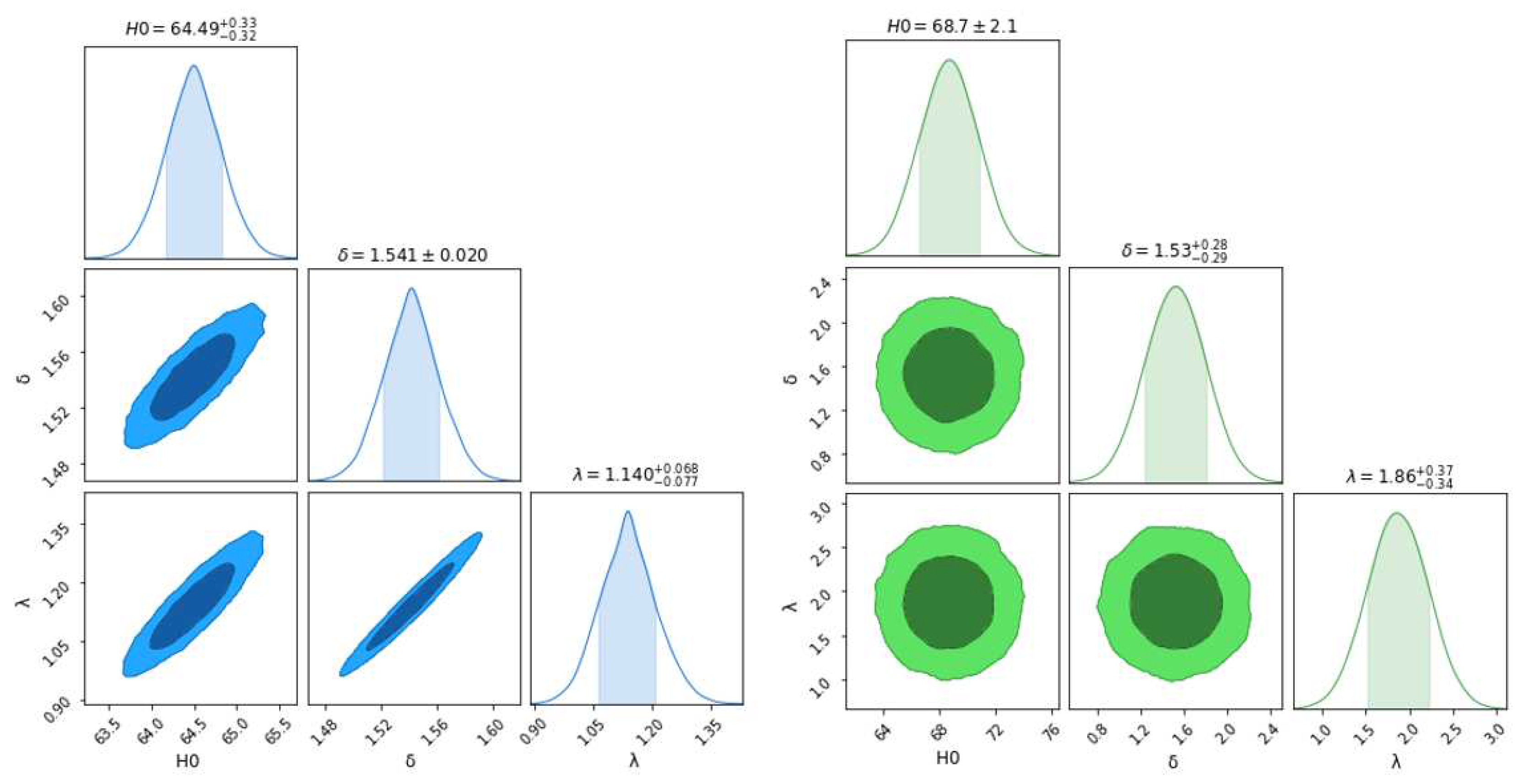
away from exact fit. The Figure 3 show the
(dark blue shaded),
(Sky blue shaded) maximum likelihood contours in the
-
,
-
and
-
planes for Hubble Datasets.
B. Supernovae SNe-Ia
Distance modulus
=
given by
where
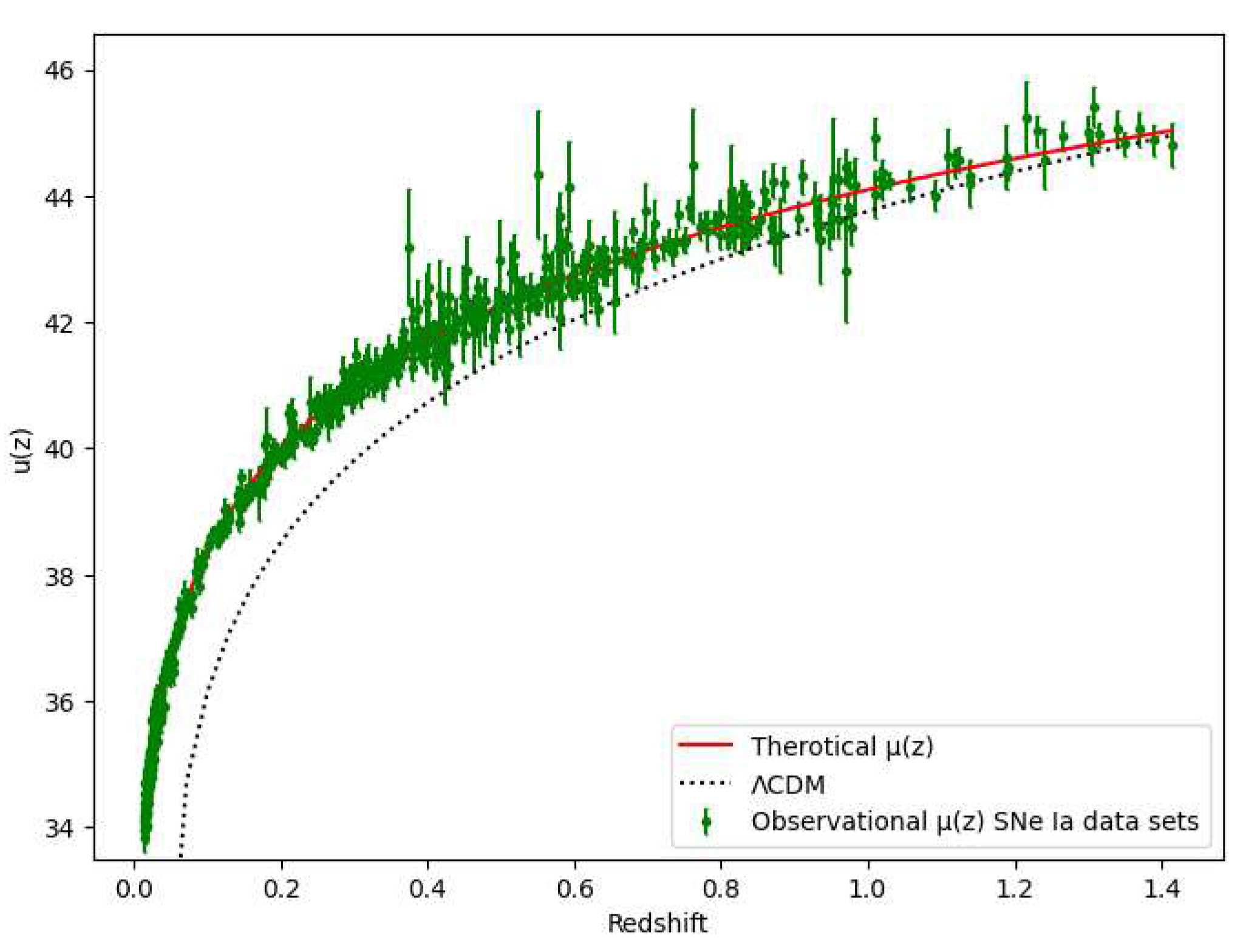
M is constant for all SNe Ia. To obtain the best-fit curve we have to consider data frame having 580 entries observed of apparent magnitude from union 2.1 compilation [
48] where
. From the [
48] statistically significant value of
M is -19.30.
If
shows exact fit the values of model parameters
,
and
with observational datasets. We used error bars to represent the mean point and its deviation from the mean for 580 points of SNe-Ia Dataset and compared our model with the well-accepted
CDM model for
,
and
. We have obtained the best-fit plot for approx values
,
and
having maximum
with RMSE is 0.2662 as shows in
Figure 2.
Therefore
with
away from exact fit. The
Figure 3 show the
(dark green shaded),
(Light green shaded) maximum likelihood contours in the
-
,
-
and
-
planes for SNe-Ia Datasets.
V. Some cosmic parameters and energy conditions
Immediately, we accepted a set of solutions for the planned plan. In order to talk about how Universe is evolved in various phases, we need discuss the behavior of some cosmological parameters like the deceleration parameter, statefinder parameter etc., and these are defined as:
Here the decelerating phase refers to while corresponds to the accelerating phase of the universe. for is the transition point for the Universe from the deceleration to the acceleration phase.
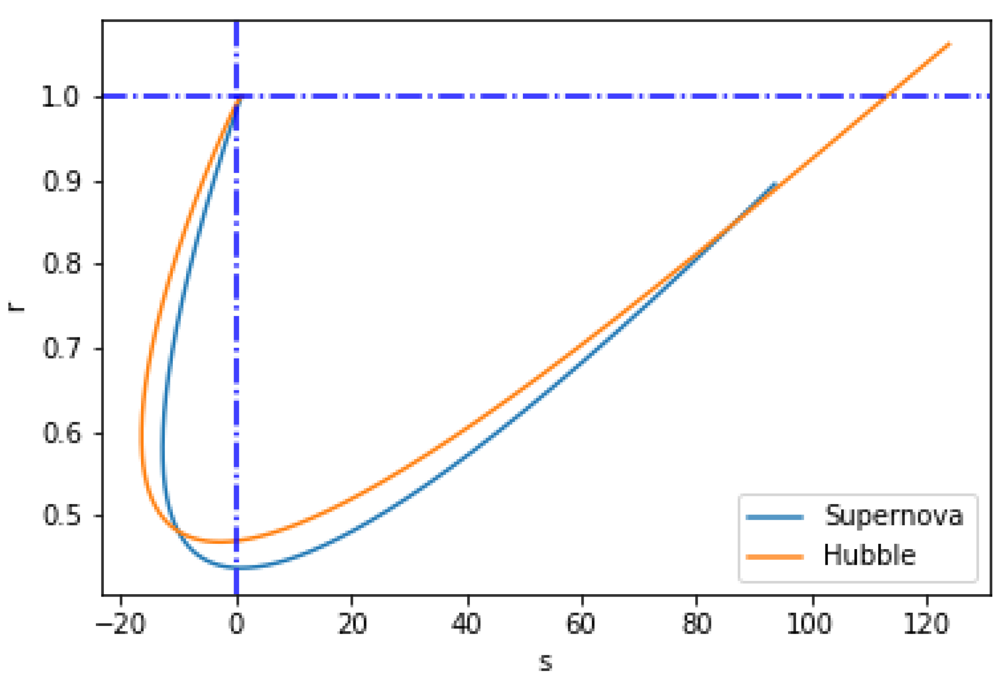
The flat CDM model is shown at the point where the statefinder parameters have the corresponding values. Additionally, keep in mind that in the plane, a positive parameter s (i.e., ) denotes a quintessence-like model of dark energy, whereas a negative parameter s (i.e., ) denotes a phantom-like model of dark energy. Furthermore, by traversing the point , one can evolve from a phantom to the quintessence.
One can derive highly potent and broad theorems regarding the behavior of massive gravitational fields and cosmic geometries using the energy conditions (ECs) of general relativity (GR). Generally speaking, ECs can be divided into
Strong Energy Condition (SEC): Gravity should always be attractive and it formulated as .
Dominant Energy Condition (DEC): When observer measures a matter energy density then will be positive and propagate in a causal way, which leads to .
Weak Energy Condition (WEC): The matter energy density measured by any observer should be positive, .
Null Energy Condition (NEC): It’s the minimum requirement that is implied by SEC and WEC, is .
The violation of the NEC in the energy conditions implies that none of the energy criteria given are valid. The current fast expansion of the universe has raised questions about the SEC. In cosmological situations during the inflationary expansion and at the present, SEC must be broken.
Making use of Equations (
18) and (
19), the deceleration parameter and statefinder parameters are obtained as
After analysing the SNe-Ia data by many researchers it was observed that datasets favour current acceleration for
and past deceleration for
. A little while back, according to the high-z supernova search (HZSNS) team
at (1
) confidence level [
49] which has been further analyzed to
at (1
) [
49]. According to SNLS [
50], as well as the one recently compiled in [
51], the transition red-shift
≡ 0.6 (1
) is in better agreement with the flat
CDM model
. Another limit is
(2
, joint analysis) [
52]. Further, the transition red-shift for our derived model comes to be
for observed Hubble datasets and
for supernovae which is in best agreement with the SNe- Ia supernovae observations, including the farthest known supernova SNI997ff at
[
53]. We see that the variation of
q with
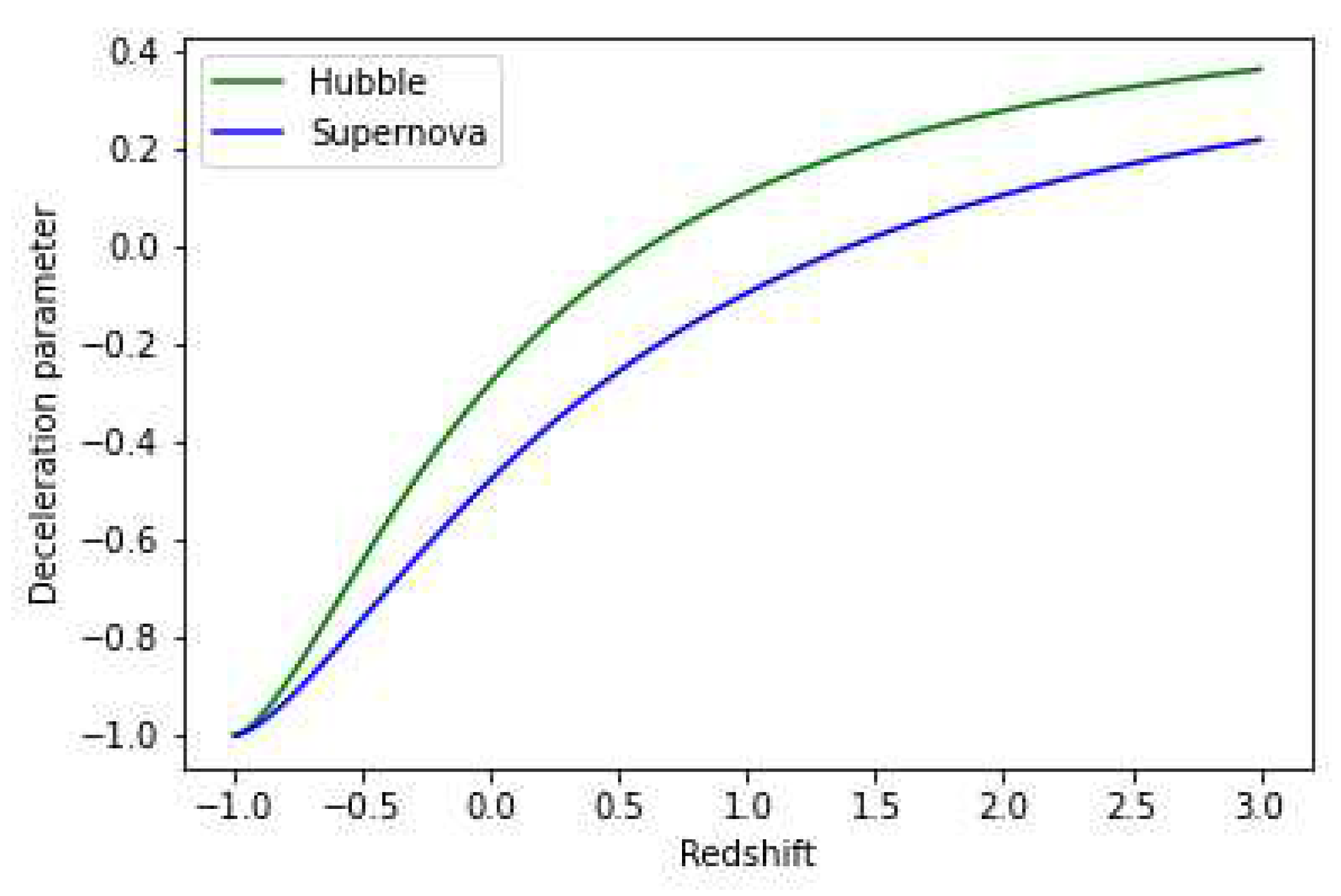
z obtained in our model is compatible with the results. In our derived model the best-fit value of deceleration parameter
for Hubble and Supernova is -0.2792 , -0.4774.
Figure 4 shows plot of deceleration parameter v Redshift for both Hubble and Supernovae datasets for values of model parameters
,
and
are from
Table 1.
In this study, it was argued that
plane is useful to differentiate between various models. An analysis based on
has also useful to differentiate between general relativity and modified theory of gravity. We note that for the Hubble datasets, the
r and
s parameters at the present epoch are
and
while for the SNe-Ia datasets,
and
as shown in
Figure 5. Currently, observations are not sensitive enough to measure these parameters. Future data, however, could be used to infer these values, which would tremendously aid in defining the characteristics of dark energy.
VI. Models of gravity
In this section, we discuss some physical aspects of different models of gravity
A. Model-I
Here we consider the
gravity model as
For above model the field Equations (
14)–(
16), take the form
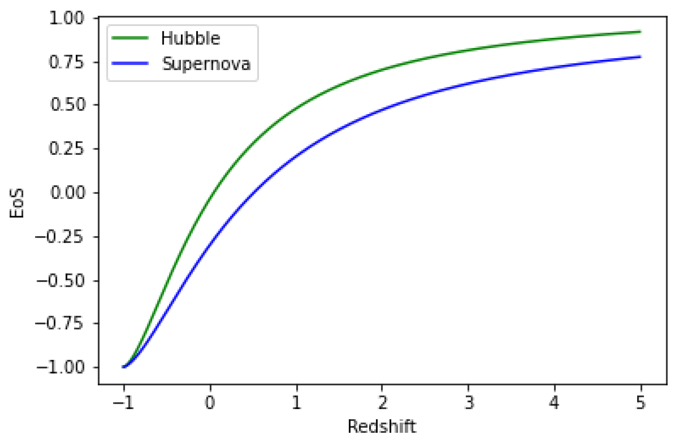
Figure 6 shows a plot of Pressure versus Redshift for both Hubble and SNe-Ia datasets for
,
and
are from
Table 1 while model parameters
=-0.0125 and
=-0.012 respectively.
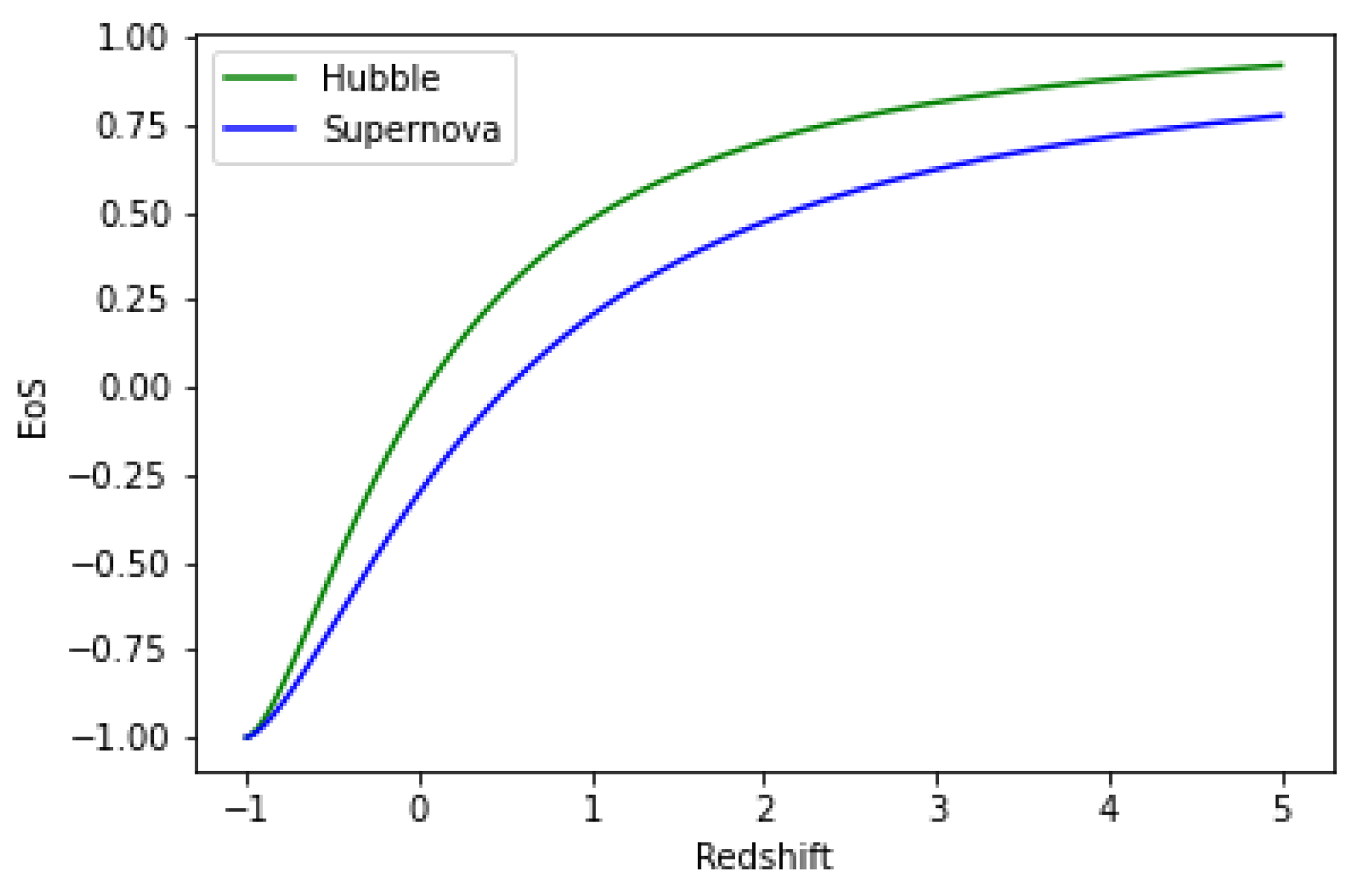
The EoS parameter is associated with energy density and pressure p. The EoS parameter appears to be positive in the beginning. As a consequence, it moves from the positive region to negative region. The negative is proposed a constant vacuum energy density, It’s worth noting that shows Pressure-less Cold matter (PCL), represents Hot matter, is radiation, is Hard Universe, shows stiff fluid (SF), is Ekpyrotic matter (Ek-M), stand for the quintessence (Q) region and stands for the phantom region (Ph) , respectively while represents the cosmological constant ( CDM) and is precluded by SNe-Ia perceptions. Subsequently, the evolving range of of our derived model is supportive of ( CDM) model in both Hubble and supernova data.
From
Figure 7, we can observe that the Universe exists the decelerated regime and enters in the accelerating phase as studied [
54].
Furthermore, to verify the genuineness of model in context of cosmic acceleration, we resolve different forms of energy conditions by calculating
and
for NEC, DEC and SEC respectively.
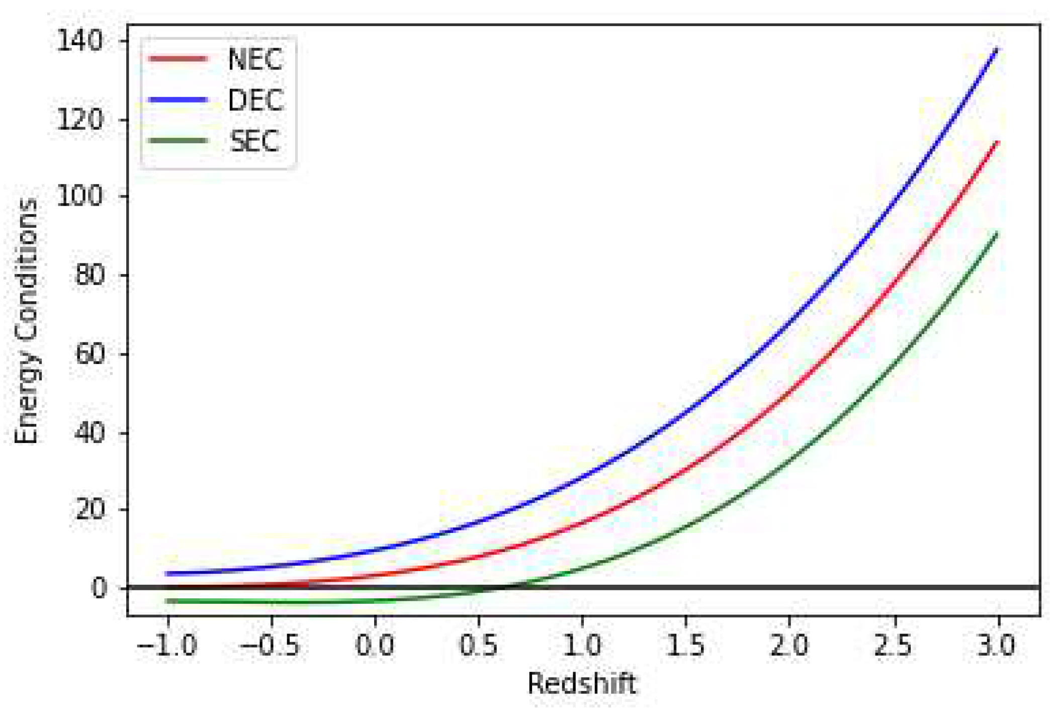
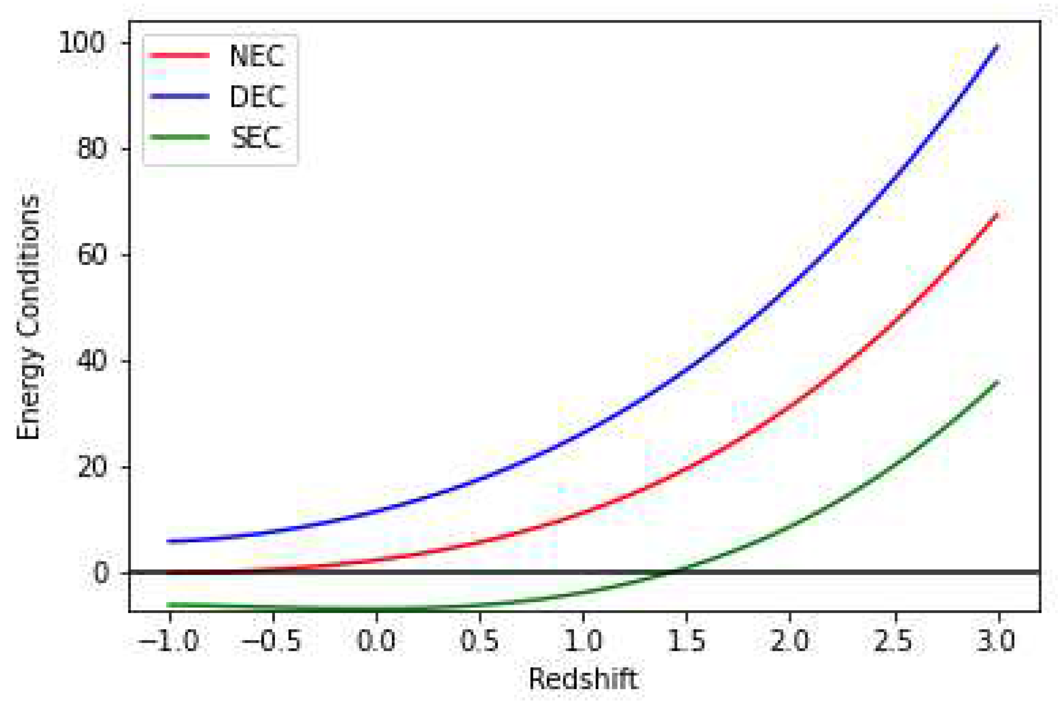
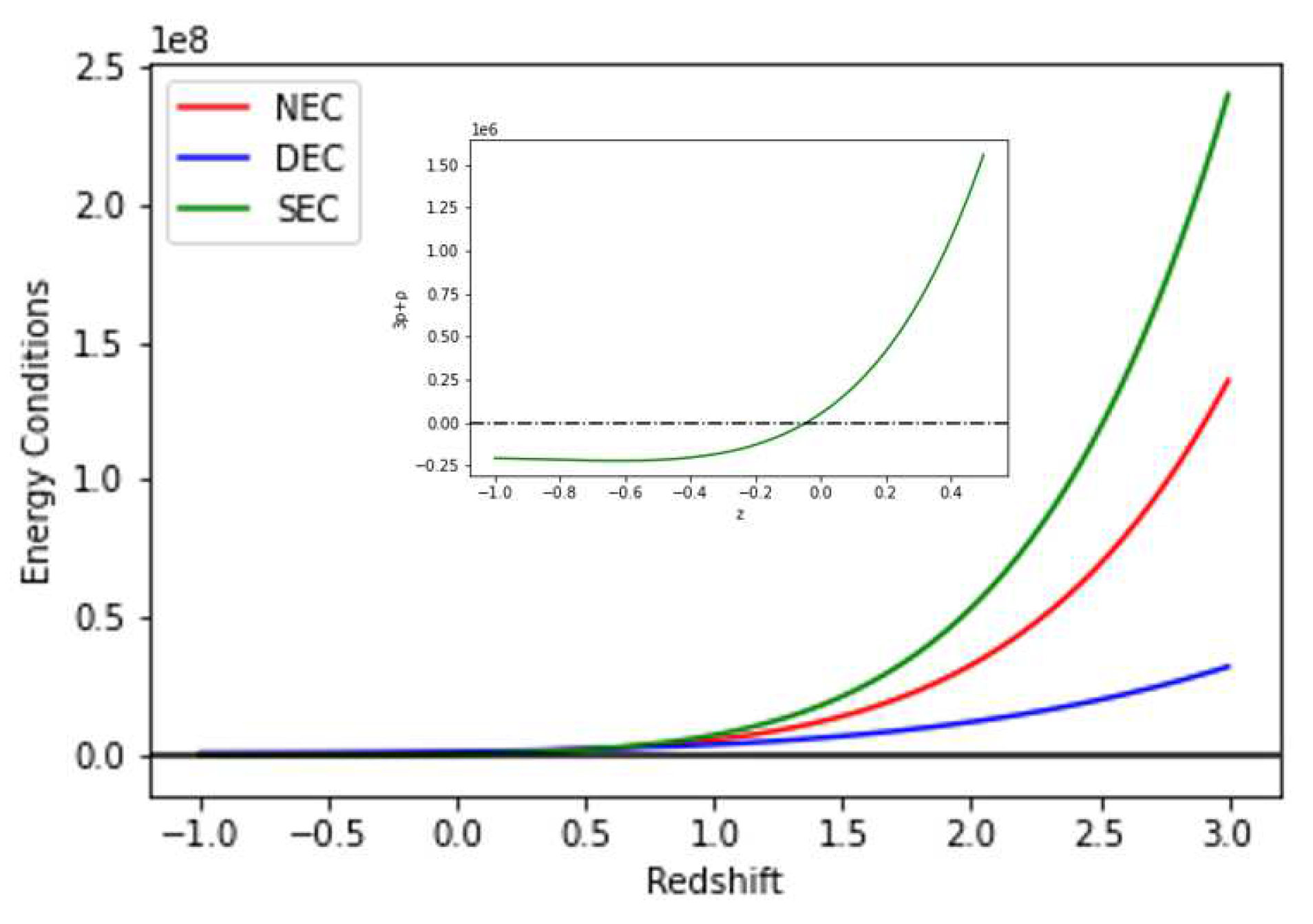
Figure 8 and
Figure 9 are plots of Energy Conditions with respect to constant obtained from best-fit for Hubble and SNe-Ia datasets as shown in
Table 1 and model parameters
=-0.0125 and
=-0.012. According to the both data of the accelerating Universe, the SEC must be violated on cosmological scale [
55,
56]. Also, negative EoS (
) indicate that
. Therefore, there is a violation of the SEC at present. We also can see in
Figure 8 and
Figure 9 that the NEC, and DEC are obeying for both Hubble and SNe-Ia datasets. Since we have shown the behavior of energy density in
Figure 6. We have examined the NEC behavior (i.e., partial condition of WEC). Therefore, validation of NEC and energy density together results in the validation of WEC.
Table 2.
54 points of data: 28 (DA) + 26 (BAO+other).
Table 2.
54 points of data: 28 (DA) + 26 (BAO+other).
| z |
H(z) |
|
Ref. |
z |
H(z) |
|
Ref. |
| 0.07 |
69 |
19.6 |
[57] |
0.9 |
69 |
12 |
[58] |
| 0.120 |
68.6 |
26.2 |
[57] |
0.170 |
83 |
8 |
[59] |
| 0.179 |
75 |
4 |
[60] |
0.2 |
72.9 |
29.6 |
[57] |
| 0.27 |
77 |
14 |
[59] |
0.28 |
88.8 |
36.6 |
[57] |
| 0.350 |
76.3 |
5.6 |
[61] |
0.38 |
83 |
13.5 |
[62] |
| 0.4 |
95 |
17 |
[59] |
0.42 |
87.1 |
11.2 |
[62] |
| 0.44 |
92.8 |
12.9 |
[62] |
0.47 |
89 |
34 |
[57] |
| 0.48 |
97 |
62 |
[63] |
0.6 |
87.9 |
6.1 |
[64] |
| 0.68 |
92 |
8 |
[60] |
0.73 |
97.3 |
7 |
[64] |
| 0.78 |
105 |
12 |
[60] |
0.87 |
125 |
17 |
[60] |
| 0.90 |
117 |
23 |
[59] |
1.037 |
154 |
20 |
[60] |
| 1.3 |
168 |
17 |
[59] |
1.363 |
160 |
33.6 |
[59] |
| 1.430 |
177 |
18 |
[59] |
1.530 |
140 |
14 |
[59] |
| 1.750 |
202 |
40 |
[59] |
1.965 |
186.5 |
50.4 |
[65] |
| 0.24 |
79.69 |
2.99 |
[66] |
0.30 |
81.7 |
6.22 |
[67] |
| 0.31 |
78.18 |
4.74 |
[68] |
0.34 |
83.8 |
3.66 |
[66] |
| 0.35 |
87.7 |
9.1 |
[69] |
0.36 |
79.94 |
3.38 |
[68] |
| 0.38 |
81.5 |
1.9 |
[70] |
0.40 |
82.04 |
2.03 |
[68] |
| 0.43 |
86.45 |
3.97 |
[66] |
0.44 |
82.6 |
7.8 |
[71] |
| 0.44 |
84.81 |
1.83 |
[68] |
0.48 |
87.79 |
2.03 |
[68] |
| 0.51 |
90.4 |
1.9 |
[70] |
0.52 |
94.35 |
2.64 |
[68] |
| 0.56 |
93.34 |
2.3 |
[68] |
0.57 |
87.6 |
7.8 |
[72] |
| 0.57 |
96.8 |
3.4 |
[73] |
0.59 |
98.48 |
3.18 |
[68] |
| 0.6 |
87.9 |
6.1 |
[71] |
0.61 |
97.3 |
2.1 |
[70] |
| 0.64 |
98.82 |
2.98 |
[68] |
0.73 |
97.3 |
7 |
[71] |
| 2.30 |
224 |
8.6 |
[74] |
2.33 |
224 |
8 |
[75] |
| 2.34 |
222 |
8.5 |
[76] |
2.36 |
226 |
9.3 |
[77] |
B. Model-II
Here we consider the
gravity model as,
For above model the field Equations (
14)–(
16), take the form
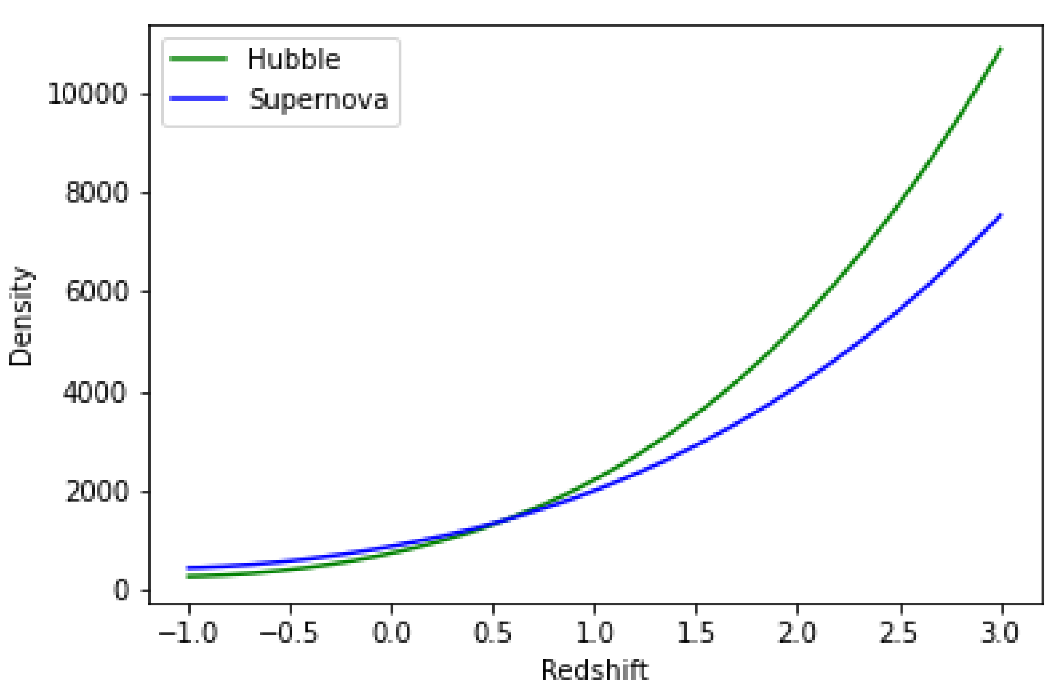
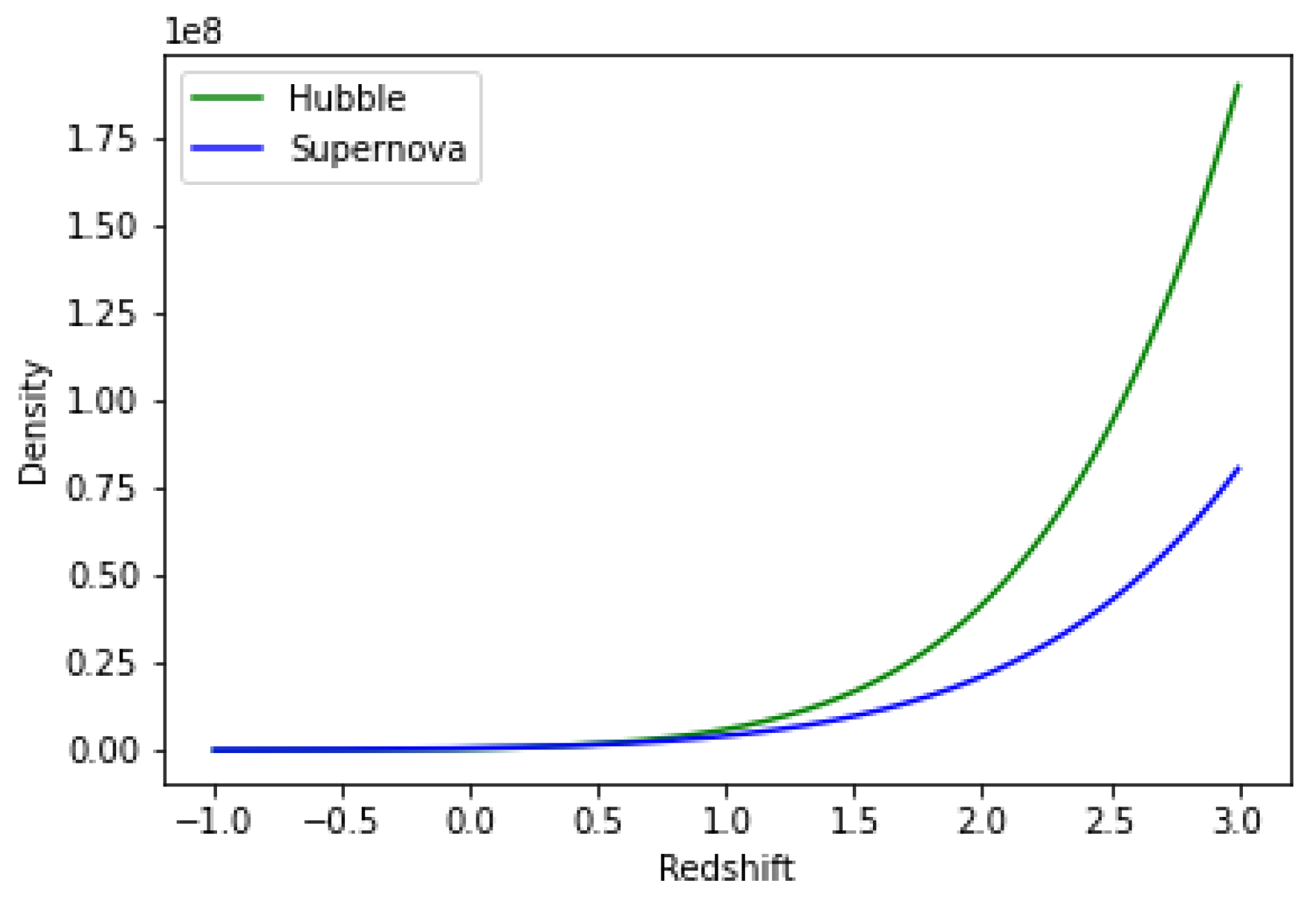
Figure 10 shows plot of Density versus redshift for both Hubble and SNe-Ia datasets for
,
and
are from Table 1, while model parameters
=-0.0125 and
=-0.012 respectively.
As shown in
Figure 11, the universe is in an accelerating mode and is about to enter a decelerating phase. Additionally, we resolve various energy conditions by calculating the model’s accuracy in the context of cosmic acceleration.
and
for NEC, DEC and SEC, respectively.
For NEC, DEC and SEC respectively.
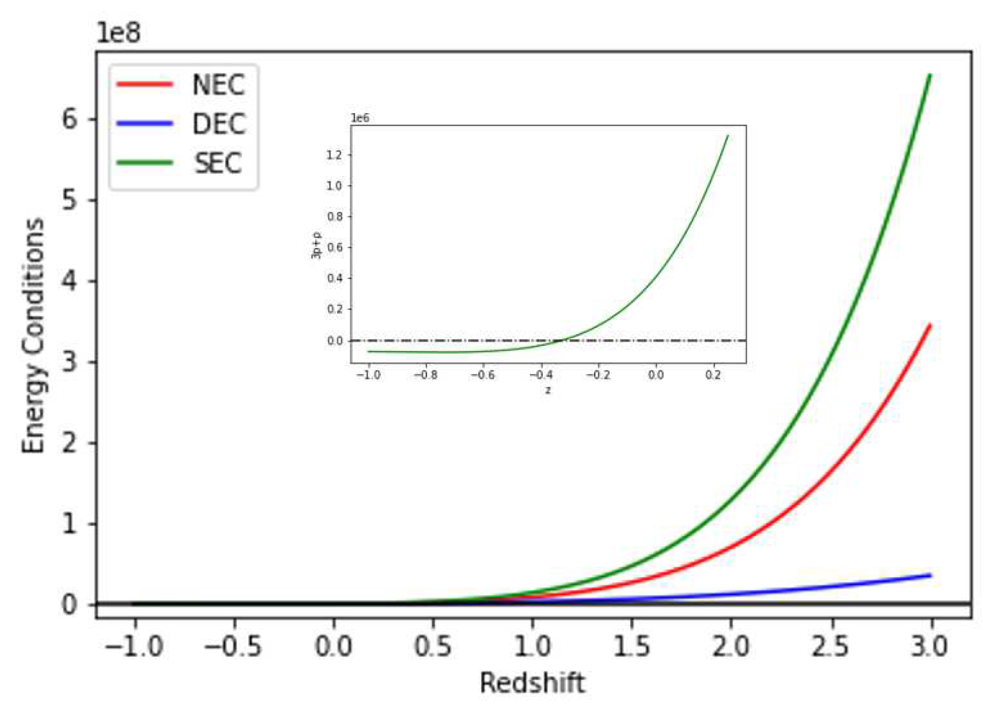
Figure 12 and
Figure 13 are plots of Energy Conditions with respect to constant obtained from best-fit for Hubble and SNe-Ia datasets as shown in
Table 1 and model parameters
=-0.0125 and
=-0.012. According to the both data of the accelerating Universe,as shown in
Figure 12 and
Figure 13 the SEC must be violated on cosmological scale [
55,
56]. Also, negative EoS (
) indicate that
. Therefore, there is a violation of the SEC at present.
Figure 12 and
13 indicate that the NEC, and DEC are obeying for both Hubble and SNe-Ia datasets. We have examined the NEC behavior (i.e., partial condition of WEC). Therefore, validation of NEC and energy density together results in the validation of WEC.
VII. CONCLUSIONS
In present work we have taken a function
both linear and quadratic as
where
,
,
and
are model parameters. In terms of redshift
z, we have measured a number of cosmological parameters in the FLRW universe, including the Hubble parameter
H and the deceleration parameter
q. By applying the
formula for observational constraints on the model, we were able to determine the approximate best-fit values of the model parameters
utilizing datasets like the Hubble data set
and union 2.1 compilation of SNe-Ia datasets. The current values of the cosmological models
and
that we estimated are close to the values found in mainstream cosmology. Talk about EoS and the various energy conditions. Following are the characteristics of our cosmological model:
Figure 1 and
Figure 2 provide best-fit plots based on the observed datasets. For the best fit, we employed a hybrid model combining the gradient descent and least squares approach.
-value for Hubble and SNe-Ia datasets are
and
respectively. SNe-Ia has 580 observation and giving best-fit among both datasets.
Hubble function derived is constrained by observational datasets i.e. Hubble and SNe-Ia datasets and the present value of Hubble constant is and respectively with respect to best-fit plot.
The transition from early deceleration to the universe’s present acceleration is shown by the deceleration parameter and with respect to Hubble and SNe-Ia datasets.
We have considered two functional form of gravity in Section A, Section B and watched how the energy density and EoS parameter all behaved. The EoS parameter exhibits a transition from early deceleration to late time acceleration with regard to the model parameters, while the density in both models exhibits positive behavior.
In both the functional form of
of Section A and Section B, NEC, WEC and DEC are satisfied whereas SEC is violated (see
Figure 8,
Figure 9,
Figure 12 and
Figure 13).
Data Availability Statement
No advanced data associated with this article.
Acknowledgments
The IUCAA, Pune, India, provided the facilities and support under the Visiting Associateship Programmes, for which the authors (S. H. Shekh and A. Pradhan) are grateful.
Conflicts of Interest
The authors declared that they have neither personal relationships nor competing financial interests that could influenced the work reported in this paper.
References
- Perlmutter, S.; Aldering, G.; Goldhaber, G.; Knop, R.A.; Nugent, P.; Castro, P.G.; Deustua, S.; Fabbro, S.; Goobar, A.; Groom, D.E.; et al. Measurements of Ω and Λ from 42 high-redshift supernovae. Astrophys. J. 1999, 517, 565–586. [Google Scholar] [CrossRef]
- Kamenshchik, A.Y.; Tronconi, A.; Venturi, G. Dynamical dark energy and spontaneously generated gravity. Phys. Lett. B 2012, 713, 358–364. [Google Scholar] [CrossRef]
- Sahni, V.; Starobinsky, A. Reconstructing dark energy. Int. Jour. Mod. Phys. D 2006, 12, 2105–2132. [Google Scholar] [CrossRef]
- Nojiri,S. ; Odintsov, S.D.; Sasaki, M. Gauss-Bonnet dark energy. Phys. Rev. D 2005, 71, 123509. [Google Scholar]
- Buchdahl, H. A. Non-linear Lagrangians and cosmological theory, Monthly Not. Roy. Astron. Soc. 1970, 150, 1–8. [Google Scholar] [CrossRef]
- Dixit, A.; Bhardwaj, V.K.; Pradhan, A.; Krishnannair, S. Observational constraint in Kantoswki-Sachs f(R) gravity model with strange quark matter. Indian J. Phys. 2023. [Google Scholar] [CrossRef]
- Debnath, U.; Molla, N.U.; Pradhan, A. Noncommutative wormhole in non-minimal curvature-matter coupling of f(R) gravity with Gaussian and Lorentzian distributions. Int. J. Geom. Methods Mod. Phys. 2023. [Google Scholar] [CrossRef]
- Harko, T.; Lobo, F.S.; Nojiri, S.I.; Odintsov, S.D. f (R, T) gravity. Phys. Rev. D 2011, 84, 024020. [Google Scholar] [CrossRef]
- Tangphati, T.; Panotopoulos, G.; Banerjee, A.; Pradhan, A. Charged compact stars with colour-flavour-locked strange quark matter in f(R,T) gravity. Chin. J. Phys. 2023, 82, 62–74. [Google Scholar] [CrossRef]
- Pradhan, A.; Goswami, G.K.; Beesham, A. The reconstruction of constant Jerk parameter with f(R,T) gravity. Jour. High Energy Astrophys. 2023, 38, 12–21. [Google Scholar] [CrossRef]
- Pradhan, A.; Goswami, G.K.; Beesham, A. The reconstruction of constant Jerk parameter with f(R,T) gravity in Bianchi-I spacetime. Europ. Phys. J. Plus 2023, 138, 451. [Google Scholar] [CrossRef]
- Pradhan, A.; Goswami, G.K.; Beesham, A. Reconstruction of an observationally constrained f(R,T) gravity model. Int. J. Geom. Methods Mod. Phys. 2023, 2350169. [Google Scholar] [CrossRef]
- Pradhan, A.; Goswami, G.K.; Beesham, A. An f(R, T) gravity based FLRW model and observational constraints. Astronomy and Computing, 2023, 44, 100737. [Google Scholar] [CrossRef]
- Zubair, M.; Zeeshan, M.; Hasan, S.S.; Oikonomou, V.K. Impact of collisional matter on the late-time dynamics of f(R,T) gravity. Symmetry 2018, 10, 463. [Google Scholar] [CrossRef]
- Cai, Y.F.; Capozziello, S.; De Laurentis, M.; Saridakis, E.N. f (T) teleparallel gravity and cosmology. Rep. Prog. Phys. 2016, 79, 106901. [Google Scholar] [CrossRef]
- Sharif, M.; Ikram, A. Energy conditions in f (G, T) gravity, Eur. Phys. J. C 2016, 76, 640. [Google Scholar]
- Ayuso, I.; Jimenez, J.B.; Cruz-Dombriz, A. Consistency of universally nonminimally coupled f(R,T,RμνTμν) theories. Phys. Rev. D 2013, 91, 104003. [Google Scholar] [CrossRef]
- Nester, J.M.; Yo, H.J. Symmetric teleparallel general relativity. Chin. J. Phys. 1999, 37, 113. [Google Scholar]
- Pradhan, A.; Maurya, D.C.; Dixit, A. Dark energy nature of viscous Universe in f(Q)-gravity with observational constraints. Int. J. Geom. Method Mod. Phys. 2021, 18, 2150124. [Google Scholar] [CrossRef]
- Banerjee, A.; Pradhan, A.; Tangphati, T.; Rahaman, F. Wormhole geometry in f(Q) gravity and the energy conditions. Europ. Phys. J. C 2021, 81, 10131. [Google Scholar] [CrossRef]
- Dixit, A.; Maurya, D.C.; Pradhan, A. Phantom dark energy nature of bulk-viscosity universe in modified f(Q)-gravity. Int. J. Geom. Methods Mod. Phys. 2022, 19, 2250198. [Google Scholar] [CrossRef]
- Pradhan, A.; Dixit, A.; Maurya, D.C. Quintessence behaviour of an anisotropic bulk viscous cosmological model in modified f(Q)-gravity. Symmetry 2022, 14(12), 2630. [Google Scholar] [CrossRef]
- Gupta, S.; Dixit, A.; Pradhan, A. Tsallis holographic dark energy scenario in viscous F(Q) gravity and Tachyon field. Int. J. Geom. Methods Mod. Phys. 2023, 20, 2350021. [Google Scholar] [CrossRef]
- Shekh, S.H.; Bouali, A.; Mustafa, G.; Pradhan, A. Observational constraints in accelerated emergent f(Q) gravity model. Class. Quantum Grav. 2023, 40, 0555011. [Google Scholar] [CrossRef]
- Maurya, D.C.; Dixit, A.; Pradhan, A. Transit string dark energy models in f(Q) gravity. Int. J. Geom. Methods Mod. Phys. 2023, 20, 2350134. [Google Scholar] [CrossRef]
- Xu, Y.; Li, G.; Harko, T.; Liang, S. f(Q, T) gravity. Eur. Phys. J. C 2019, 79, 708. [Google Scholar] [CrossRef]
- Pradhan, A.; Dixit, A. The model of the transit cosmology along with observational constrictions in f(Q,T) gravity. Int. J. Geom. Method Mod. Phys. 2021, 18, 2150159. [Google Scholar] [CrossRef]
- Shekh, S.H.; Bouali, A.; Pradhan, A.; Beesham, A. New emergent observational constraints in f(Q,T) gravity model. Jour. High Energy Astrophys. 2023, 39, 53–59. [Google Scholar] [CrossRef]
- Xu, Y.; Harko, T.; Shahidi, S.; Liang, S. Weyl type f(Q, T) gravity, and its cosmological implications. Eur. Phys. J. C 2020, 80, 449. [Google Scholar] [CrossRef]
- Narawade, S.A.; Koussour, M.; Mishra, B. Constrained f(Q,T) gravity accelerating cosmological model and its dynamical system analysis. Nucl. Phys. B 2023, 992, 116233. [Google Scholar] [CrossRef]
- Riess, A.G.; Macri, L.; Casertano, S.; Lampeitl, H.; Ferguson, H.C.; Filippenko, A.V.; Jha, S.W.; Li, W.; Chornock, R. A 3% solution: determination of the Hubble constant with the Hubble Space Telescope and Wide Field Camera 3. Astrophys. J. 2011, 730, 119. [Google Scholar] [CrossRef]
- Riess, A.G.; Filippenko, A.V.; Challis, P.; Clocchiatti, A.; Diercks, A.; Garnavich, P.M.; Gilliland, R.L.; Hogan, C.J.; Jha, S.; Kirshner, R.P.; Leibundgut, B.R.U.N.O. Observational evidence from supernovae for an accelerating universe and a cosmological constant. Astro. J. 1998, 116, 1009. [Google Scholar] [CrossRef]
- Hawking, S.W.; Ellis, G.F.R. The large scale structure of space-time. Cambridge University Press ( 1973.
- Wald, R.M. General Relativity. University of Chicago Press ( 1984.
- Capozziello, S.; Nojiri, S.; Odinstov, S.D. The role of energy conditions in f(R) cosmology. Phys. Lett. B 2018, 781, 99. [Google Scholar] [CrossRef]
- Visser, M. Energy conditions in the epoch of galaxy formation. Science 1997, 276.5309, 88–90. [Google Scholar] [CrossRef]
- Sharif, M.; Ikram, A. Energy conditions in f(G,T) gravity, Eur. Phys. J. C 2016, 76, 640. [Google Scholar]
- Yousaf, Z.; Sharif, M.; Ilyas, M.; Zaeem-ul-Haq Bhatti, M. Energy conditions in higher derivative f(R,R,T) gravity, textitInt. J. Geom. Methods Mod. Phys. 2018, 15, 1850146. [Google Scholar] [CrossRef]
- Santos, J. , Alcaniz, J. S.; Reboucas, M.J.; Carvalho, F.C. Energy conditions in f(R) gravity, Phys. Rev. D, 2007, 76, 083513. [Google Scholar]
- Atazadeh, K.; Khaleghi, A.; Sepangi, H.R. ; Tavakoli,Y. Energy conditions in f(R) gravity and Brans-Dicke theories, Int. J. Mod. Phys. D, 2009, 18, 1101. [Google Scholar]
- Garcia, N.M.; Harko, T.; Lobo, F.S.N.; Mimoso, J.P. Energy conditions in modified Gauss-Bonnet gravity, Phys. Rev. D 2011, 83, 104032. [Google Scholar] [CrossRef]
- Liu, D.; Reboucas, M.J. Energy conditions bounds on f(T) gravity, Phys. Rev. D, 2012, 86, 083515. [Google Scholar] [CrossRef]
- Koussour, M.; Myrzakulov, N.; Shekh, S.H.; Bennai, M. Quintessence universe and cosmic acceleration in f(Q,T) gravity, Int. Jour. Mod. Phys. D 2022, 31, 2250115. [Google Scholar]
- Arora, S.; Sahoo, P.K. Energy conditions in f(Q,T) gravity, Phys. Scr. 2020, 05, 095003. [Google Scholar]
- Freedman, W.L.; Madore, B.F.; Gibson, B.K.; Ferrarese, L.; Kelson, D.D.; Sakai, S.; Mould, J.R.; Kennicutt, R.C., Jr.; Ford, H.C.; Graham, J.A.; Huchra, J.P. Final Results from the Hubble Space Telescope Key Project to Measure the Hubble Constant. ApJ 2001, 553, 47. [Google Scholar] [CrossRef]
- Suyu, S.H.; Marshall, P.J.; Auger, M.W.; Hilbert, S.; Blandford, R.D.; Koopmans, L.V.E.; Fassnacht, C.D.; Treu, T. Dissecting the Gravitational lens B1608+656. II. Precision Measurements of the Hubble Constant, Spatial Curvature, and the Dark Energy Equation of State, ApJ, 2010, 711, 201. [Google Scholar]
- Ade, P.A.; Barreiro Vilas, R.B.; Curto Martin, A.; Diego Rodriguez, J.M.; Gonzalez-Nuevo Gonzalez, J.; Herranz Munoz, D.; Lopez-Caniego Alcarria, M.; Martinez Gonzalez, E.; Toffolatti, L.; Vielva Martinez, P. Planck 2013 results. XVI. Cosmological parameters A & A, 2014, 571, A16. [Google Scholar]
- Suzuki, N.; Rubin, D.; Lidman, C.; Aldering, G.; Amanullah, R.; Barbary, K.; Barrientos, L.F.; Botyanszki, J.; Brodwin, M.; Connolly, N.; Dawson, K.S. The Hubble Space Telescope Cluster Supernova Survey. V. Improving the Dark-energy Constraints above z≥1 and Building an Early-type-hosted Supernova Sample 2012, Astrophys. J. 2012, 85, 746. [Google Scholar]
- Riess, A.G.; Nugent, P.E.; Gilliland, R.L.; Schmidt, B.P.; Tonry, J.; Dickinson, M.; Thompson, R.I.; Budavari, T.; Casertano, S.; Evans, A.S.; Filippenko, A.V. The farthest known supernova: Support for an accelerating universe and a glimpse of the epoch of deceleration, Astrophys. J. 2001, 560, 49. [Google Scholar] [CrossRef]
- Amara, A.; Refregier, A. Optimal surveys for weak?lensing tomography. Month. Not. Royal Astron. Soc. 2007, 381(3), 1018–1026. [Google Scholar] [CrossRef]
- Davis, T.M.; Mörtsell, E.; Sollerman, J.; Becker, A.C.; Blondin, S.; Challis, P.; Clocchiatti, A.; Filippenko, A.V.; Foley, R.J.; Garnavich, P.M.; Jha, S. Scrutinizing exotic cosmological models using ESSENCE supernova data combined with other cosmological probes. Astrophys. J. 2007, 666, 716. [Google Scholar] [CrossRef]
- Lima, J.A.S.; Jesus, J.F.; Santos, R.C.; Gill, M.S.S. Is the transition redshift a new cosmological number ? arXiv 2012, arXiv:1205.4688v3 [astro-ph.CO]. [Google Scholar]
- Amendola, L. Acceleration at z>1 ? Mon. Not. R. Astron. Soc., 2003, 342, 221. [Google Scholar] [CrossRef]
- Capozziello, S.; Ruchika, A.; Sen, A. Model-independent constraints on dark energy evolution from low-redshift observations. Mon. Not. Roy. Astron. Soc., 2019, 484, 4484. [Google Scholar] [CrossRef]
- Barcelo, C.; Visser, M. , Twilight for the energy conditions? Int. J. Mod. Phys. D, 2002, 11, 1553. [Google Scholar] [CrossRef]
- Moraes, P.H.R.S.; Sahoo, P.K. The simplest non-minimal matter?geometry coupling in the f(R, T) cosmology. Eur. Phys. J. C 2017, 77, 480. [Google Scholar] [CrossRef]
- Stephen, A.; Linder, E. V. The simplest non-minimal matter-geometry coupling in the f(R,T) cosmology. Phys. Rev. D 2013, 87, 023532. [Google Scholar]
- Simon, T.; Verde, L.; Jimenez, R. Constraints on the redshift dependence of the dark energy potential. Phys. Rev. D 2005, 71, 123001. [Google Scholar] [CrossRef]
- Adak, D.; Bandyopadhyay, A.; Majumdar, D. Reconstructing the equation of state and density parameter for dark energy from combined analysis of recent SNe Ia, OHD and BAO data. arXiv 2011, arXiv:1102,4726[astro-ph.C)]. [Google Scholar]
- Amendolaand, L.; Tsujikawa, S. Dark Energy: Theory and Observations; Cambridge University Press, 2010. [Google Scholar]
- Aurich, R.; Steiner, F. Dark energy in a hyperbolic universe, Mon. Not. Roy. Astron. Soc. 2002, 334, 735. [Google Scholar] [CrossRef]
- Moresco, M.; Cimatti, A.; Jimenez, R.; Pozzetti, L.; Zamorani, G.; Bolzonella, M.; Dunlop, J.; Lamareille, F.; Mignoli, M.; Pearce, H.; Rosati, P. Improved constraints on the expansion rate of the Universe up to z=1. 1 from the spectroscopic evolution of cosmic chronometers , J. Cosmol. Astropart. Phys. 2012, 08, 006. [Google Scholar] [CrossRef]
- Allen, S.W.; Rapetti, D.A.; Schmidt, R.W.; Ebeling, H.; Morris, R.G.; Fabian, A.C. Improved constraints on dark energy from Chandra X-ray observations of the largest relaxed galaxy clusters. Mon. Not. Roy. Astron. Soc., 2008, 383, 879. [Google Scholar] [CrossRef]
- Arabsalmani, M.; Sahni, V.; Saini, T.D. Reconstructing the properties of dark energy using standard sirens. Phys. Rev. D, 2013, 87, 083001. [Google Scholar] [CrossRef]
- Moresco, M. Raising the bar: new constraints on the Hubble parameter with cosmic chronometers at z∼2, Mon. Not. Roy. Astron. Soc. 2015, 450, L16–L20. [Google Scholar] [CrossRef]
- Gazta<i>n</i>˜aga, E.; Cabre, A.; Hui, L, Clustering of luminous red galaxies- IV. Baryon acoustic peak in the line-of-sight direction and a direct measurement of H(z). Mon. Not. Roy. Astron. Soc., 2009, 399, 1663. [Google Scholar]
- Oka, A.; Saito, S.; Nishimichi, T.; Taruya, A.; Yamamoto, K. Simultaneous constraints on the growth of structure and cosmic expansion from the multipole power spectra of the SDSS DR7 LRG sample, Mon. Not. Roy. Astron. Soc., 2014, 439, 2515. [Google Scholar] [CrossRef]
- Wang, Y.; Zhao, G.B.; Chuang, C.H.; Ross, A.J.; Percival, W.J.; Gil-Marin, H.; Cuesta, A.J.; Kitaura, F.S.; Rodriguez-Torres, S.; Brownstein, J.R.; Eisenstein, D.J. The clustering of galaxies in the completed SDSS-III Baryon Oscillation Spectroscopic Survey: tomographic BAO analysis of DR12 combined sample in configuration space. Mon. Not. Roy. Astron. Soc. 2017, 469, 3762. [Google Scholar] [CrossRef]
- Chuang, C.H.; Wang, Y. The clustering of galaxies in the SDSS-III Baryon Oscillation Spectroscopic Survey: single-probe measurements from CMASS anisotropic galaxy clustering. Mon. Not. Roy. Astron. Soc., 2013, 435, 255. [Google Scholar] [CrossRef]
- Alam, S.; Ata, M.; Bailey, S.; Beutler, F.; Bizyaev, D.; Blazek, J.A.; Bolton, A.S.; Brownstein, J.R.; Burden, A.; Chuang, C.H.; Comparat, J. The clustering of galaxies in the completed SDSS-III Baryon Oscillation Spectroscopic Survey: cosmological analysis of the DR12 galaxy sample. Mon. Not. Roy. Astron. Soc. 2017, 470, 2617. [Google Scholar] [CrossRef]
- Blake, C.; Brough, S.; Colless, M.; Contreras, C.; Couch, W.; Croom, S.; Croton, D.; Davis, T.M.; Drinkwater, M.J.; Forster, K.; Gilbank, D. The WiggleZ Dark Energy Survey: joint measurements of the expansion and growth history at z<1. Mon. Not. Roy. Astron. Soc. 2012, 425, 405. [Google Scholar]
- Chuang, C.H.; Prada, F.; Cuesta, A.J.; Eisenstein, D.J.; Kazin, E.; Padmanabhan, N.; Sanchez, A.G.; Xu, X.; Beutler, F.; Manera, M.; Schlegel, D.J. The clustering of galaxies in the SDSS-III Baryon Oscillation Spectroscopic Survey: single-probe measurements from CMASS anisotropic galaxy clustering. Mon. Not. Roy. Astron. Soc. 2013, 433, 3559. [Google Scholar] [CrossRef]
- Anderson, L.; Aubourg, E.; Bailey, S.; Beutler, F.; Bhardwaj, V.; Blanton, M.; Bolton, A.S.; Brinkmann, J.; Brownstein, J.R.; Burden, A.; Chuang, C.H. The clustering of galaxies in the SDSS-III Baryon Oscillation Spectroscopic Survey: baryon acoustic oscillations in the Data Releases 10 and 11 Galaxy samples. Mon. Not. Roy. Astron. Soc. 2014, 441, 24. [Google Scholar] [CrossRef]
- Busca, N. G. , Baryon acoustic oscillations in the Lyα forest of BOSS quasars, Astron. Astrop. 2013, 552, A96. [Google Scholar]
- Bautista, J.E.; Guy, J.; Rich, J.; Blomqvist, M.; Des Bourboux, H.D.M.; Pieri, M.M.; Font-Ribera, A.; Bailey, S.; Delubac, T.; Kirkby, D.; Le Goff, J.M. Measurement of baryon acoustic oscillation correlations at z=2. 3 with SDSS DR12 Lyα-Forests, Astron. Astrophys. 2017, 603, A12. [Google Scholar]
- Delubac, T.; Bautista, J.E.; Rich, J.; Kirkby, D.; Bailey, S.; Font-Ribera, A.; Slosar, A.; Lee, K.G.; Pieri, M.M.; Hamilton, J.C.; Aubourg, E. Baryon acoustic oscillations in the Lyα forest of BOSS DR11 quasars, Astron. Astrophys. 2015, 574, A59. [Google Scholar]
- Font-Ribera, A.; Kirkby, D.; Busca, N.; Miralda-Escude, J.; Ross, N.P.; Slosar, A.; Rich, J.; Aubourg, E.; Bailey, S.; Bhardwaj, V.; Bautista, J. Quasar-Lymanα forest cross-correlation from BOSS DR11: Baryon Acoustic Oscillations. J. Cosmol. Astropart. Phys. 2014, 05, 027. [Google Scholar] [CrossRef]
|
Disclaimer/Publisher’s Note: The statements, opinions and data contained in all publications are solely those of the individual author(s) and contributor(s) and not of MDPI and/or the editor(s). MDPI and/or the editor(s) disclaim responsibility for any injury to people or property resulting from any ideas, methods, instructions or products referred to in the content. |
© 2023 by the authors. Licensee MDPI, Basel, Switzerland. This article is an open access article distributed under the terms and conditions of the Creative Commons Attribution (CC BY) license (http://creativecommons.org/licenses/by/4.0/).
