Top-Down models across CPU architectures: Applicability and comparison in an HPC environment

Top-down models are defined by hardware architects to provide information on the utilization of the different hardware components. The target is to isolate the users from the complexity of the hardware architecture while giving them insight into how efficiently the code is using the resources. In this paper, we explore the applicability of 4 top-down models defined for different hardware architectures powering state-of-the-art HPC clusters (Intel Skylake, Fujitsu A64FX, IBM Power9, and Huawei Kunpeng 920) and propose a model for AMD Zen 2. We study a parallel CFD code used for scientific production to compare these 5 Top-Down models. We evaluate the level of insight achieved, the clarity of the information, the ease of use, and the conclusions that each one allows us to reach.

Keywords:

Performance models

;

Top-Down model

;

HPC applications

;

MareNostrum 4

;

A64FX

;

Power 9

;

Zen 2

Subject:

Computer Science and Mathematics - Hardware and Architecture

1. Introduction and related work

Diversity in CPU architectures is the new reality in the HPC industry. The five top spots in the Top500 list of November 2022 [1] include three different CPU architectures: x86, Arm, and IBM POWER. To increase the diversity of the panorama, each of these CPU architectures has different implementations by the vendors (e.g., x86 by Intel and AMD, Arm by Fujitsu, Nvidia and Huawei). With such diversity, it becomes increasingly difficult to establish cross-platform methods to evaluate the efficient use of these hardware systems. The complexity may not arise with benchmarks such as HPL or HPCG, but with production scientific applications.

There are multiple performance analysis models that try to i) measure performance, and ii) identify performance bottlenecks. Furthermore, some models are also able to give hints on how to circumvent said bottlenecks.

For example, the Roofline model [2,3] plots performance in relation to arithmetic intensity (or operational intensity). This model gives feedback in whether a certain code is compute bound or memory bound and also tells how far is the execution from the theoretical peak. Depending on the level of analysis, the model can define different roofs (e.g., accounting for cache levels and main memory) [4]. The arithmetic intensity of a code can be either defined i) theoretically, by counting the number of logical operations that the algorithm requires, or ii) empirically, by measuring the operations during execution. The second method yields different results because it includes the modifications that the compiler might introduce on the implementation of the algorithm [5]. For codes which are far from the theoretical peak, the main limitation of the Roofline model is to tell where is the performance lost. For memory bound codes, the performance will eventually be bounded by the memory subsystem. But that does not mean that the current implementation or execution shares the same bottleneck.

The question is Where are the execution cycles being lost? The Top-Down model tries to answer this question.

1.1. Top-Down model

By counting and classifying the execution cycles, the Top-Down model points to the current limiting factor of the application. This model was defined by Intel originally described by Intel [6] and later established as the Intel TMAM methodology [7]. The model is structured as a tree of metrics that organize cycles depending on what were they used for (e.g., compute resources, memory resources, lost due to stalls, etc.) The proposed evaluation methodology is to drill down the path where most cycles are lost. For Intel CPUs, there is an official definition for each level of the hierarchy. The deeper the hierarchy goes, the more micro-architecture specific it becomes. This might make it difficult to compare results between CPUs.

In contrast to Intel CPUs, there is no official Top-Down model defined by AMD. There have been efforts in the past that try to map the model from Intel into the AMD 15h, Opteron and R-Series Family processors [8]. The work highlights the limitations of the mapping due to differences in micro-architecture as well as the available hardware counters. Although not labeled Top-Down, there are also tree-like hierarchies for other architectures. These have been defined by the vendor and may not match with the definitions of TMAM.

In this work, we leverage the past experience with a production CFD code named Alya [9] to explore the insight that the Top-Down model can provide. We also analyze the applicability of the models in different CPU architectures and if the model hierarchies are comparable.

1.2. Contributions

Define the Top-Down model in AMD Zen 2
Implement the Top-Down model in Intel Skylake, AMD Zen 2, A64FX, Power9, and Kunpeng 920 CPUs
Apply the Top-Down model to study the effect of code modifications in a production HPC code across different CPU architectures
Compare of Top-Down model across systems with different CPU architectures

2. HPC Systems and their Top-Down model

In this section, we introduce the hardware under study. We explain how the Top-Down model of each machine was constructed and how to interpret the most relevant metrics. We use the Top-Down model of TMAM as a baseline to compare with other machines. Please refer to Appendix A for a detailed listing on how to compute each metric.

In Table 1 we summarize the cluster configurations of all the HPC systems under study. We include some relevant hardware features as well as the system software stack. We also show a general summary of the Top-Down model on each machine.

2.1. MareNostrum 4 general purpose

MareNostrum 4 is flagship Tier-0 supercomputer hosted at BSC. The general purpose partition (from here on, simply MareNostrum 4) has 3456 nodes housing two Intel Xeon Platinum 8160 CPUs. This partition ranked 29th in the Top500 of June 2019.

The Top-Down model in MareNostrum 4 has been constructed following Intel’s TMAM definition. Figure 1 shows a schematic view of the model. This version of the model, focuses on the Slot occupation at the boundary between the front-end and the back-end of the processor pipeline. One slot can be either consumed by one micro-operation (

μ

Op) coming from the front-end or get lost because the corresponding resource in the back-end is busy. In the case of the Skylake CPU, there are four slots available per cycle (up to four

μ

Ops can be dispatched per cycle). These slots can fall under one of the following categories:

Frontend Bound the slot was lost due to not having enough $μ$ OPs to execute.
Bad Speculation the slot was used, but to execute a speculative instruction that was later cleared.
Backend Bound the slot was lost due to the back-end resources being occupied by an older $μ$ OP.
Retiring the slot was used for an instruction that eventually retired. A high number in this metric means that the pipeline has not lost slots due to stalls. This does not mean that the hardware resources are being utilized efficiently, it only means that work is flowing into the pipeline.

Each category is further divided into more detailed metrics. For example, the Backend Bound category is divided into Memory Bound and Core Bound. In this version of the Top-Down model, child metrics add up to their parent’s value. All values represent the portion of total slots of the execution. The sum of all metrics in the first level adds up to one. With the hardware counters available in MareNostrum 4, we were able to construct two levels of the Top-Down model for the Skylake CPU. These two levels are sufficiently generic to be compared to other CPUs, even if based on different architectures.

2.2. CTE-AMD

CTE-AMD is part of the CTE clusters deployed at BSC. It has 33 nodes made up of AMD Rome processors, similar to the CPUs of the Frontier supercomputer that was installed in 2021 at ORNL and ranked 1st in the Top500 of June 2022. Our work extends the previousy defined mapping of the R-Series Family processors to the EPYC 7742 CPU hosted in the CTE-AMD. Due to the limitations on the system software (i.e., hardware counters and PAPI library), we were only able to map the first level of metrics. Figure 2 shows a schematic view of the model.

The Top-Down model in CTE-AMD shares the first level of metrics with Intel’s model. Howevere, despite having sharing the same name, there are some differences between the metrics in Intel and AMD, mainly:

Frontend Bound is based on the counter UOPS_QUEUE_EMPTY, which does not take into account if the back-end is stalled or not.
Bad Speculation requires a micro-architectural parameter, Mispredict_Cost, which represents the average cycles lost due to a misprediction. We define this constant as 18 based on the publicly available experimental data [10].

Like with MareNostrum 4, the metrics of each level are between zero and one, and represent a portion of slots of the total execution.

2.3. CTE-Arm

CTE-Arm is another cluster of the CTE systems. It is powered by the A64FX chip developed by Fujitsu and based on the Arm-v8 instruction set. The architecture of the cluster is the same as the one of Fugaku supercomputer, which ranked 1st in the Top500 of June 2020.

The Top-Down model in CTE-Arm has been constructed based on the official micro-architecture manual published by Fujitsu [11]. The manual uses the term Cycle Accounting instead of Top-Down model. Figure 3 shows a schematic view of the model. The model is presented as a tree of hardware counters instead of metrics. It does not require any micro-architectural parameter.

The hierarchy is up to five levels deep. Almost all nodes in the hierarchy correspond to a hardware counter, and each node is the sum of all its children nodes. This means that there is some redundancy between counters of the hierarchy, but it also means that it is not necessary to construct the whole hierarchy in order to study the first and second levels. There are some metrics marked as Other which correspond to the difference between the parent node and the aggregation of all children nodes.

In contrast to the Top-Down model in MareNostrum 4 and CTE-AMD, the metrics in CTE-Arm focus on the cycles lost during the commit stage of the instructions (not in the boundary between front-end and back-end). The first level of the hierarchy classifies cycles depending on how many instructions were committed. The best case scenario is four instructions, while the worst is no instructions committed. Since the situation of zero commits in a cycle is the most critical, the Top-Down model hierarchy focuses on this path.

In contrast to MareNostrum 4 and CTE-AMD, the metrics in CTE-Arm are relative to the parent. This means that the metric represents a portion of the cycles of the parent metric, instead of the total execution.

2.4. CTE-Power

CTE-Power is part of the CTE clusters and spans across 52 nodes housing two IBM Power9 8335-GTH CPUs. Summit and Sierra are two supercomputers based on the same CPU as CTE-Power that ranked 1st and 3rd in the Top500 of June 2018.

The Top-Down model in CTE-Power has been constructed based on the official PMU user guide published by IBM [12]. Figure 4 shows a schematic view of the model. It does not require any micro-architectural parameter. The manual includes a tree diagram of the first two levels of the model hierarchy. Lower levels are only referenced using their respective hardware counters.

ICT empty no instruction to complete (the pipeline is empty). Similar to Frontend Bound in other models.
Issue hold next-to-complete instruction (i.e., oldest in the pipeline) is held in the issue stage.
Pipeline stall similar to the Backend Bound category in previous models.
Thread blocked next-to-complete instruction is held because an instruction from another hardware thread is occuping the pipeline.
Instruction latency cycles waiting for the instruction to finish due to the pipeline latency.
Completion cycles cycles in which at least one instruction was completed. Similar to Retiring category in previous models.

The hierarchy is up to six levels deep. Starting from the second level, some nodes of the hierarchy do not represent an actual hardware counter that is available in the machine, but the aggregation of the counters below it. This means that the Top-Down model in CTE-Power requires to construct the whole tree if the study needs to go beyond the first level of the hierarchy. In this work, we only reach up two the third level and only following the Memory path, since it is the most relevant for the application under study. Like with CTE-Arm, the metrics in CTE-Power represent always a portion of the parent’s cycles and not the whole execution.

From the official documentation, it is unclear whether the categories of the model are disjoint or not. Furthermore, the Instruction latency category (labeled as Finish-to-completion in the manual) is mentioned once when listing the top level of the model, but not mentioned later on. Without more details, it is not possible to drill down the path of Instruction latency if it were to be the main limiting factor of the application under study.

In MareNostrum 4, the Retiring category branches into other metrics that take into account the pipeline latency (we do not include this branch in our work because we are limited by the available counters). One could argue that the Instruction latency in CTE-Power could be included under Completion cycles similar to the model in MareNostrum 4.

2.5. CTE-Kunpeng

CTE-Kunpeng is a cluster powered by the Arm-based Kunpeng 920 CPU which was deployed in 2021 at BSC as a result of a collaboration between BSC and Huawei. The model in CTE-Kunpeng aims to mimic the same structure and naming convention as in MareNostrum 4. The name of the hardware counters are different than in the Skylake CPU, and it is unclear whether they cover the same situation exactly. Nonetheless, the formulation of the metrics emulates the original definition by Intel. The model in CTE-Kunpeng defines three levels. Figure 5 shows a schematic view of the model.

The first level of the hierarchy includes metrics which represent a portion of the total cycles. On the other hand, the Memoy Bound branch in the second and third level defines metrics which are relative to the cycles in which the core was stalled waiting for memory. CTE-Kunpeng is the only case we cover in this document where metrics are relative to different quantities depending on the level of the hierarchy. This makes it more difficult to compare metrics between models.

3. HPC Application: Alya

Alya is a Computational Fluid Dynamics code developed at the Barcelona Supercomputing Center and it is part of the PRACE Unified European Applications Benchmark Suite[13]. The application is written in Fortran and parallelized with the MPI programming model. In this work, we run a version and input of Alya that we previously studied [9]. This version implements a compile time parameter VECTOR_SIZE which changes the packing of mesh elements to expose more data parallelism to the compiler. In our previous study, we explored how the execution time, executed instructions, and IPC, evolved while increasing VECTOR_SIZE. We measured that the elapsed time curve has a U shape, with VECTOR_SIZE 32 being the best configuration. Our study was limited to MareNostrum 4 and compared different compilers. In this work, we leverage our previous knowledge of Alya to run in multiple clusters and construct the Top-Down model for each one of them.

3.1. General structure

Our use case is the simulation of a chemical combustion, thus it includes computing the chemical reaction, the temperature of the reaction and the velocity of the fluid.

For our particular input, the execution of Alya is divided into five integration steps (or timesteps). Each step is further divided into phases. Figure 6 shows a timeline of one timestep in MareNostrum 4. The x-axis represents time, while the y-axis represents MPI processes. The timeline is color-coded to show the different execution phases. In this work, we explore the Nastin matrix assembly phase, which represents the longest time in a timestep (blue regions of the timeline) and corresponds to the non-compressible fluid.

4. Model implementation

4.1. Tools

PAPI [14] is a library that leverages the portability of perf and has an easy programming interface. It also defines a list of generic counters called presets that should be available on most CPUs. However, even with the same name, PAPI counters may not measure the same event when read in different systems. For example, PAPI_VEC_INS may read all issued vector instructions on a CPU while only measuring issued arithmetic vector instructions on another system.

Extrae is a tracing tool which intercepts MPI calls and other events during the execution of an application and collects runtime information. The information gathered includes i) performance counters via PAPI, ii) which MPI primitive was called, and iii) which processes were involved during the communication. All this information is stored into a file called a trace. Each record in a trace file has an associated timestamp. Tracing MPI applications with Extrae does not require to recompile the application.

Paraver [15] is a visualization tool that helps navigate the traces generated by Extrae. A common visualization mode when using Paraver is the timeline. Timelines represent the evolution of a given metric across time. Figure 7 shows two examples of timelines. The x-axis represents time and the y-axis represents the MPI processes. Each burst is color coded. For quantitative values (top), the color scale goes from dark blue (high values) to light green (low values). For qualitative values (bottom), each color represents a different concept (e.g., MPI primitive).

Daltabaix is a data processing tool we implemented that takes Paraver traces and computes the metrics of the Top-Down model for a given CPU. The list of metrics, which counters are necessary and how to combine them is stored in a configuration file for each supported CPU model. Since the number of hardware counters that can be polled with a single PAPI event set is not enough to construct the whole Top-Down model in each machine, Daltabaix collects counters from traces of executions with different event sets. For parallel executions, Daltabaix takes the sum of all measurements across ranks to compute the metrics of the Top-Down model. The reason for this method is that we define a budget of Clocks or Slots (depending on the system) that the application has consumed regardless of which cycle belongs to which core.

4.2. Measurement methodology

In each machine, we run Alya using one full node mapping one MPI rank to each core. We configured the simulations to run with five timesteps. We manually instrumented the code to perform measurements at the beginning and end of the Nastin matrix assembly phase in each timestep. We verified that the variability of the hardware counters is under 5% between runs, so we assume that we can operate between counters that belong to different executions.

Figure 8 shows a schematic view of the workflow of our study. From left to right: i) we execute Alya with Extrae instrumentation. ii) Extrae calls the PAPI interface which will poll the hardware counters. iii) At the end of the execution, Extrae generates a Paraver trace which is fed into Daltabaix. iv) Following the definition of the configuration file, Daltabaix extracts the relevant metrics for the Top-Down model calling the Paraver command line tool. Metrics are printed out in tabular form and also stored into a separate file.

5. Results

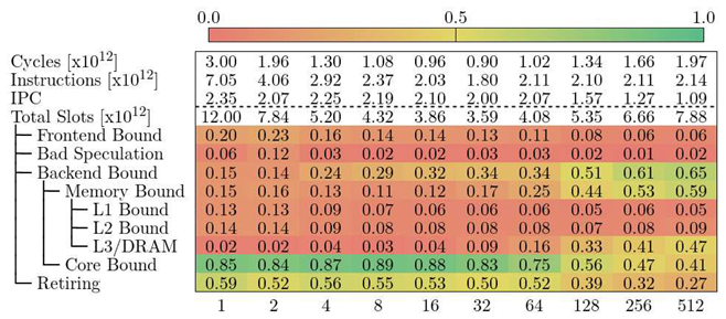
In this section we present the Top-Down model results for Alya in each system under study. We lay down the model hierarchy as tables. Rows represent metrics while each column represents runs with a given VECTOR_SIZE. The metrics above the dotted line are not part of the Top-Down model but provide complementary information that we consider relevant to analyze the metrics as a whole. Each cell contains the value of a given metric for a given run, and is color-coded with a gradient from red to (metric equals zero) to green (metric equals one). The reader should keep in mind that depending on the machine, the metrics represent a portion of the total amount of consumed slots (or cycles), while on others they represent a portion of the parent metric.

5.1. MareNostrum 4

Table 2 shows the Top-Down model for Alya in MareNostrum 4. We observe that the cycles decrease up to a VECTOR_SIZE of 32, after which they start to bounce back up. The number of executed instructions and the IPC also coincide with our previous knowledge of the application. The Top-Down model tells us that Alya in MareNostrum 4 is affected by different factors when increasing VECTOR_SIZE.

1 to 32 the majority of the cycles are categorized as Retiring, which means that the pipeline is not stalled. The reader should note the model does not provide insight on whether the instructions that go through the pipeline are useful calculations or not.

32-128 the code is Core Bound, which means that the pipeline is stalled due to the computational resources. The official definition of TMAM defines metrics under Core Bound, but the PAPI installation in MareNostrum 4 does not provide access to the necessary counters. An instruction mix or pipeline usage breakdown could give more information about which type of operation is clogging the CPU. Note however, that the Memory Bound metric is gradually increasing. This means that the pipeline stalls due to memory accesses are becoming more impactful.

128-512 the code falls under Memory Bound, which means that slots are lost because the pipeline is waiting for memory resources. Again, the original model describes detailed metrics that we cannot measure in MareNostrum 4. Furthermore, we do not know which actions could the programmer take in order to reduce memory pressure.

Since we were not able to construct further levels of the Top-Down model in MareNostrum 4, we cannot investigate further the Memory Bound category. However, we know from our previous study that the issue with high values of VECTOR_SIZE is related to the memory, so we can study the number of accesses and misses to the different levels of the memory hierarchy. In the Skylake CPU, the L2 cache is the last level of private cache. It is the highest level in the memory hierarchy where we can measure memory accesses per core. Figure 9 shows the evolution of L2 cache accesses (green bars, measured with PAPI_L2_TCA), L2 cache misses (purple bars, measured with PAPI_L2_TCM) and L2 miss ratio (line, measured as PAPI_L2_TCM/PAPI_L2_TCA).

We observe that the number of L2 cache accesses follows a U shape similar to the execution cycles. In contrast, the number of L2 cache misses stays flat from VECTOR_SIZE 1 to 32, and increases drastically for higher values. The combined view of L2 cache accesses and misses (miss ratio) shows that there is a noticeable jump starting at VECTOR_SIZE 32. This jump coincides with the point at which the elapsed time of Alya stops decreasing and the code modification appears to be detrimental. It also matches with the results presented in Table 2: the highest metric when VECTOR_SIZE is between 32 and 128 is Core Bound, but Memory Bound is the metric that is consistently increasing. We conclude that the code modification of Alya is beneficial in MareNostrum 4 up to VECTOR_SIZE 32, because it decreases the number of instructions executed and the number of L2 accesses. However, the modification reaches an inflexion point from which the L2 miss ratio becomes too high and the elapsed time bounces back up.

The Top-Down model has helped us to identify, in general terms, the part of the CPU that stalls during execution. However, more detailed metrics require access to hardware counters that are not accessible in our platform. This limits the insight that the model can provide. We can complement the information the Top-Down model gives us to compensate for the missing metrics (e.g., L2 accesses and misses). Without this complementary data, we cannot tell how execution cycles are lost. Furthermore, the study in MareNostrum 4 shows that only looking at the metric with the highest value does not tell the whole story.

5.2. CTE-AMD

Table 3 shows the Top-Down model for Alya in CTE-AMD. We observe a similar behavior as with MareNostrum 4 in Table 2 (i.e., the number of execution cycles decreases until VECTOR_SIZE 32, and bounces back up). In this case, we also identify the Backend Bound category to be the main limiting factor for high values of VECTOR_SIZE. However, the starting point of Backend Bound is 56% for CTE-AMD, while it is 13% for MareNostrum 4. Moreover, the portion of slots categorized as Retiring is always lower in CTE-AMD compared to MareNostrum 4. Unfortunately, we cannot drill further down because we have no definition of metrics nor more hardware counters available in the cluster.

5.3. CTE-Arm

Table 3 shows the Top-Down model for Alya in CTE-Arm. The top part represents the first three levels of the model while the bottom represents the metrics under Memory Bound. Like with MareNostrum 4 and CTE-AMD, the execution cycles decrease up to a certain value of VECTOR_SIZE and then they jump back up. We observe that in CTE-Arm, the values of VECTOR_SIZE 128 and 256 yield the lowest amount of cycles. This is a much higher VECTOR_SIZE compared to MareNostrum 4 and CTE-AMD, which were around 32 and 64.

Table 4. Top-Down model for Alya in CTE-Arm

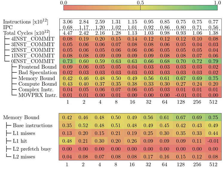The Top-Down model in CTE-Arm does not have a Retiring metric, like in MareNostrum 4. We can achieve a similar metric by combining {4,3,2,1}INST_COMMIT. This new metric groups cycles where at least one instruction was committed, which is similar to the definition of Retiring but includes cycles where the CPU could not commit some instruction. The key difference between the model in MareNostrum 4 in CTE-Arm that makes it impossible to have a comparable Retiring is that the first uses Slots to construct its metrics while the second uses Cycles.

Looking at the other end of the spectrum, we observe that for VECTOR_SIZE 1, CTE-Arm spends 75% of the execution cycles completely stalled (0INST_COMMIT). This trend is observable across all values of VECTOR_SIZE, with 4 showing the lowest (59%) value and 512 showing the highest (79%). The reader should note that the 0INST_COMMIT metric is indicative of how bad the pipeline is stalled, but it does not reflect the total execution time. Furthermore, the metric is relative to the total execution cycles, which means that the run with the lowest 0INST_COMMIT is not necessarily the fastest. As it stands, the Top-Down model in CTE-Arm does not allow us to compare metric-to-metric different runs. What it allows us to do, is to walk down the hierarchy in a particular run or observe general trends across runs.

For low values of VECTOR_SIZE, the metrics Memory Bound and Compute Bound are the main limiting factors. From VECTOR_SIZE 32 onward, Memory Bound accounts for more than half of the cycles lost in 0INST_COMMIT. We can further drill down and measure the metrics bellow Memory Bound (shown in the bottom part of Table 3). We observe that Base instructions is always the dominant metric, with the exception of VECTOR_SIZE 1 where L1 hit is higher. The description of this metric in the official documentation by Fujitsu [11] states: Cycles caused by instructions belonging to Base Instructions2. With only this definition, it is unclear if there is overlap between the metric and other metrics under Memory Bound, but Table 14-6 of the same document verifies that there is no overlap. Our observation is that there is an increase of the proportion of cycles lost due to L1 misses while the inverse happens for L1 hit. With the information available, we cannot blame the cycles lost waiting for the completion of a memory access Memory Bound to a specific type of load operation, we can only conclude that it is a scalar instruction (not SIMD nor SVE).

5.4. CTE-Power

Table 5 shows the Top-Down model for Alya in CTE-Power. Similar to CTE-Arm, the number of total cycles decreases while VECTOR_SIZE increases, but they start bouncing back up when VECTOR_SIZE is 512.

Throughout all the executions, the main limiting factor is the Pipeline stall category, which is comparable to the Retiring category in MareNostrum 4. Furthermore, the Memory subcategory represents always between 85% and 90% of the stalled cycles. In contrast, the Compute subcategory, the second highest, only accounts 15% max.

Drilling into the Memory category, we observe that there are two metrics which evolve noticeably when increasing VECTOR_SIZE: Store reorder queue and Store finish. While the first one represents 50% of the cycles due to memory stalls with VECTOR_SIZE 1, its weight decreases while the weight of Store finish increases.

Store reorder queue is defined by the counter PM_CMPLU_STALL_SRQ, which measures the cycles a store operation was stalled because the store-reorder-buffer (SRQ) was full (i.e., Too many store operations were in-flight at the same time).
Store finish is defined by the counter PM_CMPLU_STALL_STORE_FINISH, which measures the cycles waiting for a store operation that has all of its dependencies met to finish (i.e., The nominal latency of a store operation).

Following the definition of both metrics, we can infer that the parameter VECTOR_SIZE has an effect on the amount of store operations that are in-flight at the same time. For low values of the parameter (VECTOR_SIZE ≤ 16), there are too many stores at once, which stalls the pipeline. From that point forward, the concurrent store operations decrease, which means that the pipeline is still waiting for stores to complete, but these have a minimum amount of cycles to complete (pipeline latency). The Top-Down model in CTE-Power is heavily dependent on the micro-architecture, so going deep into the hierarchy might give more insight about performance bottlenecks, but makes it harder to compare against other machines.

5.5. CTE-Kunpeng

Table 6 shows the Top-Down model for Alya in CTE-Kunpeng. Furthermore, the model has been defined to be very similar to the original Top-Down model from Intel. Contrary to MareNostrum 4, the results in CTE-Kunpeng show that Core Bound is the main limiting factor for low values of VECTOR_SIZE. We know that the CPU in CTE-Kunpeng has a lower single-thread performance compared to MareNostrum 4 (see Table 1). In the case of Alya, the weaker floating-point throughput of the core is reflected as cycles stalled due to the computational resources being occupied. At the time of writing, we do not have the definition of the metrics under Core Bound, so we cannot construct the whole hierarchy.

As VECTOR_SIZE increases, so does the Memory Bound metric. Starting at VECTOR_SIZE 256, Alya has become bounded by the memory subsystem. For the Memory Bound part, we can study the different cache levels in CTE-Kunpeng. This in-depth study was not possible in MareNostrum 4 since we lacked the PAPI counters to compute the metrics. At this point, the model suggest that cycles are being lost due to L3 Cache and DRAM accesses or misses. The cache hierarchy of the Kunpeng 920 CPU shares the L3 level across cores, which makes it difficult to blame accesses or misses to a particular core.

6. Conclusions

In this paper, we have studied the Top-Down model for three different ISAs (x86-64, Arm-v8 and IBM Power9) implemented by five different chip providers (Intel, AMD, Fujitsu, Huawei and IBM) in five HPC clusters. We used Alya, a CFD application, as a vehicle to measure the metrics of each model and gain insights about performance bottlenecks. The results of our study can be summarized into two main categories: i) conclusions that can be drawn when studying the top-down model within the same cluster and ii) considerations that relate to the top-down results gathered from different clusters.

Within the same cluster we found that the implementation of the Top-Down model can be tricky: going deep into the hierarchy of the model means needing hardware counters, which are not always available due to limitation in tools maturity or system software configuration. Also, some architectural details can be missing.

On a case-by-case, x86-64 Skylake is the most documented and with official support by Intel. The metrics are well defined and easy to understand, but they require hardware counters that are not available in MareNostrum 4. This issue is even more apparent in CTE-AMD, where we were not able to go past the first level of metrics of the Top-Down model. In the case of CTE-Power, the amount of counters needed to construct the whole hierarchy implies obtaining the data with multiple runs. Once constructed, interpreting the metrics requires a deeper understanding of the micro-architecture of the system compared to the other clusters. The model in CTE-Arm tries to strike a balance: the official documentation accompanies the Cycle Accounting with multiple tables of complementary metrics so we were able to go beyond the first level of metrics. However, the model definition in CTE-Arm does not allow for metric comparisons between runs because metrics are relative to their parent in the tree and not to the root.

Once mapped the hardware counters on the Top-Down model in a given system, we comment about the insights we can obtain from the model itself. The metrics are always defined relative to the execution cycles (or parent metric) of their respective runs. Thus, when comparing runs performed with different software configurations (e.g., changing VECTOR_SIZE) on the same cluster, having a higher or lower value of a certain metric does not imply a better or worse execution time. The Top-Down model only shows general trends and how this evolves throughout different runs with different configurations (e.g., changing VECTOR_SIZE). Once constructed, the interpretation of the metrics in all clusters depends on micro-architectural knowledge.

Among different clusters we discover even more limitations. Having no common naming-convention of metrics across systems, makes it hard to compare the results of Top-Down models gathered on different clusters. Even with the same names, metrics in different systems have subtle differences: e.g., on MareNostrum 4, CTE-AMD, and CTE-Kunpeng the inefficiencies of the Top-Down model are gathered on the boundary between front-end and back-end of the CPU, while on CTE-Arm and CTE-Power the model counts the cycles lost during the commit stage of the instructions.

We have seen that on different machines we can go deeper in the hierarchy of the model, depending on availability of hardware counters. However, even having access to the whole Performance Monitoring Unit (where hardware counters are stored) does not magically mean having more insight because a correct interpretation of the most of the counters requires a deep knowledge of the underlying micro-architecture that the scientist running a scientific code does not have. This creates a trade-off when using the Top-Down model: The deeper the detail and insight, the more it depends on previous micro-architecture knowledge and the more difficult it becomes to compare against other machines. Moreover, in some clusters the definition of the model requires architectural parameters which makes more difficult the work of defining the model and comparing with other clusters.

As general and most important remark, we conclude that there is no metric in none of the models that tell how much the CPU resources are being used. One could measure

100 %

of Slots in the Retiring category, but that does not tell if the code is running efficiently: it simply tells that there are no pipeline stalls. In the Top-Down model defined by Intel, there are some metrics under the Retiring category which try to tell if there is room for improvement. However, we did not include these metrics in our work because (once more) we were limited by the available hardware counters.

While the Top-Down model is accepted by the community as a method for spotting inefficiencies of HPC codes, we have experienced that:

it requires additional information (either micro-architectural details or further hardware counters) to draw a full picture when analyzing and improving the performance of a scientific application;
it does not quantify how much each of the resources within the compute node are used/saturated;
it does not allow to easily compare among clusters of the same architecture, nor different architectures.

All these limitations makes the work very difficult to a performance analyst that wants to use the Top-Down model as an inspection tool for spotting inefficiencies in complex scientific codes. The dependencies with the micro-architectural knowledge makes it also not feasible to be proposed as co-design tool to the researcher owner of the scientific application under study.

Author Contributions

All authors have contributed equally to the work reported.

Funding

This research received no external funding.

Institutional Review Board Statement

Not applicable.

Data Availability Statement

The data presented in this study are available on request from the corresponding author.

Acknowledgments

The authors thank the support team of Dibona operating at ATOS/Bull. This work is partially supported by the Spanish Government through Programa Severo Ochoa (SEV-2015-0493), the Spanish Ministry of Science and Technology project (TIN2015-65316-P), the Generalitat de Catalunya (2017-SGR-1414), the European Community’s Seventh Framework Programme [FP7/2007-2013] and Horizon 2020 under the Mont-Blanc projects (grant agreements n. 288777, 610402 and 671697), the European POP2 Center of Excellence (grant agreement n. 824080), and the Human Brain Project SGA2 (grant agreement n. 785907).

Conflicts of Interest

The authors declare no conflict of interest.

Appendix A. Event sets and metrics

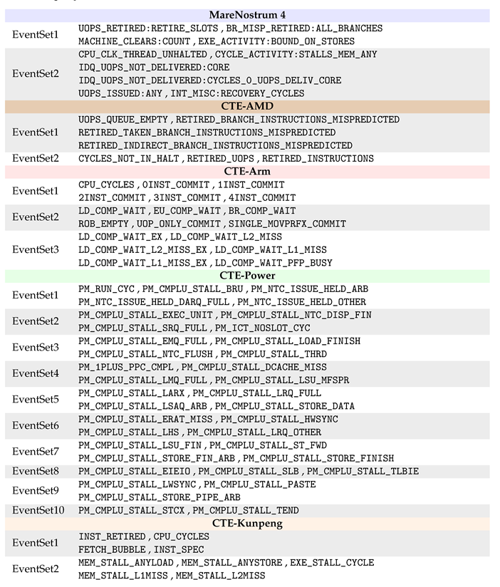
In Table A1, we list the PAPI Event sets used to construct the Top-Down model on each system under study. The left column displays the name of the event set, while the right column lists the PAPI events included in a given set. Events repeated in more that one set are omitted.

Table A1. Event set reference for MareNostrum 4, CTE-AMD, CTE-Arm, CTE-Power, and CTE-Kunpeng

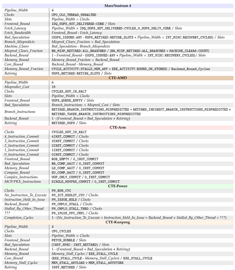
In Table A2, we list the PAPI counters and formulas used to construct the Top-Down model on each system under study. The left column displays the name of a metric, while the right column details the formula to compute the metric. Counters are written in monospace font and using the exact same name as displayed by the papi_native_avail command. Metrics of the model as well as helper metrics are written in cursive.

Table A2. Top-Down model counter reference for MareNostrum 4, CTE-AMD, CTE-Arm, CTE-Power, and CTE-Kunpeng

References

Top500 list, 2022.
Williams, S.; Waterman, A.; Patterson, D. Roofline: An Insightful Visual Performance Model for Multicore Architectures. Commun. ACM 2009, 52, 65–76. [Google Scholar] [CrossRef]
Ofenbeck, G.; Steinmann, R.; Caparros, V.; Spampinato, D.G.; Püschel, M. Applying the roofline model. 2014 IEEE International Symposium on Performance Analysis of Systems and Software (ISPASS). IEEE, 2014, pp. 76–85.
Ilic, A.; Pratas, F.; Sousa, L. Cache-aware Roofline model: Upgrading the loft. IEEE Computer Architecture Letters 2014, 13, 21–24. [Google Scholar] [CrossRef]
Banchelli, F.; Garcia-Gasulla, M.; Houzeaux, G.; Mantovani, F. Benchmarking of State-of-the-Art HPC Clusters with a Production CFD Code. Proceedings of the Platform for Advanced Scientific Computing Conference; Association for Computing Machinery: New York, NY, USA, 2020. [Google Scholar] [CrossRef]
Yasin, A. A Top-Down method for performance analysis and counters architecture. 2014 IEEE International Symposium on Performance Analysis of Systems and Software (ISPASS), 2014, pp. 35–44. [CrossRef]
Intel. Top-down Microarchitecture Analysis Method, 2022.
Jarus, M.; Oleksiak, A. Top-Down Characterization Approximation based on performance counters architecture for AMD processors. Simulation Modelling Practice and Theory 2016, 68, 146–162. [Google Scholar] [CrossRef]
Banchelli, F.; Oyarzun, G.; Garcia-Gasulla, M.; Mantovani, F.; Both, A.; Houzeaux, G.; Mira, D. A portable coding strategy to exploit vectorization on combustion simulations, 2022, [arXiv:cs.DC/2210.11917].
Fog., A. The microarchitecture of Intel, AMD, and VIA CPUs - An optimization guide for assembly programmers and compiler makers, 2022.
A64FX Microarchitecture Manual, 2021.
POWER9 Performance Monitor Unit User’s Guide, 2018.
Unified European Applications Benchmark Suite. http://www.prace-ri.eu/ueabs/ - Last accessed Nov. 2016.
Terpstra, D.; Jagode, H.; You, H.; Dongarra, J. Collecting Performance Data with PAPI-C. Tools for High Performance Computing 2009; Müller, M.S.; Resch, M.M.; Schulz, A.; Nagel, W.E., Eds.; Springer Berlin Heidelberg: Berlin, Heidelberg, 2010; pp. 157–173.
Pillet, V.; Pillet, V.; Labarta, J.; Cortes, T.; Cortes, T.; Girona, S.; Girona, S.; Computadors, D.D.D. PARAVER: A Tool to Visualize and Analyze Parallel Code. Technical report, In WoTUG-18, 1995.

1	Except for memory metrics
2	The set of Base Instructions in the Armv8 ISA contains basic scalar arithmetic and memory instructions.

Figure 1. Top-Down model hierarchy in MareNostrum 4

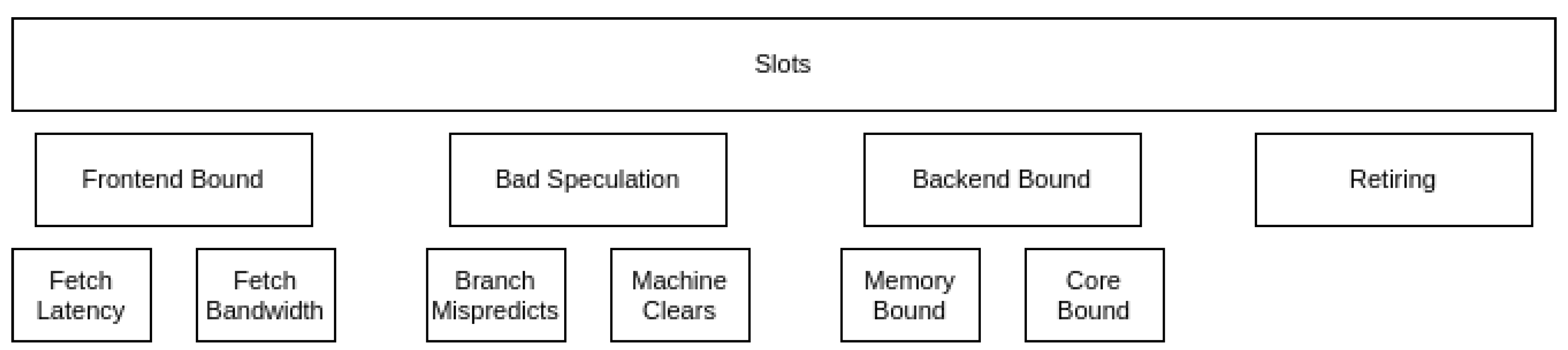
Figure 2. Top-Down model hierarchy in CTE-AMD

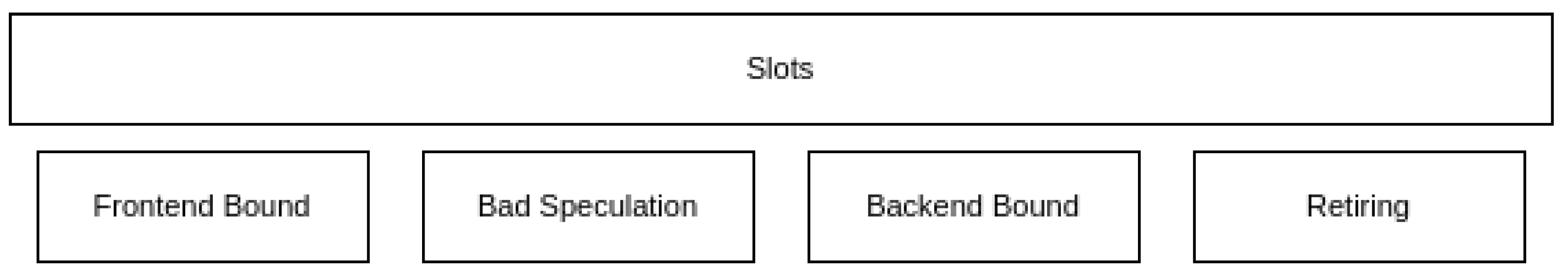
Figure 3. Top-Down model hierarchy in CTE-Arm

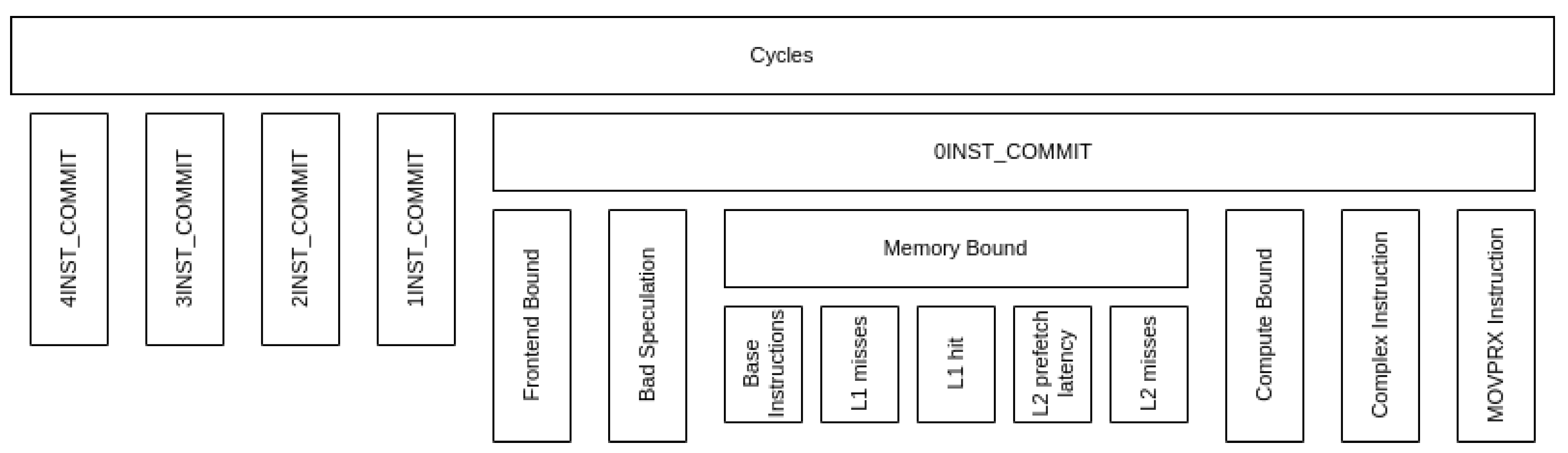
Figure 4. Top-Down model hierarchy in CTE-Power

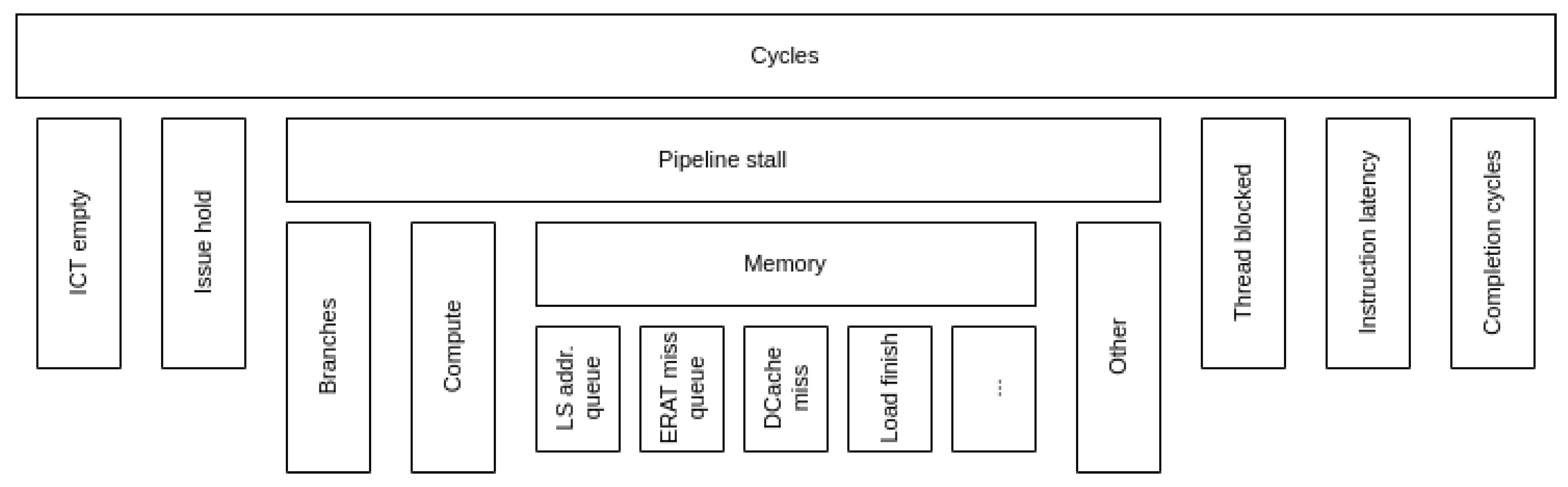
Figure 5. Top-Down model hierarchy in CTE-Kunpeng

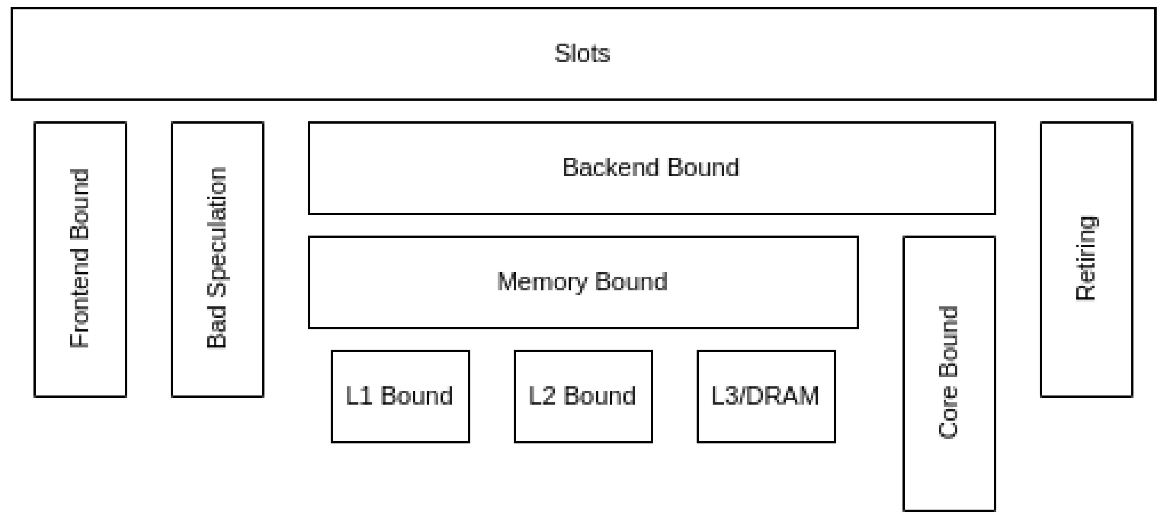
Figure 6. Timeline of one timestep in Alya

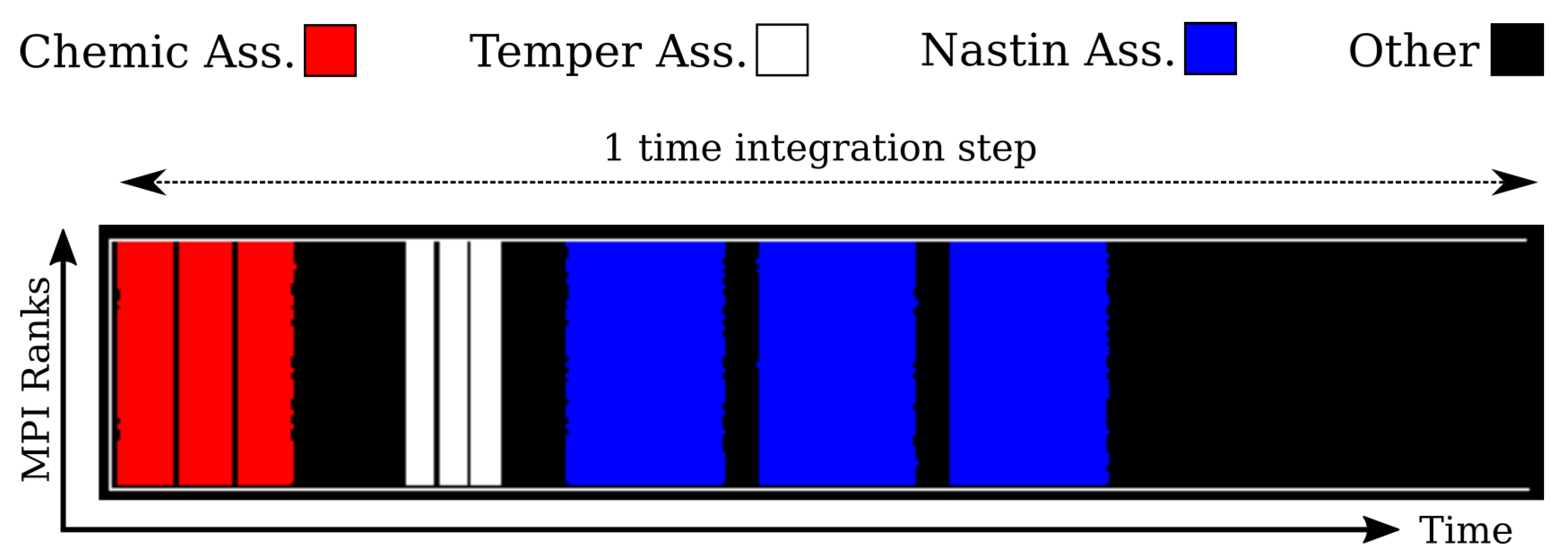
Figure 7. Paraver timeline examples. Top: quantitative representation of number of instructions. Bottom: MPI primitive calls.

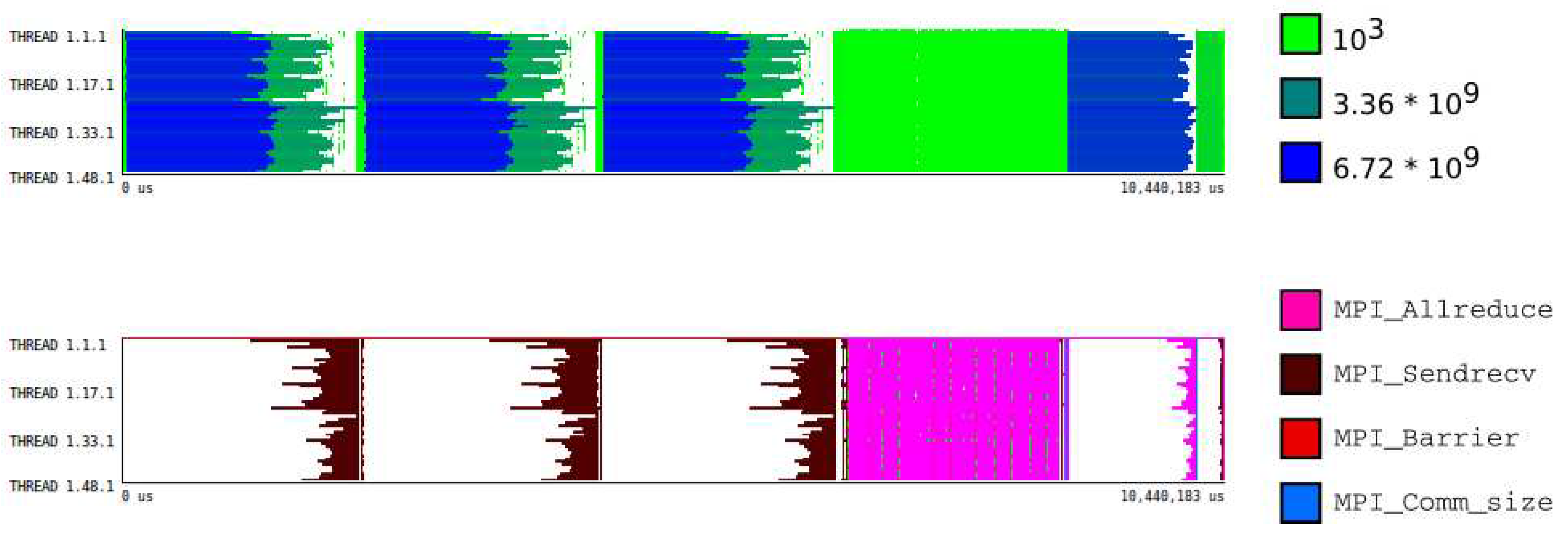
Figure 8. Workflow from application execution to model results

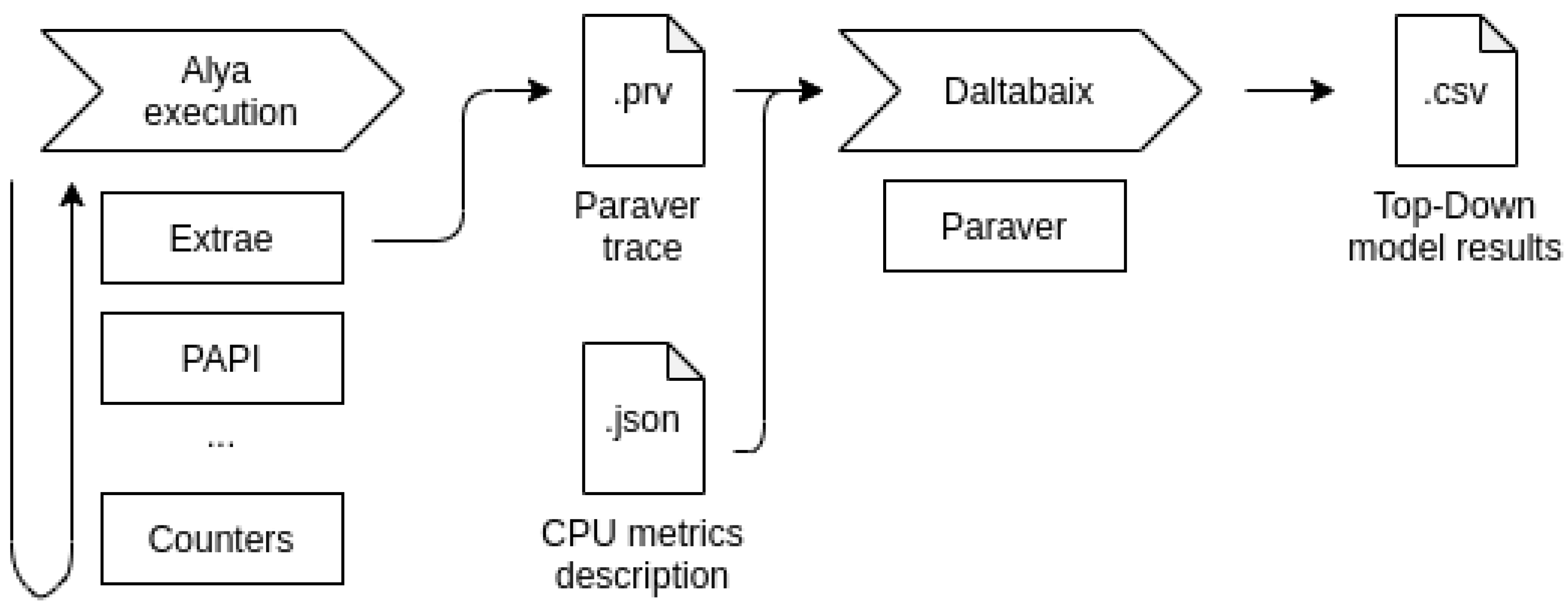
Figure 9. L2 accesses and misses in MareNostrum 4

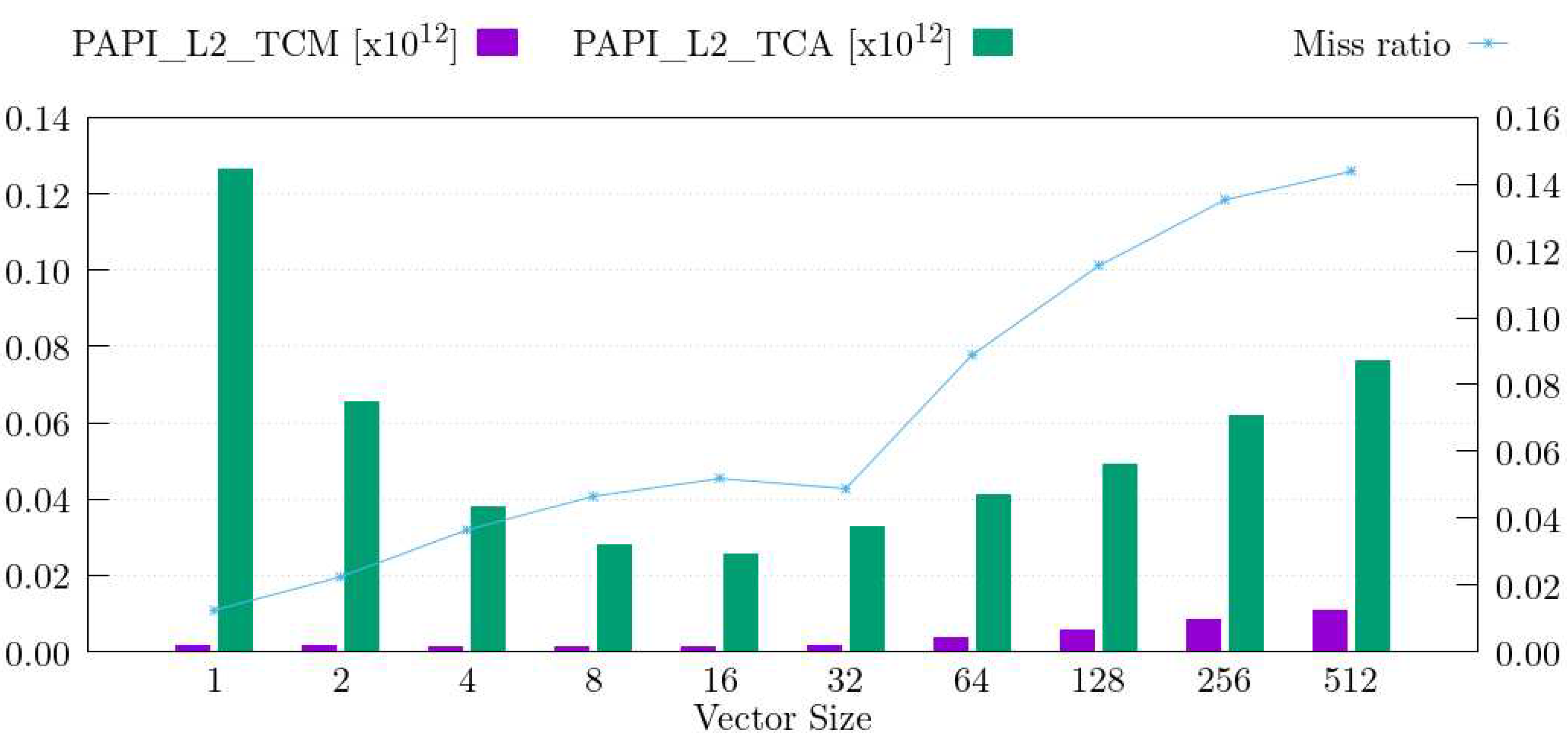
Table 1. Hardware and software configurations for MareNostrum 4, CTE-AMD, CTE-Arm, CTE-Power, and CTE-Kunpeng

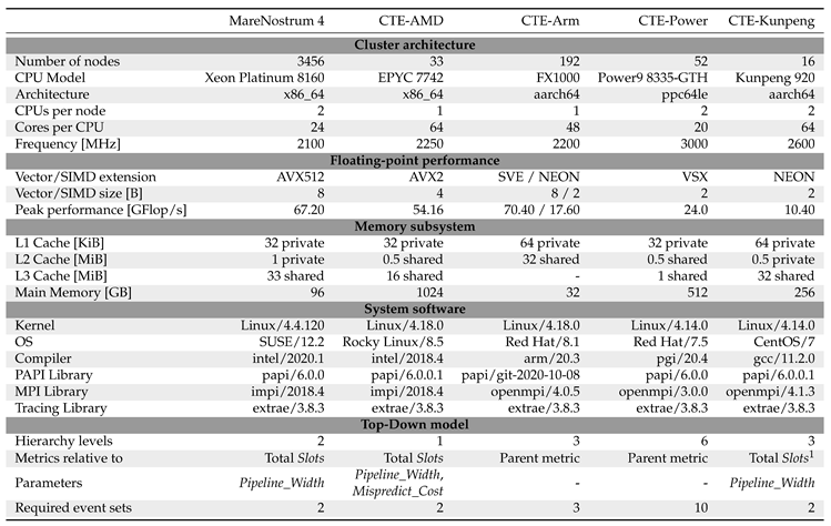Table 2. Top-Down model for Alya in MareNostrum 4

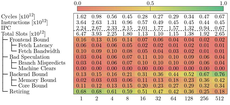Table 3. Top-Down model for Alya in CTE-AMD

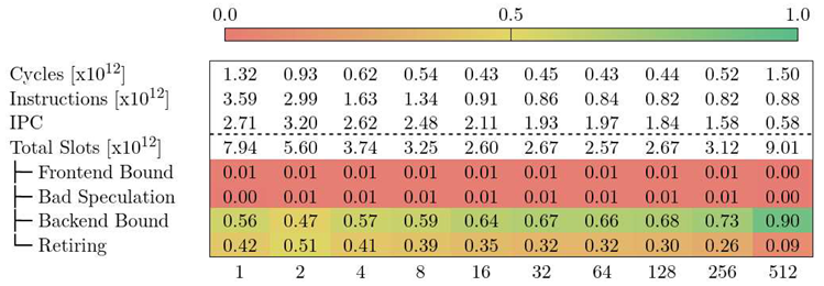Table 5. Top-Down model for Alya in CTE-Power

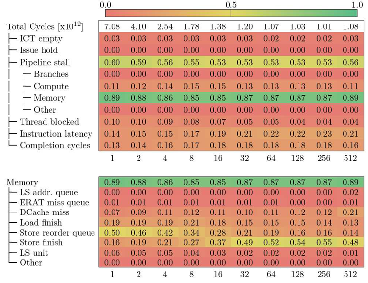Table 6. Top-Down model for Alya in CTE-Kunpeng

Disclaimer/Publisher’s Note: The statements, opinions and data contained in all publications are solely those of the individual author(s) and contributor(s) and not of MDPI and/or the editor(s). MDPI and/or the editor(s) disclaim responsibility for any injury to people or property resulting from any ideas, methods, instructions or products referred to in the content.

© 2023 by the authors. Licensee MDPI, Basel, Switzerland. This article is an open access article distributed under the terms and conditions of the Creative Commons Attribution (CC BY) license (http://creativecommons.org/licenses/by/4.0/).

Copyright: This open access article is published under a Creative Commons CC BY 4.0 license, which permit the free download, distribution, and reuse, provided that the author and preprint are cited in any reuse.

Downloads

289

Views

Comments

Subscription

Notify me about updates to this article or when a peer-reviewed version is published.

MDPI Initiatives

Important Links

Choose an area of interest and we will send you notifications of new preprints at your preferred frequency.

Disclaimer