Graph Neural Networks (GNN) for Tensile Strength Prediction in Additive Manufacturing

Preprint

Article

Graph Neural Networks (GNN) for Tensile Strength Prediction in Additive Manufacturing

Altmetrics

Downloads

216

Views

101

Comments

Akshansh Mishra^*

Vijaykumar S. Jatti^*

Akshansh Mishra^*

Vijaykumar S. Jatti^*

This version is not peer-reviewed

Submitted:

13 August 2023

Posted:

14 August 2023

You are already at the latest version

Alerts

Abstract

This paper presents the use of Graph Neural Networks (GNNs) to predict the tensile strength of Fused Deposition Modeling (FDM) specimens. In the present work, there are four main input parameters i.e. Infill percentage, Layer height, Print speed and Extrusion temperature while the Tensile Strength is an output parameter were considered. This study includes use of central composite design based response surface methodology to finalize the experimental layout. 3D printed specimen were manufactured as per the ASTM E8 standard on FDM printer using Polylactic Acid (PLA) as filament. Micro-tensile test were performed on the printed specimen as per ASTM E8 standard. The GNN algorithm was trained on a dataset of FDM specimens, achieving a mean squared error (MSE) of 2.47, mean absolute error (MAE) of 1.14, and R-squared value of 0.78. An adjacency matrix, which shows the connections between nodes in a graph. The obtained plot for nodes and weights in a GNN provide valuable information about the model and its performance. The results show the potential of using GNNs in predicting the mechanical properties of additively manufactured specimens and provide a promising direction for further research in this field.

Keywords:

Subject: Engineering - Mechanical Engineering

1. Introduction

Graph Neural Networks (GNNs) represent a category of advanced machine learning algorithms that specifically handle data organized in graph structures. Unlike conventional neural networks, which are tailored for grid-based data like images or tables, GNNs are designed to effectively process data structured as graphs. In these graphs, nodes symbolize distinct entities, while edges signify relationships connecting these entities [1,2,3,4,5].

GNNs operate by accumulating information from neighboring nodes within a graph and leveraging this information to make informed predictions about node properties. This process hinges on the application of graph convolutional layers, which apply learned filters to the graph layout, thereby gathering insights from neighboring nodes and refining the representation of each node. GNNs have proven versatile across numerous applications, including recommendations, protein structure prediction, and social network analysis. Their strength lies in tackling scenarios where intricate entity relationships are prevalent, as they excel at capturing the intricate interplay of relationships within graph-based data [6,7,8,9].

Hestroffer et al. [10] pioneered the concept of Graph Neural Networks (GNNs) to accurately predict the mechanical attributes of polycrystalline materials. They devised a GNN model that employed a graph representation of polycrystals, encompassing essential grain characteristics such as size, crystal orientation, and neighboring grain connections. In the realm of additive manufacturing research, Graph Neural Networks (GNNs) carry the potential to revolutionize the field. Additive manufacturing involves the layer-by-layer construction of physical objects, often leading to end products with diverse mechanical traits, like tensile strength. Mozaffar et al. [11] introduced a graph-based model with neural networks to capture the intricate spatiotemporal relationships within additive manufacturing processes, focusing on the Directed Energy Deposition technique. The outcomes demonstrated that this deep learning framework adeptly forecasts thermal histories for unfamiliar geometries during training, offering a viable alternative to resource-intensive computational methods.

GNNs hold promise for modeling and predicting the mechanical characteristics of additively manufactured samples which find application in aerospace and biomedical sector as well [12,13,14,15], as they decipher the intricate connections between different geometric attributes and the corresponding mechanical traits. This approach unveils valuable insights into the nexus between specimen geometry and mechanical behavior, thereby guiding the optimization of the manufacturing procedure. Notably, this study introduces a pioneering application of the Graph Neural Network (GNN) model for predicting the properties of additively manufactured specimens.

2. Problem Statement

In this study, we investigate the use of Graph Neural Networks (GNNs) to forecast the tensile strength of specimens produced using Fused Deposition Modeling (FDM). Infill %, Layer height, Print speed, and Extrusion temperature are the four main input parameters used in the inquiry, with the goal of estimating the Tensile Strength as the output parameter. To optimize the experimental design, the study combines response surface approach and central composite design.

Polylactic Acid (PLA) filament is used to 3D print specimens that adhere to ASTM E8 requirements on an FDM printer in order to undertake the experimental analysis. The fabricated specimens are subjected to ASTM E8-recommended micro-tensile tests. We train a dataset of FDM specimens using the Graph Neural Network (GNN) technique.

The study also explores how to build an adjacency matrix, which reveals how nodes in a graph are connected to one another. The nodes and weights within the GNN are seen as a result, and this provides important insights into the properties and effectiveness of the model. The results illustrate the potential of GNNs in predicting the mechanical characteristics of specimens made using additive manufacturing, outlining a promising path for furthering study in this area.

3. Experimental Procedure

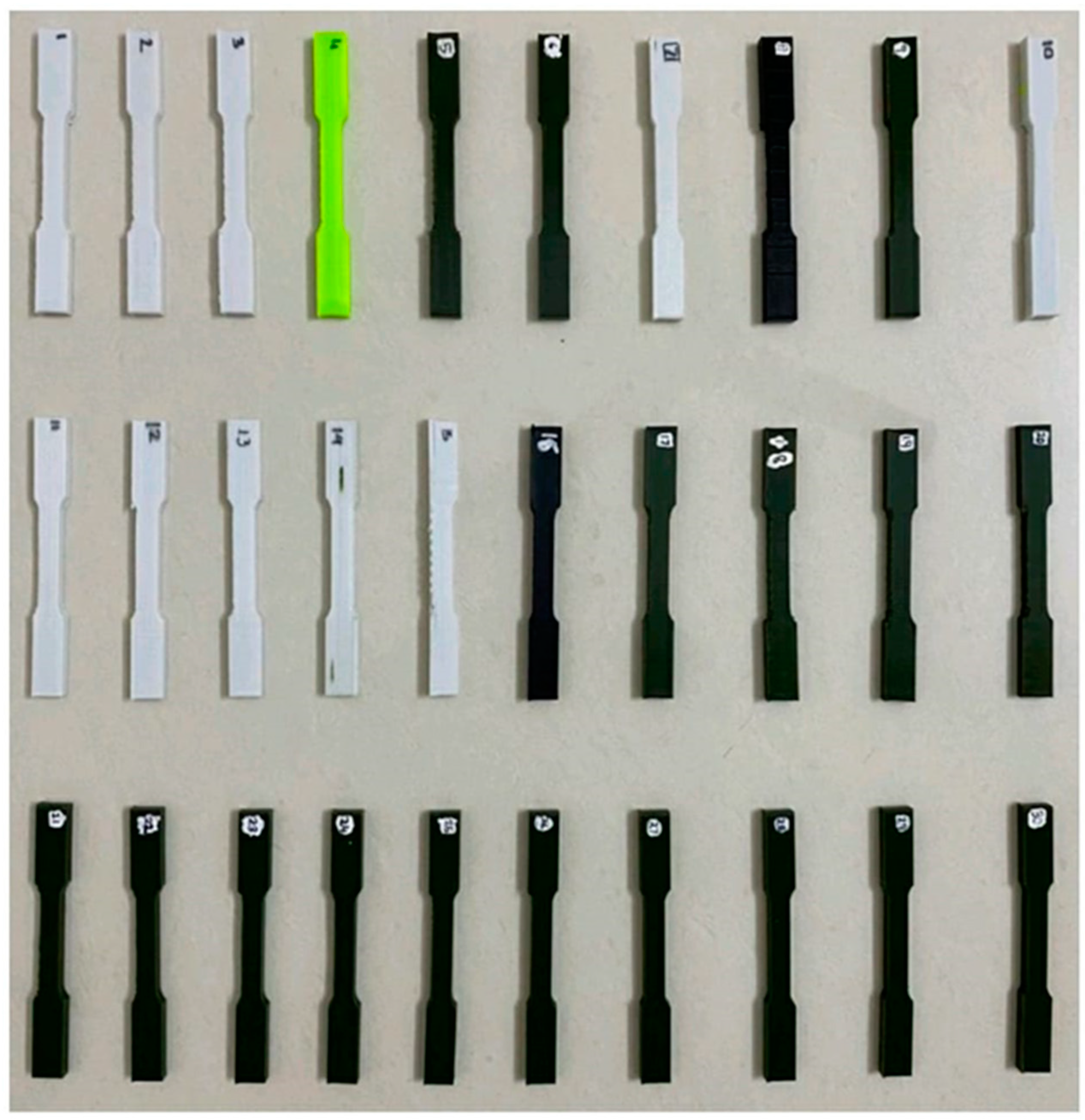
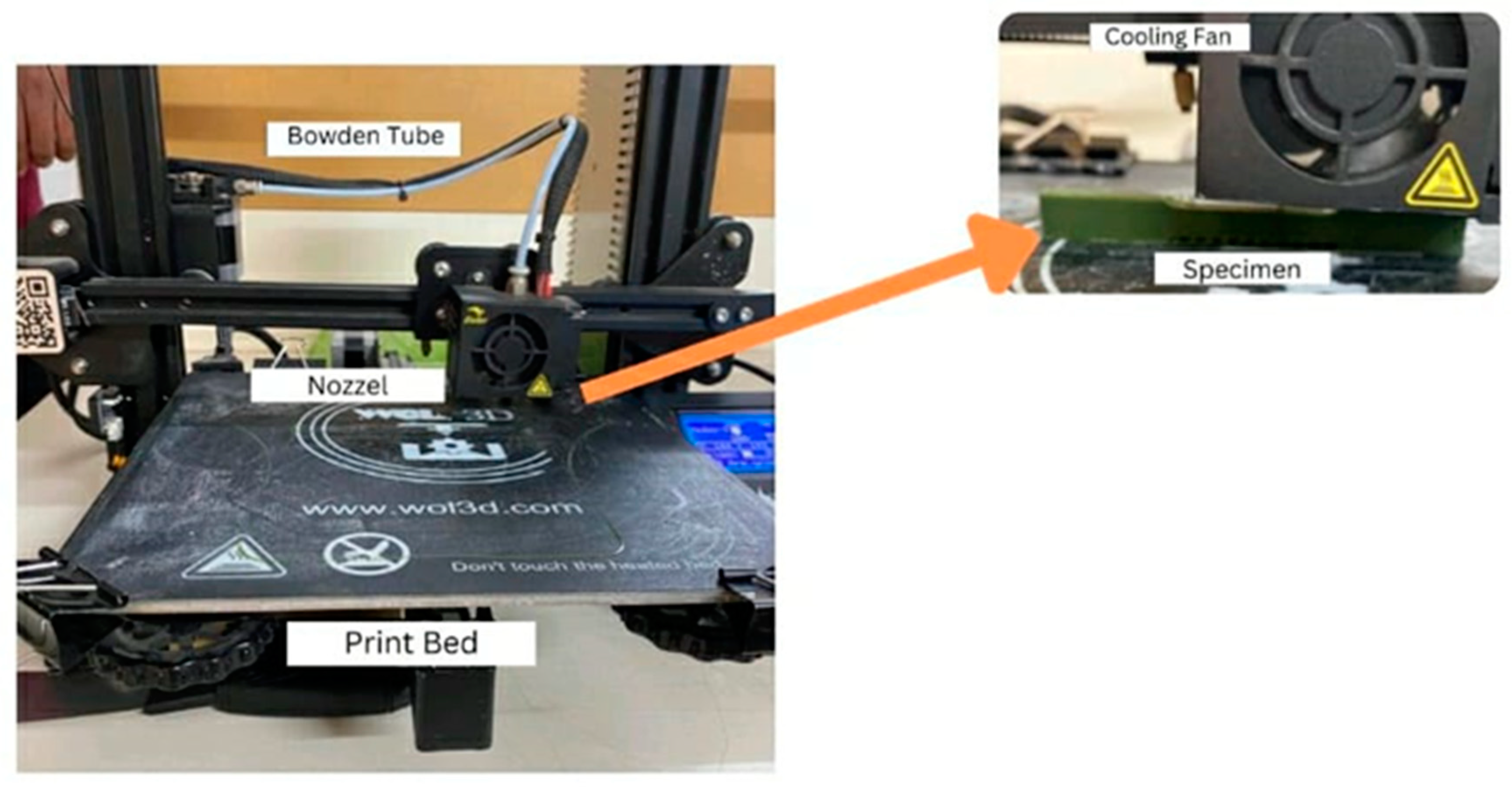
To establish a standardized framework, the ASTM E8 standard geometry was selected as the reference, and its dimensions were uniformly reduced by 50% to optimize printing size and material consumption, while minimizing production time. The Response Surface Methodology (RSM) Design of Experiment approach was utilized to formulate a series of 30 distinct trial conditions, illustrated in Figure 1, encompassing three levels for each input parameter. Subsequently, the CAD model was sliced accordingly and translated into G-code via Ultimaker Cura software. The empirical exploration was conducted utilizing a Creality 3D FDM printer, as depicted in Figure 2. Each printing session was assigned a unique configuration of settings, varying parameters such as layer height, infill density, infill pattern, bed temperature, and nozzle temperature, all tailored to produce Polylactic Acid (PLA) specimens. A comprehensive datasheet was generated to systematically organize these input parameters.

The FDM samples used in this research were fabricated with a Creality Ender 3 printer, which boasts a build area of 220 × 220 × 250 mm³. The measurements of the tensile specimen adhere to the specifications outlined in ASTM D638, with dimensions of 63.5 × 9.53 × 3.2 mm, meeting the prescribed criteria. Table 1 shows the experimental results obtained corresponding to the given input parameters.

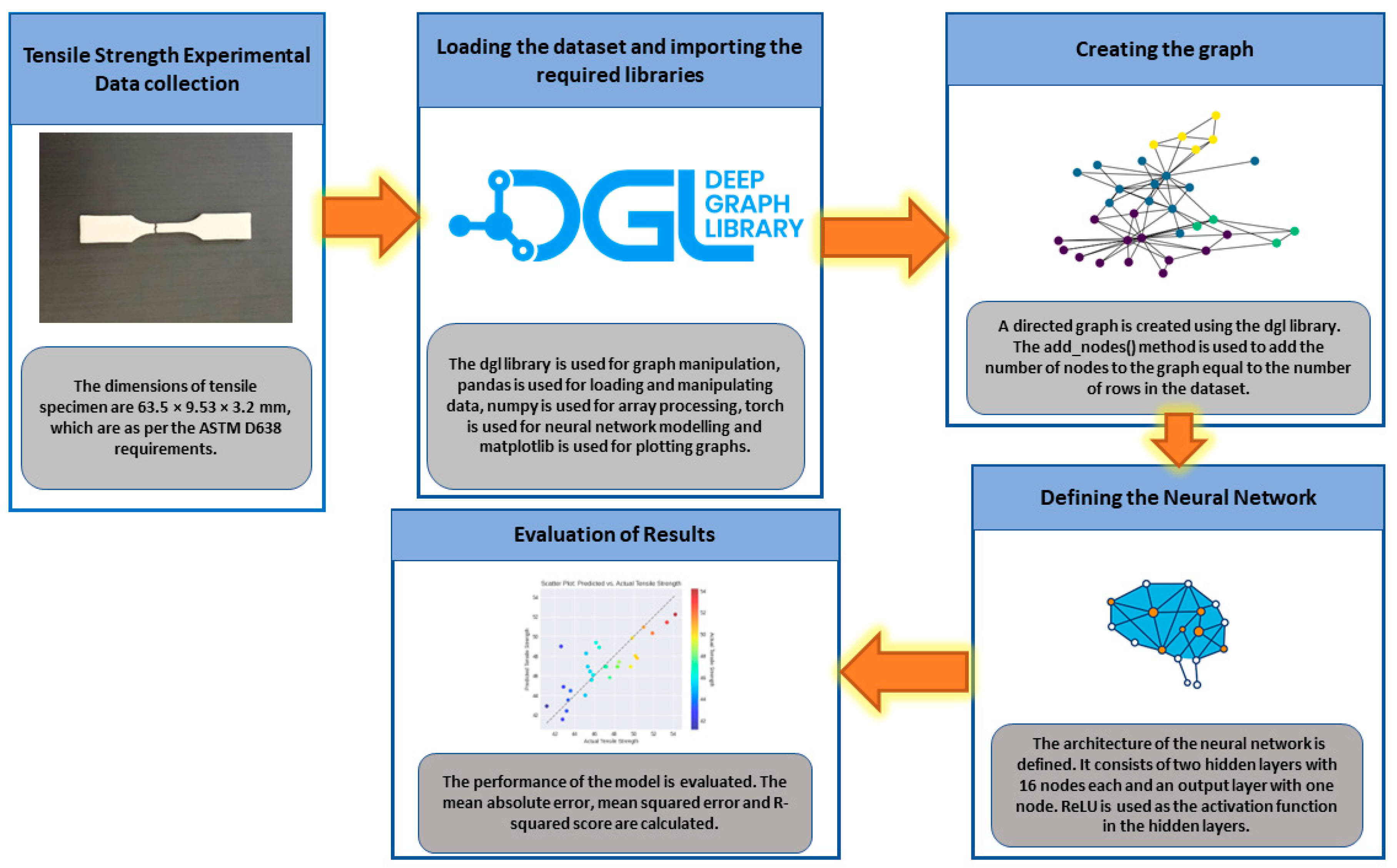
Figure 3 shows the implemented framework in the present study. All the necessary libraries required to build and train a graph neural network were imported.

The dgl library is used for graph manipulation, pandas is used for loading and manipulating data, numpy is used for array processing, torch is used for neural network modelling and matplotlib is used for plotting graphs. The dataset is imported from the CSV file and stored it in a pandas data frame. A directed graph is created using the dgl library. The add_nodes() method is used to add the number of nodes to the graph equal to the number of rows in the dataset. The performance of the model is evaluated by calculating the mean absolute error, mean squared error and R-squared score.

4. Results and Discussion

A Graph Neural Network (GNN) uses graph-structured data to train node representations that include both node-level properties and the underlying graph structure. The GNN functions in a message-passing framework, where information is transmitted between nodes through edges, given a graph with nodes (representing instances) and edges (representing links or connections). Message aggregation and updating node representations are the two fundamental processes of the mathematical formulation. The dataset's columns correspond to various features, and each row represents a node. The input columns for the node features (X) are "Infill percentage," "Layer height," "Print speed," and "Extrusion temperature".

Let

X

be the matrix of the node features where each row

x_{i}

corresponds to the feature vector of node

i

. The adjacency matrix

(A)

encodes the connections between nodes. Now, let

A

be the adjacency matrix of the graph where

A_{i j} = 1

if there is an edge between the nodes

i

and

j

and

A_{i j} = 0

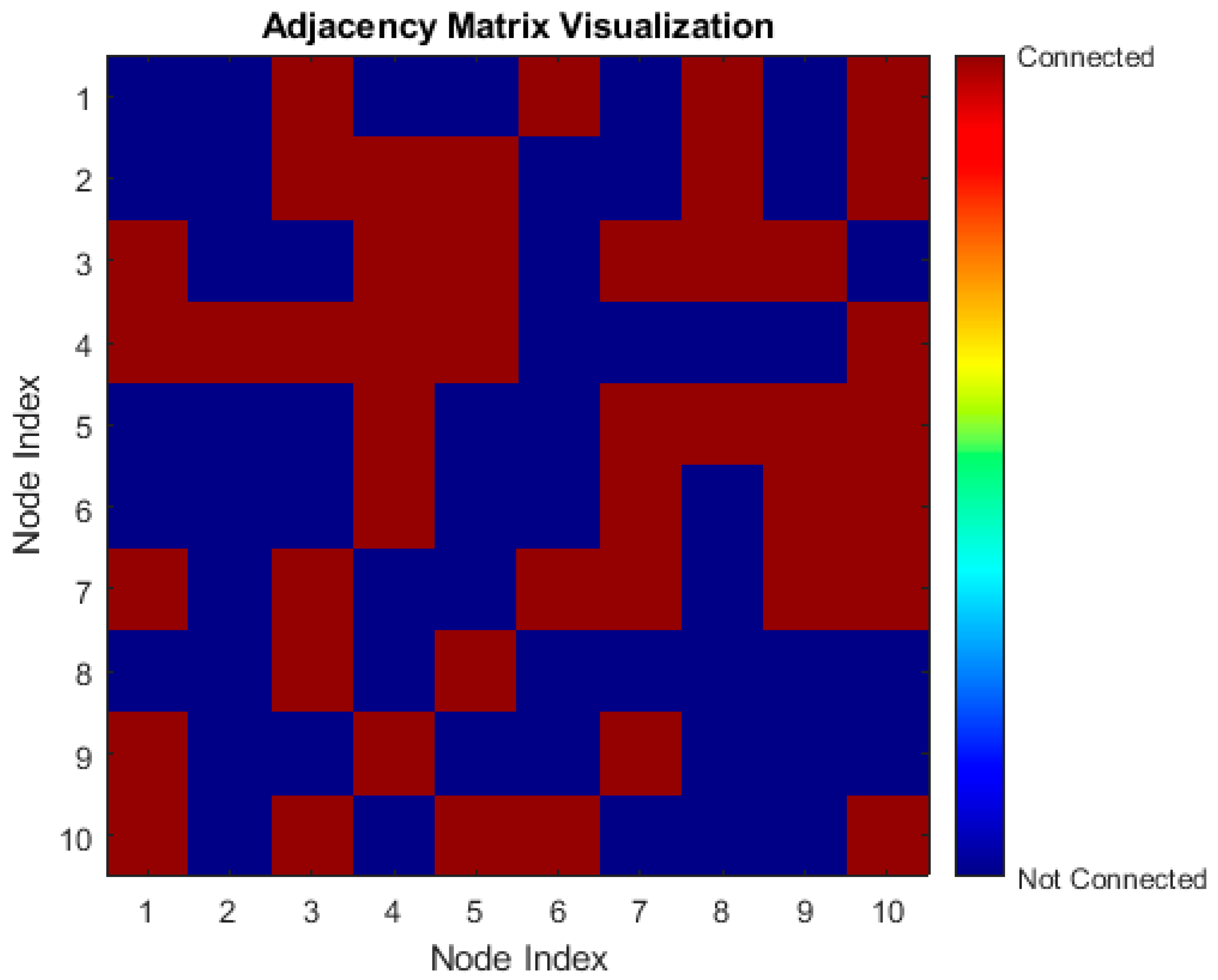
in the opposite condition as shown in Figure 4. We adopted a technique that is frequently used to express the connections between nodes to produce the adjacency matrix (A) for our graph-based study. Src_nodes and dst_nodes are two arrays that we defined in this procedure. These arrays stand in for the source and destination nodes of the edges in our graph, respectively. The corresponding entry in the dst_nodes array identifies the destination node of the same edge, while each entry in the src_nodes array identifies the originating node of an edge. We created the edges of the network by methodically creating links between the nodes by pairing these arrays.

In the message aggregation process, messages from nearby nodes are computed and aggregated to create a combined message for each node. In the graph, this gathers data from the node's neighbors. A learnable function is often used to define the aggregation process as shown in Equation 1.

M e s s a g e s^{(l + 1)} = σ (\sum_{j ϵ n e i g h b o u r s (i)} W^{(l)} . x_{j}^{(l)})

(1)

Where

l

is the layer index,

x_{j}^{(l)}

is the feature vector of node

j

in layer

l

n e i g h b o u r s (i)

represents the neighbors of node

i

W^{(l)}

is a learnable weight matrix for layer

l

,and

σ

is a non-linear activation function.

The node representations are updated using the aggregated messages and the node's own features after message aggregation. This stage captures the impact of both the graph structure and local node attributes as shown in Equation 2.

x_{i}^{(l + 1)} = M e s s a g e A g g r e g a t i o n^{(l + 1)} . (x_{i}^{(l)}, M e s s a g e s^{(l + 1)})

(2)

Predictions are made using the node representations after they have been obtained. In this instance, tensile strength values are predicted using regression using the GNN. For regression problems, the mean squared error (MSE) loss function is frequently employed as shown in Equation 3.

L o s s = \frac{1}{N} \sum_{i = 1}^{N} {(y_{i} - {\hat{y}}_{i})}^{2}

(3)

Where

N

is the number of instances (nodes) in the dataset,

y_{i}

is the true label (ground truth) for node

i

, and

{\hat{y}}_{i}

is the predicted label (output of the GNN) for node

i

The GNN parameters (weight matrices in this case) are updated to minimize the loss using an optimization algorithm such as Adam as shown in Equation 4.

θ^{(l + 1)} = θ^{(l)} - α . \nabla L o s s

(4)

Where

θ^{(l)}

is the parameter set (weights) of layer

l

α

is the learning rate, and

\nabla L o s s

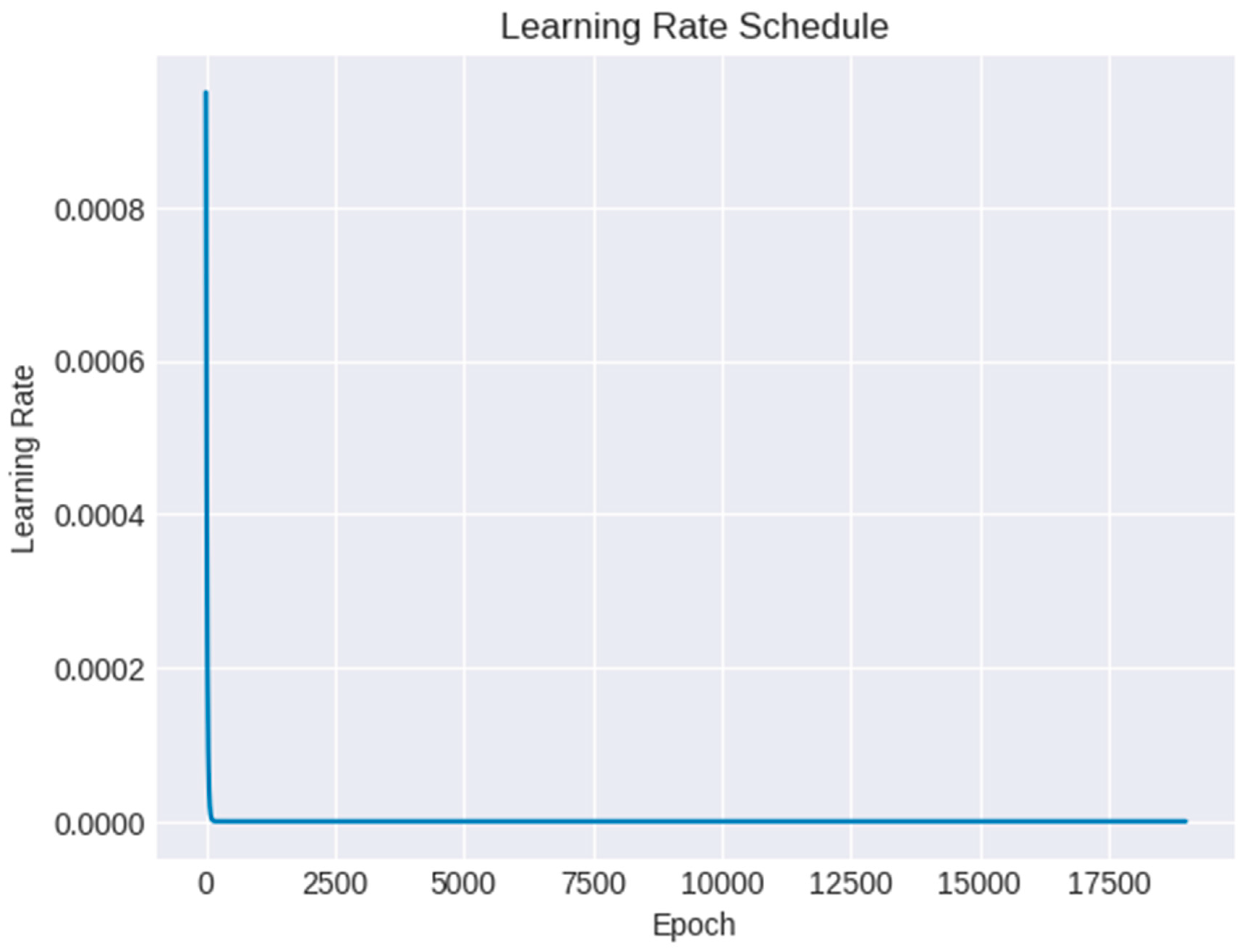
is the gradient of the loss with respect to the parameters. Figure 5 shows the plot of learning rate with increasing number of epochs. Especially during the optimization process, the plot of learning rate with increasing number of epochs is a useful visualization that offers insights into the training dynamics and convergence behavior of a machine learning model. The use of a learning rate schedule, where the learning rate changes over time (for example, progressively declines), is advantageous for some models. The plot can demonstrate the success or failure of the learning rate schedule in achieving a smooth and constant convergence trajectory. The plot also demonstrates the speed at which the optimization process reaches a minimum. The parameter updates could oscillate and stop converging at an excessive learning rate. However, if the learning rate is too low, the convergence may take a long time. Finding an ideal learning rate that strikes a fair balance between rapid convergence and stability is made easier with the aid of the plot.

Table 2 shows the results of the obtained metrics features from the given framework. The result of the GNN model for the prediction of tensile strength was evaluated using the R-squared metric, which measures the amount of variation in the target value that is explained by the input features. An R-squared value of 0.78 was obtained, which indicates that the model was able to explain 78% of the variation in the tensile strength measurements. The result obtained from the GNN model is considered to be a good indicator of the accuracy of the model. An R-squared value of 0.78 indicates that the model was able to capture the majority of the underlying relationship between the input features and the target value. This result is considered to be highly satisfactory and accurate, as it indicates that the model was able to learn the important relationships between the input features and the target value.

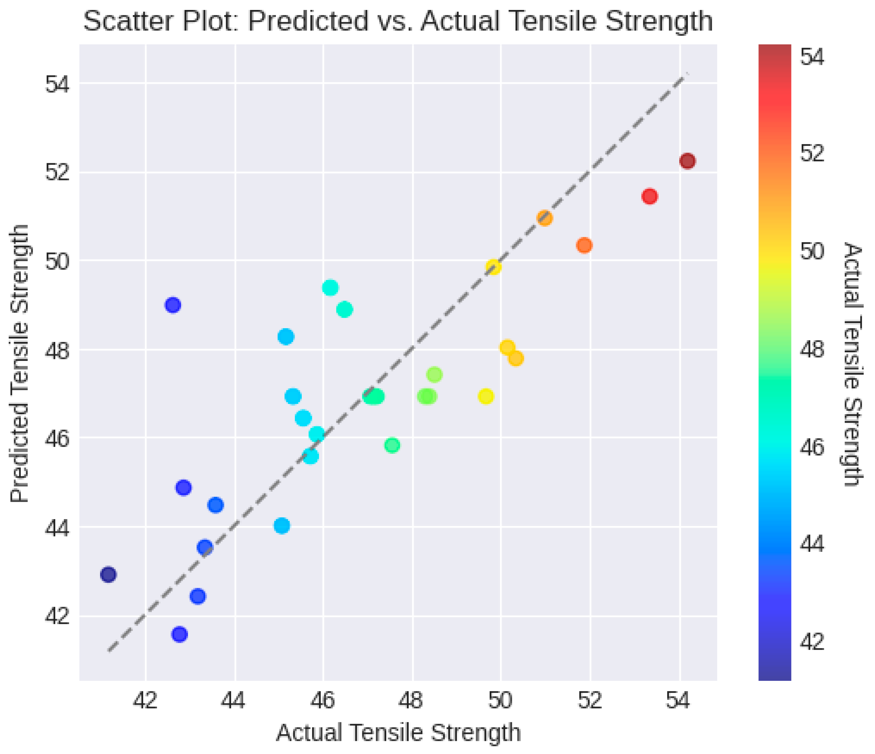
The scatter plot as shown in Figure 6 allows us to visually assess how well the predicted tensile strengths match the actual (ground truth) tensile strengths. Each point on the plot represents a data point, where the x-coordinate is the actual tensile strength and the y-coordinate is the predicted tensile strength. If the points closely follow a diagonal line (the gray dashed line in the plot), it indicates that the predictions are accurate and closely aligned with the ground truth.

Each point's color corresponds to the real tensile strength value. This color information adds a new level of information dimension. It may be a sign of heteroscedasticity, when prediction errors fluctuate across different levels of actual tensile strength, if the color gradient shifts along the expected vs. actual line.

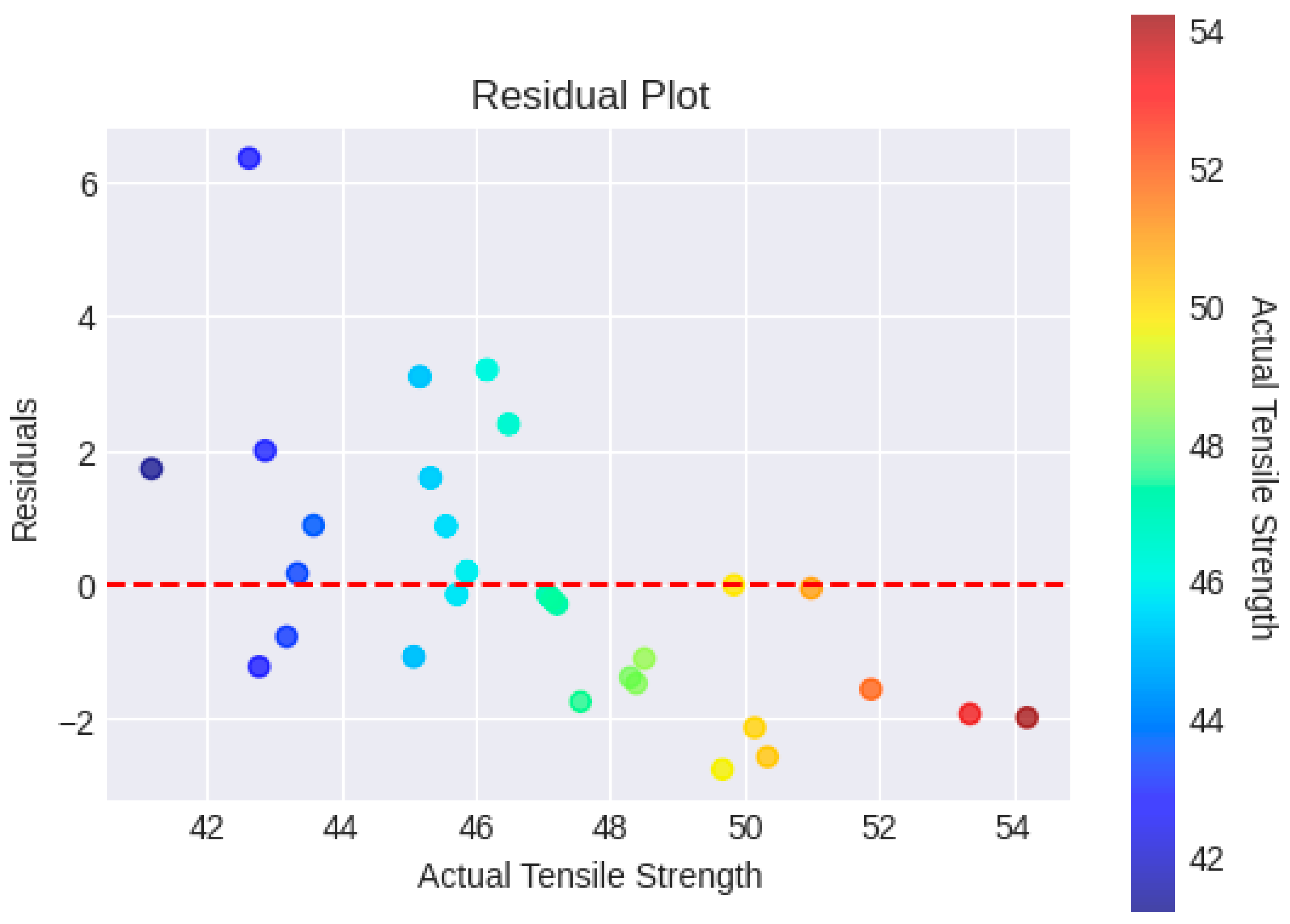
The link between the actual tensile strength values and the related residuals (differences between anticipated and real values) from a machine learning model is depicted in Figure 7 which is a residual plot. We can locate any systematic biases or inaccuracies in the predictions of the model by examining the scatter plot of the actual tensile strength vs. residuals. The residuals may be systematically overestimating or underestimating the tensile strength if they consistently wander above or below the horizontal line (y = 0). The plot reveals how the model's predictive power varies at various levels of observed tensile strength. If a particular pattern can be seen in the residuals (e.g., a rise or drop with increasing tensile strength), the model's performance is not uniform across the whole range of data. As residuals that considerably depart from the horizontal line, outliers or anomalous data points might be found. These points could be examples of situations when the model's predictions were noticeably off or where there were problems with the data.

The model's predictions appear to be impartial and precise because of the random distribution of points around the horizontal line (y = 0). On the other hand, a recognizable pattern or trend in the residuals can suggest that key aspects of the data have been missed by the model.

5. Conclusion

It is clear from the results of using a Graph Neural Network (GNN) to forecast the tensile strength of an additively built specimen that the GNN shown a noteworthy capacity for doing so. Mean absolute error (MAE) of 1.14 and mean squared error (MSE) of 2.47, respectively, indicate that the model produced predictions with relatively low variance. Additionally, the model's capacity to explain almost 78% of the variation in tensile strength observed is highlighted by its R-squared value of 0.78, which demonstrates its strong predictive power. Recognizing that there are still opportunities for improvement and improvement is important. It is acknowledged that more optimization may be possible. The inclusion of additional data, such as material characteristics or manufacturing process factors, into the graph is an attractive area for future exploration. This project tries to determine whether increased information leads to better prediction accuracy. This study lays the groundwork for such iterative improvements by showing the GNN's potential while simultaneously encouraging the investigation of more thorough prediction frameworks.

Author Contributions

Conceptualization, A.M. and V.S.J.; Methodology, A.M.; Software, A.M.; Validation, AM. and V.S.J.; Formal Analysis, V.S.J.; Investigation, A.M.; Resources, V.S.J.; Data Curation, A.M.; Writing – Original Draft Preparation, A.M.; Writing – Review & Editing, V.S.J.; Visualization, A.M.; Supervision, V.S.J.; Project Administration, V.S.J.

Funding Information

No external funding was received for this research work.

Conflict of Interests Statement

The authors declare no competing interest.

References

Zhou, J.; Cui, G.; Hu, S.; Zhang, Z.; Yang, C.; Liu, Z.; Wang, L.; Li, C.; Sun, M. Graph neural networks: A review of methods and applications. AI open 2020, 1, 57–81. [Google Scholar] [CrossRef]
Scarselli, F.; Gori, M.; Tsoi, A.C.; Hagenbuchner, M.; Monfardini, G. The graph neural network model. IEEE transactions on neural networks 2008, 20, 61–80. [Google Scholar] [CrossRef] [PubMed]
Shchur, O.; Mumme, M.; Bojchevski, A.; Günnemann, S. Pitfalls of graph neural network evaluation. arXiv arXiv:1811.05868, 2018.
Xu, K.; Hu, W.; Leskovec, J.; Jegelka, S. How powerful are graph neural networks? arXiv arXiv:1810.00826, 2018.
Liu, M.; Gao, H.; Ji, S. Towards deeper graph neural networks. Proceedings of the 26th ACM SIGKDD international conference on knowledge discovery & data mining (pp. 338-348). 2020 August.
Zheng, X.; Liu, Y.; Pan, S.; Zhang, M.; Jin, D.; Yu, P.S. Graph neural networks for graphs with heterophily: A survey. arXiv arXiv:2202.07082, 2022.
Wu, L.; Chen, Y.; Shen, K.; Guo, X.; Gao, H.; Li, S.; Pei, J.; Long, B. Graph neural networks for natural language processing: A survey. Foundations and Trends® in Machine Learning 2023, 16, 119–328. [Google Scholar] [CrossRef]
Xia, L.; Liang, Y.; Leng, J.; Zheng, P. Maintenance planning recommendation of complex industrial equipment based on knowledge graph and graph neural network. Reliability Engineering & System Safety 2023, 232, 109068. [Google Scholar]
Liu, X.; Li, X.; Fiumara, G.; De Meo, P. Link prediction approach combined graph neural network with capsule network. Expert Systems with Applications 2023, 212, 118737. [Google Scholar] [CrossRef]
Hestroffer, J.M.; Charpagne, M.A.; Latypov, M.I.; Beyerlein, I.J. Graph neural networks for efficient learning of mechanical properties of polycrystals. Computational Materials Science 2023, 217, 111894. [Google Scholar] [CrossRef]
Mozaffar, M.; Liao, S.; Lin, H.; Ehmann, K.; Cao, J. Geometry-agnostic data-driven thermal modeling of additive manufacturing processes using graph neural networks. Additive Manufacturing 2021, 48, 102449. [Google Scholar] [CrossRef]
Badini, S.; Regondi, S.; Lammi, C.; Bollati, C.; Donvito, G.; Pugliese, R. Computational Mechanics of Form-Fitting 3D-Printed Lattice-Based Wrist-Hand Orthosis for Motor Neuron Disease. Biomedicines 2023, 11, 1787. [Google Scholar] [CrossRef] [PubMed]
Sala, R.; Regondi, S.; Graziosi, S.; Pugliese, R. Insights into the printing parameters and characterization of thermoplastic polyurethane soft triply periodic minimal surface and honeycomb lattices for broadening material extrusion applicability. Additive Manufacturing 2022, 58, 102976. [Google Scholar] [CrossRef]
Xu, Z.; La Mendola, I.; Razavi, S.M.J.; Bagherifard, S. Additive manufactured Triply Periodical Minimal Surface lattice structures with modulated hybrid topology. Engineering Structures 2023, 289, 116249. [Google Scholar] [CrossRef]
Greco, L.; Buccino, F.; Xu, Z.; Vergani, L.; Berto, F.; Guagliano, M.; Razavi, S.M.J.; Bagherifard, S. Design and analysis of energy absorbent bioinspired lattice structures. Journal of Bionic Engineering 2023, 1–17. [Google Scholar] [CrossRef]

Figure 1. Prepared samples in the present work

Figure 2. FDM Process setup

Figure 3. Framework used in the present work

Figure 4. Adjacency Matrix plot

Figure 5. Variation of learning rate with number of epochs

Figure 6. Plot for Predicted vs Actual Tensile Strength

Figure 7. Residual plot obtained in the present work

Table 1. Experimental Results

Infill percentage	Layer height (mm)	Print speed (mm/s)	$Extrusion temperature (℃$ )	Tensile strength (MPa)
78	0.32	35	220	46.17
10.5	0.24	50	210	42.78
33	0.16	35	220	45.87
33	0.32	35	200	41.18
33	0.16	65	200	43.59
100	0.24	50	210	54.2
78	0.16	35	200	51.88
33	0.32	65	200	43.19
78	0.32	65	200	50.34
33	0.16	65	220	45.72
78	0.16	35	220	53.35
55.5	0.24	50	210	49.67
33	0.32	35	220	45.08
55.5	0.24	50	190	47.56
55.5	0.24	50	210	48.39
78	0.32	65	220	46.49
55.5	0.24	50	210	47.21
55.5	0.24	50	210	48.3
55.5	0.24	50	230	50.15
33	0.32	65	220	43.35
55.5	0.24	50	210	45.33
55.5	0.24	80	210	45.56
78	0.16	65	200	49.84
55.5	0.24	20	210	48.51
55.5	0.08	50	210	42.63
55.5	0.4	50	210	42.87
55.5	0.24	50	210	47.14
78	0.32	35	200	45.17
55.5	0.24	50	210	47.07
78	0.16	65	220	50.99
33	0.16	35	200	52.87

Table 2. Obtained Metrics features

MSE	MAE	R²
2.47	1.14	0.78

Disclaimer/Publisher’s Note: The statements, opinions and data contained in all publications are solely those of the individual author(s) and contributor(s) and not of MDPI and/or the editor(s). MDPI and/or the editor(s) disclaim responsibility for any injury to people or property resulting from any ideas, methods, instructions or products referred to in the content.

© 2023 by the authors. Licensee MDPI, Basel, Switzerland. This article is an open access article distributed under the terms and conditions of the Creative Commons Attribution (CC BY) license (https://creativecommons.org/licenses/by/4.0/).

Copyright: This open access article is published under a Creative Commons CC BY 4.0 license, which permit the free download, distribution, and reuse, provided that the author and preprint are cited in any reuse.

MDPI Initiatives

Important Links

Choose an area of interest and we will send you notifications of new preprints at your preferred frequency.

Disclaimer

Graph Neural Networks (GNN) for Tensile Strength Prediction in Additive Manufacturing

Abstract

1. Introduction

2. Problem Statement

3. Experimental Procedure

4. Results and Discussion

5. Conclusion

Author Contributions

Funding Information

Conflict of Interests Statement

References

MDPI Initiatives

Important Links

Subscribe