Generalized Rough Neighborhood Approximations and Related Topological Approaches

Preprint

Article

Generalized Rough Neighborhood Approximations and Related Topological Approaches

This version is not peer-reviewed.

Amgad Salem Salama^*

Abdelfattah A. El-Atik,Ali Hussein Salem,Osamy Embaby,

Mona Samy Bondok^*

Amgad Salem Salama^*

Abdelfattah A. El-Atik,Ali Hussein Salem,Osamy Embaby,

Mona Samy Bondok^*

This version is not peer-reviewed.

Altmetrics

Downloads

165

Views

Comments

Submitted:

13 August 2023

Posted:

15 August 2023

You are already at the latest version

Abstract

This work aims to generate some types of M_(j )–neighborhoods. Relationships among these M_(j )-neighborhoods and some other types of neighborhoods are discussed. Additionally, M_(j )-lower, M_(j )-upper approximations and M_(j )-accuracy in terms of M_(j )-neighborhoods are presented. Their properties, with some examples, are investigated. Finally, We addressed the comparisons among M_(j )approach and other approaches.

Keywords:

Subject:

Computer Science and Mathematics - Information Systems

1. Introduction

Topology and rough sets are two distinct mathematical frameworks, but many con nections exist. Rough set theory [1,2,3,4,5] is a good non-statistical tool for big data. It depends essentially on binary relations that are equivalence. These types of relations are often hard to satisfy because of their restrictions and application limitations. The philosophy of rough set theory depends on two approximations of categories. This theory can extend to many other approaches related to topological notations, such as near-open sets and neighborhoods. Topology is an important branch of mathematics that is rich with logical relations. These relations can make use of many generalizations and useful applications. It has many near-open logical notations, such as alpha and beta open sets, that generate new real-life applications. More studies had done to use topology with rough set theory in different ways [6,7,8,9,10,11]. Topologically, rough approximations are motivated by different types of neighborhoods. Some studies [12,13,14,15] used generalized binary relations to generate new rough-set approaches. Others used topological neighborhood systems to generate granules used in many applications [16,17,18,19]. Also, some introduced a mixed neighborhood system for rough approximations and developed eight different types of neighborhoods. These types of neighborhood systems are studied and generalized by to

P_{j}

-neighborhoods,

E_{j}

-neighborhoods,

C_{j}

-neighborhoods, and recently

S_{j}

-neighborhoods. The connection between rough set theory and topology is studied in various directions depending on the suitable applications [8]. The following manuscript is formulated as follows: Sections 1&2 are the introduction and preliminaries of the work. Section 3 introduces the concepts of

M_{j}

neighborhoods systems. Section 4 introduces the relations between these neighborhoods, and Section 5 communicates and revision the notions

M_{j}

-lower and

M_{j}

-upper approximations,

M_{j}

-boundary region,

M_{j}

-positive and

M_{j}

-negative regions, and

M_{j}

-accuracy measure, and generate their

M_{j}

–topologies in section 6. We studied the relations among the generated topologies in Section 7. Some approximations operators induced by the topologies

τ_{M_{j}}

studied in Section 8, and we investigate the concepts from a topological concept, and its main properties are explored. Moreover, Section 9 compares our approaches and previous approaches concerning different j types. Finally, we give a conclusion in Section 10.

2. Preliminaries

We rewrite some important definitions and notations for non-specific readers to help them read this work easily. These definitions spotlight on different types of neighborhoods and relations.

2.1. Pawlak Approximation Space

Definition 2.1.1. [1,20] The relation

Q

on universe

U

is a subset of

U \times U

. Two elements, p and r, are in relation (in symbols

p Q r

) when (p, r)

\in Q

. The relation

Q

is called:

Reflexive if pQp for each p $\in$ U.
Symmetric if pQr↔rQp.
Transitive if pQn whenever pQr and rQn.
Equivalence is when it is reflexive, transitive, and symmetric.

Definition 2.1.2. [1,20] We assume Q is an equivalence relation. A pair (U, Q) is called an approximation space, where U is the universe, and Q is an equivalence relation on U. Let P be a subset of U, i.e., P

\subseteq

U. Our goal is to characterize the set P concerning Q.

$\underline{Q} (P)$ = $\cup^{}$ { V $\in U$ | V $\subseteq$ P}.
$\bar{Q} (P)$ = $\cup^{}$ { V $\in$ U | V ∩ P ≠ $\emptyset$ }.

The two sets

\underline{Q} (P)

and

\bar{Q} (P)

are respectively called lower and upper approximations of P, and P is said to be a rough set if

\underline{Q} (P) \neq \bar{Q} (P)

. Otherwise, it is definable (or exact).

The boundary and accuracy of Pawlak approximations are defined, respectively, by:

BND(P) = $\bar{Q} (P)$ − $\underline{Q} (P)$ and $μ (P)$ = $\frac{| \underline{Q} (P) |}{| \bar{Q} (P) |}$ , Where $\bar{Q} (P) \neq \emptyset$ .

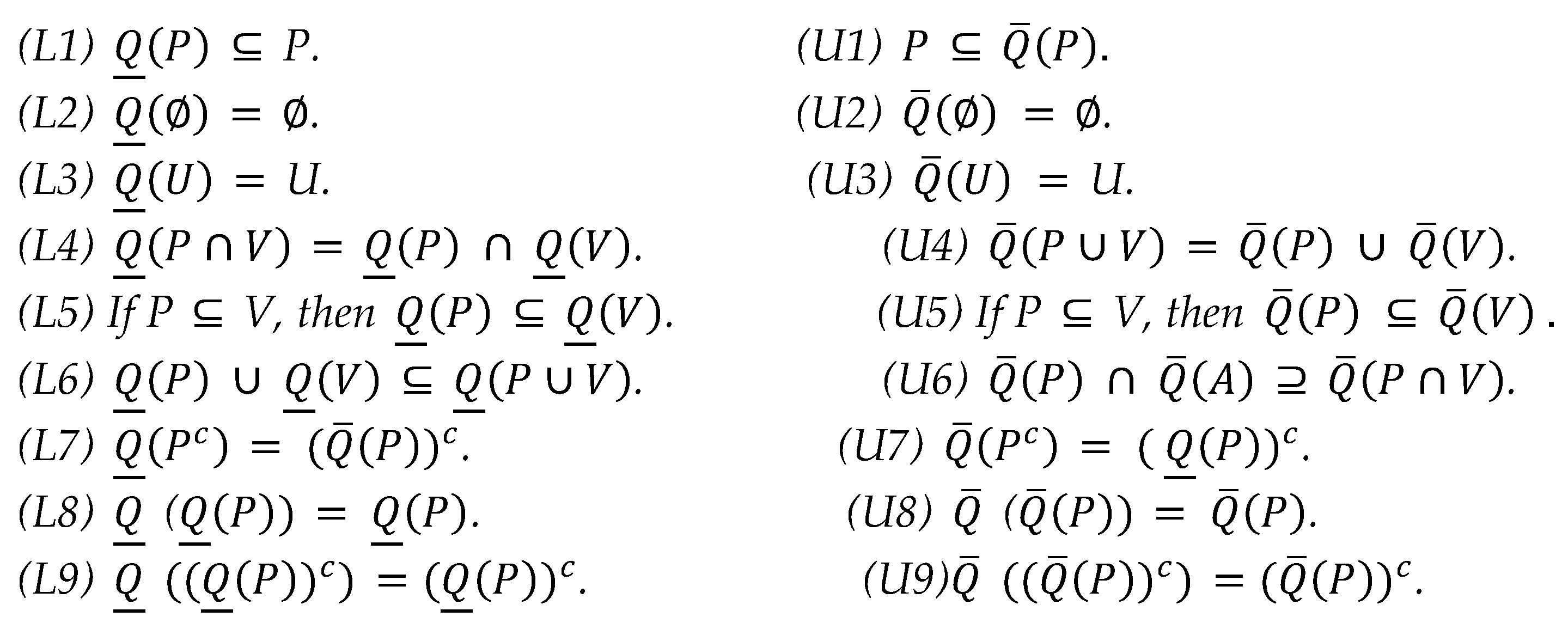
Proposition 2.1.1. [1,20] Pawlak supposes that (U, Q) be an approximation space,

\emptyset

represents an empty set and

P^{c}

represents a complement of P in U. Then, the lower approximations and the upper approximations have the followings properties:

2.2. j-Neighborhood space

Definition 2.2.1. [12] For any binary relation Q on U. The following j-neighborhood sets are defined for p

\in

∪ (

N_{j}

(p)), j

\in

{r, l, ‹ r ›, ‹ l ›, i, u, ‹ i ›, ‹ u ›} as follows:

The r-Neighborhood when, $N_{r}$ (p) = {v $\in$ U | p Q v}.
The l-Neighborhood when, $N_{l}$ (p) = {v $\in$ U | v Q p}.
The ‹ r ›-Neighborhood when, $N_{‹ r ›}$ (p) = ${\cap^{}}_{p \in N_{r} (v)} N_{r}$ (v).
The ‹ l ›-Neighborhood when, $N_{‹ l ›}$ (p) = ${\cap^{}}_{p \in N_{l} (v)} N_{l}$ (v).
The i-Neighborhood when, $N_{i}$ (p) = $N_{r}$ (p) ∩ $N_{l}$ (p).
The u-Neighborhood when, $N_{u}$ (p) = $N_{r}$ (p)∪ $N_{r}$ (p).
The ‹ i ›-Neighborhood when, $N_{‹ i ›}$ (p) = $N_{‹ r ›}$ (p) ∩ $N_{‹ l ›}$ (p).
The ‹ u ›-Neighborhood when, $N_{‹ u ›}$ (p) = $N_{‹ r ›}$ (p)∪ $N_{‹ l ›}$ (p).

Definition 2.2.2. [12] Let Q be an arbitrary binary relation on U and ξj : U→ P(U) be a mapping which assigns for each p

\in

U its

N_{j}

(p) in the P(U) . Then, the triple (U, Q, ξj ) called a j-neighborhood space (briefly, j-NS).

Theorem 2.2.1. [12] Let (U, Q, ξj ) be a j-NS and P

\subseteq

U. Then, for each j

\in

{r, l, ‹ r ›, ‹ l ›, i, u, ‹ i ›, ‹ u ›}the group

τ_{j}

= {

P \subseteq U | \forall v \in P, N_{j}

(v)

\subseteq

P} is a topology on U.

Definition 2.2.3. [12] Let (U, Q, ξj ) be a j-NS. Then, a subset P

\subseteq

U is called a j-open set if P

\in

τ_{j}

. The complement of a j-open set is called j-closed, and the family

Г_{j}

of all j-closed sets is given by

Г_{j} =

{ F

\subseteq U

F^{c} \in τ_{j}

} and the j-interior (resp. j-closure) operator of A is given by

$i n t_{j} (P)$ = ∪ {G $\in τ_{j}$ : G $\subseteq$ P}.
$c l_{j} (P)$ = $\cap^{}$ { H $\in τ^{c}_{j}$ : P $\subseteq$ H}.

Definition 2.2.4. [12] Let (U, Q, ξj ) be a j-NS and P

\subseteq

U. Then, the (j-lower and j-upper) approximations, (j-boundary, j-positive and j-negative) regions, and j-accuracy of the approximations of P

\subseteq

U are given, respectively, by

${\underline{Q}}_{j}$ (P) = ∪ { G $\in τ_{j}$ : G $\subseteq$ P } = j-interior of P.
${\bar{Q}}_{j}$ (P) = $\cap^{}$ { H $\in τ_{j}$ : P $\subseteq$ H } = j-closure of P.
$B_{j} (P)$ = ${\bar{Q}}_{j}$ (P) _ ${\underline{Q}}_{j}$ (P).
$P O S_{j}$ (P) = ${\underline{Q}}_{j}$ (P).
$N E G_{j} (P)$ = $U - {\underline{Q}}_{j}$ (P).
$μ_{j} (P)$ = $\frac{| {\underline{Q}}_{j} (P) |}{| {\bar{Q}}_{j} (P) |}$ , where $| {\bar{Q}}_{j} (P) | \neq 0.$

Definition 2.2.5. [18] For any binary relation Q on U. The group of

E_{j}

-neighborhoods of P

\subseteq

U are defined as follows:

$E_{r}$ (P) = {v $\in$ U: $N_{r}$ (v) ∩ $N_{r}$ (P) ≠∅}.
$E_{l}$ (P) = {v $\in$ U: $N_{l}$ (v) ∩ $N_{l}$ (P) ≠∅}.
$E_{i}$ (P) = $E_{r}$ (P) ∩ $E_{l}$ (P).
$E_{u}$ (P) = $E_{r}$ (P) ∪ $E_{l}$ (P).
$E_{‹ r ›}$ (P) = {v∈U: $N_{‹ r ›}$ (v) ∩ $N_{‹ r ›}$ (P) ≠∅}.
$E_{‹ l ›}$ (P) = {v∈U $: N_{‹ l ›}$ (v) ∩ $N_{‹ l ›}$ (P) ≠∅}.
$E_{‹ i ›}$ (P) = $E_{‹ r ›}$ (P) ∩ $E_{‹ l ›}$ (P).
$E_{‹ u ›}$ (P) = $E_{‹ r ›}$ (P) ∪ $E_{‹ l ›}$ (P).

3. M_{j}_{}

-Neighborhoods in the j -neighborhood space

In this section, we define the concepts of

M_{j}

neighborhoods By inclusion relations between

N_{j}

-neighborhoods and

E_{j}

-neighborhoods. An illustrative example is given to support the obtained results and relationships. The study of

M_{j}

-neighborhoods aims to increase the accuracy of approximations.

Definition 3.1. For any binary relation Q on U. The class of

M_{j}

-neighborhoods of P

\in

U (

M_{j}

(P)) are defined, for each

j \in {r, l, i, u, ‹ r ›, ‹ l ›, ‹ i ›, ‹ u ›}

as follows:

$M_{r}$ (P) = { v $\in$ U: $N_{r}$ (P) $\cap^{}$ $E_{r}$ (P) }.
$M_{l}$ (P) = { v $\in$ U: $N_{L}$ (P) $\cap^{}$ $E_{l}$ (P) }.
$M_{i}$ (P) = ${v \in U : M_{r} (P) \cap^{} M_{l} (P)} .$
$M_{u}$ (P) = ${v \in U : M_{r} (P) \cup^{} M_{l} (P)}$ .
$M_{‹ r ›}$ (P) = { v $\in$ U: $N_{‹ r ›}$ (P) $\cap^{}$ $E_{‹ r ›} (P)$ }.
$M_{‹ l ›}$ (P) = { v $\in$ U $: N_{‹ l ›}$ (P) $\cap^{}$ $E_{‹ l ›}$ (P)}.
$M_{‹ i ›}$ (P) = { v $\in$ U $: M_{‹ r ›}$ (P) $\cap^{}$ $M_{‹ l ›}$ (P)}.
$M_{‹ u ›}$ (P) = ${v \in U : M_{‹ r ›} (P) \cup^{} M_{‹ l ›} (P)} .$

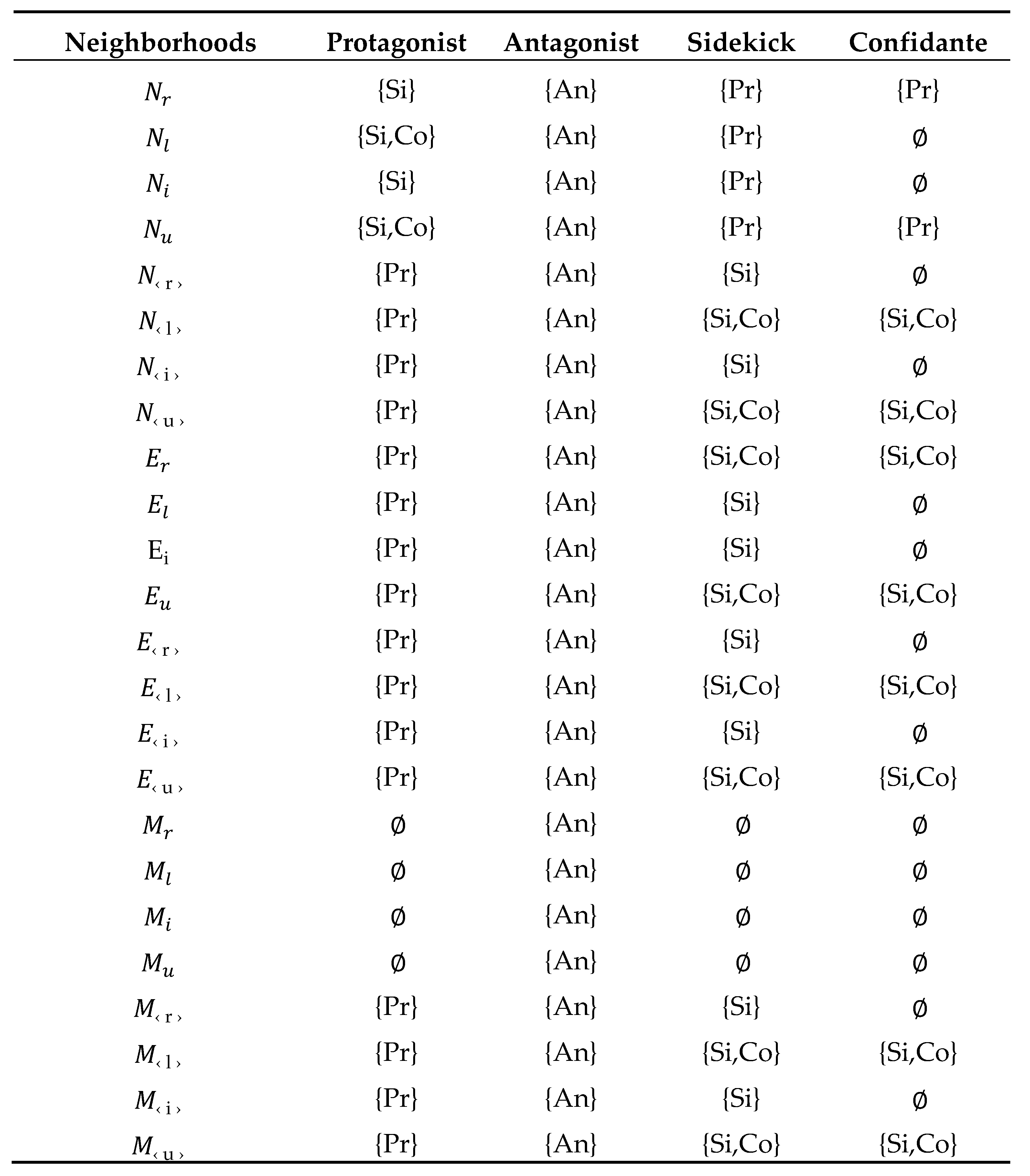
The following example will show the behavior of these neighborhoods, help us show the relationships among them, and illustrates the method of Mj-neighborhood.

Example 3.1. Suppose the universe of some types of characters in a story

U = {P r o t a g o n i s t (P r), A n t a g o n i s t (A n), S i d e k i c k (S i), C o n f i d a n t e (C o)}

as an initial set of objects. We suppose the relation

Q = {(P r, S i), (A n, A n), (S i, P r), (C o, P r)}

that defined on U. The classes

N_{j}

neighborhoods,

E_{j}

-neighborhoods and

M_{j}

-neighborhoods are shown inTable 1.

4. The Relationships Among $M_{j}$ –neighborhoods

The following results show the relationships between the different types of Mj-neighborhoods.

Proposition 4.1. Let (U, Q, ξj) be a j-approximation space. Then for each v

\in U,

the following relations hold.

v $\in$ (v) for each j.
$M_{i}$ (v) $\subseteq$ $M_{r}$ (v) $\subseteq$ $M_{u}$ (v).
$M_{i}$ (v) $\subseteq$ $M_{l}$ (v) $\subseteq$ $M_{u}$ (v).
$M_{‹ i ›}$ (v) $\subseteq$ $M_{‹ r ›}$ (v) $\subseteq$ $M_{‹ u ›}$ (v).
(v) $\subseteq$ $M_{‹ l ›}$ (v) $\subseteq$ $M_{‹ u ›}$ (v).
If Q is symmetric, then $M_{r}$ (v) = $M_{l}$ (v) = $M_{i}$ (v) $= M_{u}$ (v) and $M_{‹ r ›}$ (v) = $M_{‹ l ›}$ (v)= $M_{‹ i ›}$ (v) $=$ $M_{‹ u ›}$ (v).

Proof. The proof of (1) comes from the fact

N_{j}

(v)

\subseteq N_{j}

(v) and

E_{j}

(v)

\subseteq E_{j}

(v) for

j \in {r, l, ‹ r ›, ‹ l ›}

The proof of (2)-(5) come from the Definition 3.1.

The proof of (6): Since Q is symmetric, then

N_{r}

(v) =

N_{l}

(v). This leads to

N_{i}

(v)

= N_{u}

(v) as well and

E_{r}

(v) =

E_{l}

(v). This leads to

E_{i}

(v)

= E_{u}

(v). Therefore,

M_{r}

(v) =

M_{l}

(v) =

M_{i}

(v)

= M_{u}

(v) . Similarly, one can prove that and

M_{‹ r ›}

(v) =

M_{‹ l ›}

(v) =

M_{‹ i ›}

(v)

=

M_{‹ u ›}

(v). □

5. Generalized Rough Approximations Based on $M_{j}$ –neighborhoods

In this section, New concepts of

M_{j}

-lower approximations and

M_{j}

-upper approximations,

M_{j}

-boundary region,

M_{j}

–positive regions,

M_{j}

-negative regions and

M_{j}

-accuracy measure of a subset based on

M_{j}

–neighborhoods. We reveal the main properties with the help of some examples.

Definition 5.1. Let (U, Q, ξj) be a j-approximation Space, given a set P

\subseteq

U. The lower

Ƃ_{M_{j}}

(P) and the upper

Ƃ^{M_{j}}

(P) approximations based on

M_{j}

-neighborhoods defined as follows:

$Ƃ_{M_{j}}$ (P) = { v $\in$ U , $M_{j}$ (v) $\subseteq$ P } Called $M_{j}$ lower approximation of P.
$Ƃ^{M_{j}}$ (P) = { v $\in$ U , $M_{j}$ (v) $\cap^{}$ P ≠ $\emptyset$ } Called $M_{j}$ upper approximation of P.

Definition 5.2. Let (U, Q, ξj) be a j-approximation Space, given a set P

\subseteq

U. The

M_{j}

-boundary region,

M_{j}

-positive region,

M_{j}

-negative region and

M_{j}

-accuracy of P is defined as follows:

$B_{M_{j}} (P)$ = $Ƃ^{M_{j}}$ (P) _ $Ƃ_{M_{j}}$ (P)
${POS}_{M_{j}}$ (P) = $Ƃ_{M_{j}}$ (P)
${NEG}_{M_{j}}$ (P) = $U - Ƃ^{M_{j}}$ (P)
$δ_{M_{j}} (P)$ = $\frac{| Ƃ_{M_{j}} (P)_{|}}{| Ƃ^{M_{j}} (P) |}$ , where $| Ƃ^{M_{j}} (P) | \neq 0.$

In the next example, we calculate the

M_{j}

lower approximation of P,

M_{j}

upper approximation of P,

M_{j}

-boundary region,

M_{j}

-positive region,

M_{j}

-negative region and

M_{j}

-accuracy measure of P.

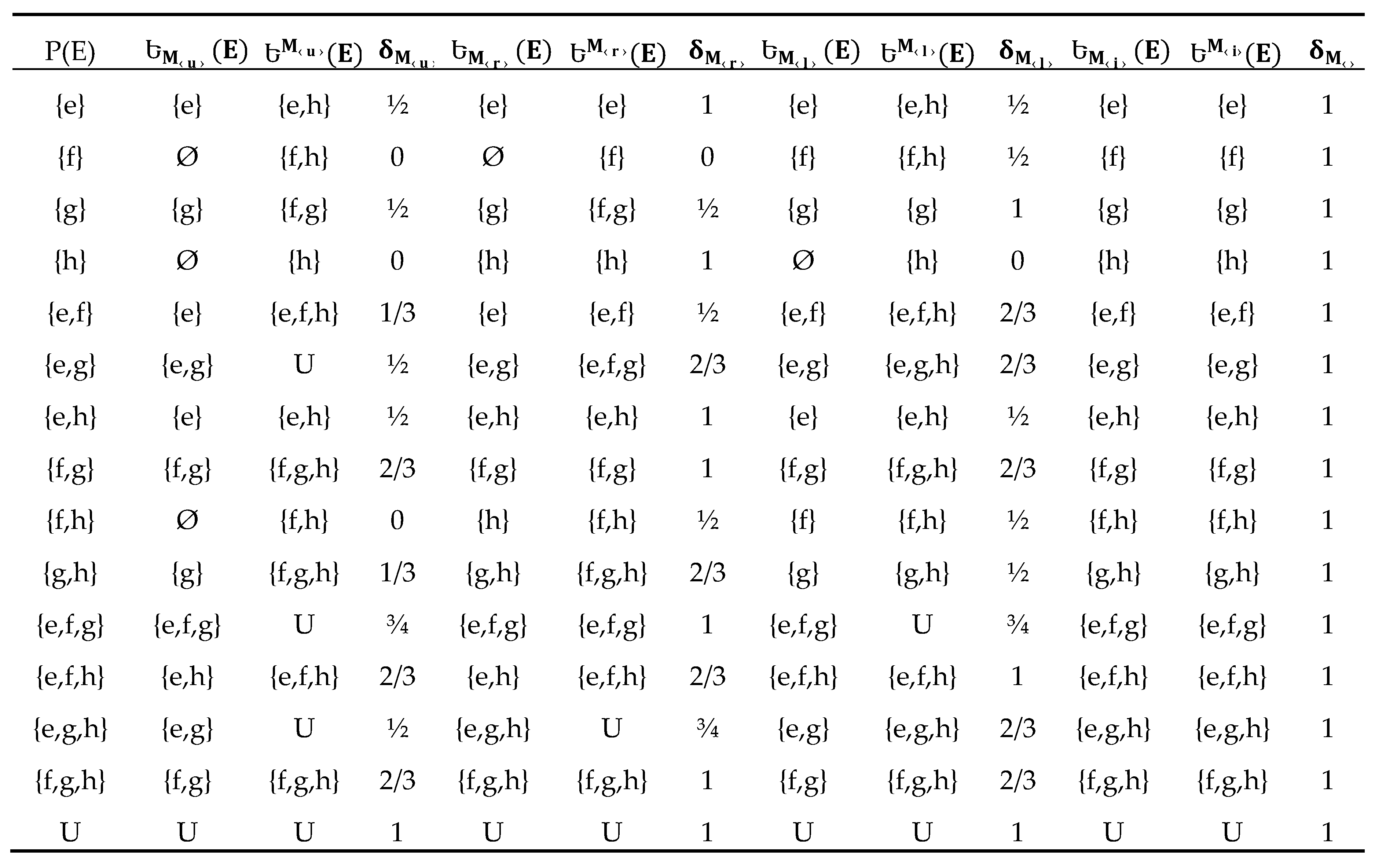
Example 5.1. Suppose the universe U= {e, f, g, h} as an initial set of objects and P

\subseteq

U. We suppose the relation Q = {(e,e),(e,h),(f,e),(f,g),(g,f),(g,g),(g,h),(h,e)} that defined on U.

Let P ={e,f,h}. Then we calculate

Ƃ_{M_{j}}

(P),

Ƃ^{M_{j}}

(P),

F_{M_{j}} (P)

and

δ_{M_{j}} (P)

for j=(r,l,i,u) as follows:

For j = r, we have $Ƃ_{M_{r}}$ (P) ={e,h} , $Ƃ^{M_{r}}$ (P) = U, $F_{M_{r}} (P) =$ {f,g} and $δ_{M_{r}} (P)$ = ½.
For j = l, we have $Ƃ_{M_{l}}$ (P) ={e} , $Ƃ^{M_{l}}$ (P) = {e,g,h}, $F_{M_{l}} (P) =$ {g,h} and $δ_{M_{l}} (P)$ = 1/3.
For j = i, we have $Ƃ_{M_{i}}$ (P) ={e,h} , $Ƃ^{M_{i}}$ (P) = {e,g,h}, $F_{M_{i}} (P) =$ {g} and $δ_{M_{i}} (P)$ = 2/3
For j = u, we have $Ƃ_{M_{u}}$ (P) ={e} , $Ƃ^{M_{u}}$ (P) = U, $F_{M_{u}} (P) =$ {f,g,h} and $δ_{M_{u}} (P)$ = 1/3.

Proposition 5.1. For any j and each non-empty subset P of U, we have

δ_{M_{j}} (P)

\in

[0,1].

Proof. Let P be a non-empty subset of U. It follows from (1) of Proposition 4.1 that v

\in

M_{j}

(v) for each j. Then

M_{j}

(v)

\cap^{​} P

\neq

\emptyset

for each v

\in

P; consequently,

Ƃ^{M_{j}}

(P)

\neq

\emptyset

. Thus,

| Ƃ^{M_{j}} (P) | > 0

. □

Now, we have two cases:

Case 1:

Ƃ_{M_{j}}

(P) =

\emptyset

. Then

\frac{| Ƃ_{M_{j}} (P)_{|}}{| Ƃ^{M_{j}} (P) |} = \frac{| \emptyset |}{| Ƃ^{M_{j}} (P) |}

= 0.

Case 2:

Ƃ_{M_{j}} (P) \neq

\emptyset

. Then v

\in

Ƃ_{M_{j}}

(P). Then v

\in

M_{j}

(v)

\cap^{​} P

. Therefore, v

\in

Ƃ^{M_{j}}

(P). Thus

Ƃ_{M_{j}}

(P)

\subseteq

Ƃ^{M_{j}}

(P). This means that 0 ≤

\frac{| Ƃ_{M_{j}} (P)_{|}}{| Ƃ^{M_{j}} (P) |}

≤ 1. Hence, we obtain from the two cases above that 0 ≤

δ_{M_{j}} (P)

≤ 1 as required.

In the following results, we present the main properties of

M_{j}

-lower approximations and

M_{j}

-upper approximations for each j.

Theorem 5.2. Let (U, Q, ξj) be a j-approximation space, given a set P

\subseteq

U. Then the following properties hold for each j.

$Ƃ_{M_{j}}$ (P) $\subseteq$ P $\subseteq$ $Ƃ^{M_{j}} (P) .$
$Ƃ_{M_{j}}$ ( $\emptyset$ ) = $\emptyset$ and $Ƃ^{M_{j}} (\emptyset)$ = $\emptyset$ .
$Ƃ_{M_{j}}$ (U) = U and $Ƃ^{M_{j}} (U)$ = U.
If P $\subseteq$ W, then $Ƃ_{M_{j}}$ (P) $\subseteq$ $Ƃ_{M_{j}}$ (W) .
If P $\subseteq$ W, then $Ƃ^{M_{j}} (P) \subseteq$ $Ƃ^{M_{j}} (W) .$
$Ƃ_{M_{j}}$ (P $\cap^{}$ W) = $Ƃ_{M_{j}}$ (P) $\cap^{}$ $Ƃ_{M_{j}}$ (W).
$Ƃ^{M_{j}}$ (P ∪W) = $Ƃ^{M_{j}}$ (P) $\cup^{}$ $Ƃ^{M_{j}}$ (W .
$Ƃ_{M_{j}}$ ( $P^{c}$ ) = ${(Ƃ^{M_{j}} (P))}^{C}$ .
$Ƃ^{M_{j}}$ ( $P^{c}$ ) = ${(Ƃ_{M_{j}} (P))}^{C}$ .

Proof. We prove (1) ,(2),(3),(4),(6) and (8) and the other cases similarly.

Let v $\in$ $Ƃ_{M_{j}}$ (P) . Then $M_{j}$ (v) $\subseteq$ P. It follows from the item (1) of Proposition 4.1 that v $\in$ $M_{j}$ (v) therefore, v $\in$ P. Thus, $Ƃ_{M_{j}}$ (P) $\subseteq$ P.
Since $M_{j}$ (v) $\neq$ $\emptyset$ . For each v $\in$ U, then $Ƃ_{M_{j}}$ ( $\emptyset$ ) = $\emptyset$ .
Since v $\in$ $M_{j}$ (v) $\subseteq$ U for each v $\in$ U, then ${\cup^{}}_{v \in U}$ {v} $\subseteq {\cup^{}}_{v \in U}$ $M_{j}$ (v) $\subseteq$ U thus $Ƃ_{M_{j}}$ (U) = U.
Since P $\subseteq$ W, then $Ƃ_{M_{j}}$ (P) = { $v \in Q : M_{j}$ (v) $\subseteq$ P } $\subseteq$ { $v \in Q : M_{j}$ (v) $\subseteq$ W } = $Ƃ_{M_{j}}$ (W).
It follows from (iv) that $Ƃ_{M_{j}}$ (P $\cap^{}$ W) = $Ƃ_{M_{j}}$ (P) $\cap^{}$ $Ƃ_{M_{j}}$ (W). Conversely, let v $\in$ $Ƃ_{M_{j}}$ (P) $\cap^{}$ $Ƃ_{M_{j}}$ (W). Then v $\in$ $Ƃ_{M_{j}}$ (P) and v $\in$ $Ƃ_{M_{j}}$ (W) so that $M_{j}$ (v) $\subseteq$ P and $M_{j}$ (v) $\subseteq$ W thus $M_{j}$ (v) $\subseteq$ P $\cap^{}$ W, Hence v $\in$ $Ƃ_{M_{j}}$ (P $\cap^{}$ W).
v $\in Ƃ_{M_{j}}$ ( $P^{c}$ ) ↔ $M_{j}$ (v) ↔ $M_{j}$ (v) $\cap^{}$ P = $\emptyset$ ↔ v not belong $Ƃ^{M_{j}} (P)$ ↔ v $\in$ ${(Ƃ^{M_{j}} (P))}^{C} .$

Corollary 5.3. Let (U, Q, ξj) be a j-approximation space and P, V

\subseteq

Q. Then

Ƃ_{M_{j}}

(P)

\cup^{​}

Ƃ_{M_{j}}

(V)

\subseteq Ƃ_{M_{j}}

(P V). The next example shows that the converse of the above corollary need not be true.

Example 5.2. According to Example 5.1. Let P = {e}, V = {f, h} and P

\cup^{​}

V = {e,f,h}. Then

Ƃ_{M_{r}}

\cup^{​}

V) ={e},

Ƃ_{M_{r}}

(P) ={e} and

Ƃ_{M_{r}}

(V) =

\emptyset

Ƃ_{M_{r}}

\cup^{​}

⊈ Ƃ_{M_{r}}

(P)

\cup^{​} Ƃ_{M_{r}}

(V).

Remark 5.1. The converse of Theorem 5.2. that

Ƃ_{M_{j}}

(P)

\subseteq

P need not be true. The following example shows this remark.

Example 5.3. According to Example 5.1. Let P = {f, g}, we have

Ƃ_{M_{r}} (p)

= {g} then P

⊈ Ƃ_{M_{j}}

(P).

Remark 5.2. The converse of the item (4) of Theorem 5.2. that If P

\subseteq

W, then

Ƃ_{M_{j}}

(P)

\subseteq

Ƃ_{M_{j}}

(W) need not be true as shown in Example 5.4.

Example 5.4. According to Example 5.1. Let P = {e,f,h} and W = {e,g,h}. Then

Ƃ_{M_{r}}

(P) = {e,h}

\subseteq

Ƃ_{M_{r}}

(W) = {e,f,h} although P

⊈

Some properties of Pawlak’s lower approximations are not realized for

M_{j}

-lower approximation

Ƃ_{M_{j}} (P)

such as

Ƃ_{M_{j}} (Ƃ_{M_{j}} (P)) = Ƃ_{M_{j}} (P)

. To clarify this fact, consider a subset P = {e, f, h}. Then

Ƃ_{M_{u}} (P)

= {e}, But

Ƃ_{M_{j}} (Ƃ_{M_{j}} (P)) = \emptyset

given in Example 5.1.

Corollary5.4. Let (U, Q, ξj) be a j-approximation space and P, V

\subseteq

Q. Then

Ƃ^{M_{j}} (P \cap^{​} V) \subseteq Ƃ^{M_{j}}

(P)

\cap^{​}

Ƃ^{M_{j}}

(V). The next example show that the converse of the above corollary need not be true.

Example 5.5. According to Example 5.1. Let P = {f, h}, V = {e, g, h} and P

\cap^{​}

V = {h}. Then

Ƃ^{M_{l}}

(P) = {e, g},

Ƃ^{M_{l}}

(V) =

U

and

Ƃ^{M_{l}}

\cap^{​}

V) ={e}.

Ƃ^{M_{l}}

(P)

\cap^{​} Ƃ^{M_{l}}

(V)

⊈ Ƃ^{M_{l}}

\cap^{​}

V).

Remark 5.3.The converse or the item (1) of Theorem 5.2. that P

\subseteq

Ƃ^{M_{j}} (P)

Need not be true as shown in the following example.

Example 5.6. According to Example 5.1. Let P = {f, g}, we have

Ƃ^{M_{r}} (p)

={g} then P

⊈ Ƃ^{M_{r}} (p)

Remark 5.4. The converse of item (5) of Theorem 5.2. need not be true as shown in Example 5.7.

Example 5.7. According to Example 5.1. Let P = {g, h} and V = {e,g,h}. Then

Ƃ^{M_{u}} (P)

={e,f,h}

\subseteq

Ƃ^{M_{u}} (V)

= U although P

⊈

Some properties of Pawlak’s upper approximations are not realized for

M_{j}

-Upper approximation

Ƃ^{M_{j}} (P)

such as

Ƃ^{M_{j}} (_{} Ƃ^{M_{j}} (P)) = Ƃ^{M_{j}} (P)

. To clarify this fact, consider a subset P = {f}. Then

Ƃ^{M_{u}} (P)

= {g} But

Ƃ^{M_{u}} (_{} Ƃ^{M_{u}} (P)) = {f, g, h}

given in example 5.1.

Proposition 5.5. Let (U, Q, ξj) be a j-approximation space, given a set P

\subseteq

U. Then the following proposition gives the relationships between the

M_{j}

-lower approximations

Ƃ_{M_{j}}

(P) and

M_{j}

-upper approximations

Ƃ^{M_{j}}

(P) where

j \in {r, l, i, u, ‹ r ›, ‹ l ›, ‹ i ›, ‹ u ›}

$Ƃ_{M_{u}}$ (P) $\subseteq$ $Ƃ_{M_{r}}$ (P) $\subseteq$ $Ƃ_{M_{i}}$ (P) .
$Ƃ_{M_{u}}$ (P) $\subseteq$ $Ƃ_{M_{l}}$ (P) $\subseteq$ $Ƃ_{M_{i}}$ (P) .
$Ƃ_{M_{‹ u ›}}$ (P) $\subseteq$ $Ƃ_{M_{‹ r ›}}$ (P) $\subseteq$ $Ƃ_{M_{‹ i ›}}$ (P)
$Ƃ_{M_{‹ u ›}}$ (P) $\subseteq$ $Ƃ_{M_{‹ l ›}}$ (P) $\subseteq$ $Ƃ_{M_{‹ i ›}}$ (P)
$Ƃ^{M_{i}}$ (P) $\subseteq$ $Ƃ^{M_{r}}$ (P) $\subseteq$ $Ƃ^{M_{u}}$ (P) .
$Ƃ^{M_{i}}$ (P) $\subseteq$ $Ƃ^{M_{l}}$ (P) $\subseteq$ $Ƃ^{M_{u}}$ (P) .
$Ƃ^{M_{‹ i ›}}$ (P) $\subseteq$ $Ƃ^{M_{‹ r ›}}$ (P) $\subseteq$ $Ƃ^{M_{‹ u ›}}$ (P) .
$Ƃ^{M_{‹ i ›}}$ (P) $\subseteq$ $Ƃ^{M_{‹ l ›}}$ (P) $\subseteq$ $Ƃ^{M_{‹ u ›}}$ (P) .

Proof.

We prove (1): Let v $\in$ $Ƃ_{M_{u}}$ (P) then v $\in$ $M_{u}$ (v) $\subseteq$ P. Since $M_{r}$ (v) $\subseteq$ $M_{u}$ (v), then v $\in$ $Ƃ_{M_{r}}$ (P) therefore $Ƃ_{M_{u}}$ (P) $\subseteq$ $Ƃ_{M_{r}}$ (P). □

similarly, we prove that

Ƃ_{M_{r}}

(P)

\subseteq

Ƃ_{M_{i}}

(P) and the other cases (2),(3) and (4) can be proved similarly.

We prove (v): let v $\in$ $Ƃ^{M_{i}} (P)$ then v $\in$ $M_{i}$ (v). Such that $M_{i}$ (v) $\cap^{} P \neq \emptyset$ Since $M_{i}$ (v) $\subseteq$ $M_{r}$ (v). Then $M_{r}$ (v) $\cap^{} P \neq \emptyset$ , therefore $Ƃ^{M_{i}} (P) \subseteq$ $Ƃ^{M_{r}} (P)$ . □

similarly, we prove that

Ƃ^{M_{r}} (P)

\subseteq

Ƃ^{M_{u}} (P)

and the other cases (6),(7) and (8) can be proved similarly.

Proposition 5.6. Let (U, Q, ξj) be a j-approximation space, given a non-empty set P

\subseteq

$δ_{M_{u}} (P) \leq$ $δ_{M_{r}} (P) \leq$ $δ_{M_{i}} (P)$ .
$δ_{M_{u}} (P) \leq$ $δ_{M_{l}} (P) \leq$ $δ_{M_{i}} (P)$ .
$δ_{M_{‹ u ›}} (P)$ $δ_{M_{‹ r ›}} (P) \leq$ $δ_{M_{‹ i ›}} (P)$ .
$δ_{M_{‹ u ›}} (P) \leq$ $δ_{M_{‹ l ›}} (P) \leq$ $δ_{M_{‹ i ›}} (P)$ .

Proof. We prove (1) and one can prove the other cases similarly.

Since

Ƃ_{M_{u}}

(P)

\subseteq

Ƃ_{M_{r}}

(P)

\subseteq

Ƃ_{M_{i}}

(P) then

│ Ƃ_{M_{u}} (P) │

\leq

│ Ƃ_{M_{r}} (P) │ \leq │ Ƃ_{M_{i}} (P) │

Since

Ƃ^{M_{i}}

(P)

\subseteq

Ƃ^{M_{r}}

(P)

\subseteq

Ƃ^{M_{u}}

(P) then

│ Ƃ^{M_{i}} (P) │ \leq

│ Ƃ^{M_{r}} (P) │ \leq

│ Ƃ^{M_{u}} (P) │

By hypothesis, P is non-empty, so that

│ Ƃ^{M_{j}} (P) │

> 0 for each j. Therefore:

\frac{1}{│ Ƃ^{M_{u}} (P) │} \leq

\frac{1}{│ Ƃ^{M_{r}} (P) │} \leq \frac{1}{│ Ƃ^{M_{i}} (P) │}

. Then

\frac{│ Ƃ_{M_{u}} (P) │}{│ Ƃ^{M_{u}} (P) │} \leq

\frac{│ Ƃ_{M_{r}} (P) │}{│ Ƃ^{M_{r}} (P) │} \leq

\frac{│ Ƃ_{M_{i}} (P) │}{│ Ƃ^{M_{i}} (P) │}

. □

To support the above results, we present the following example.

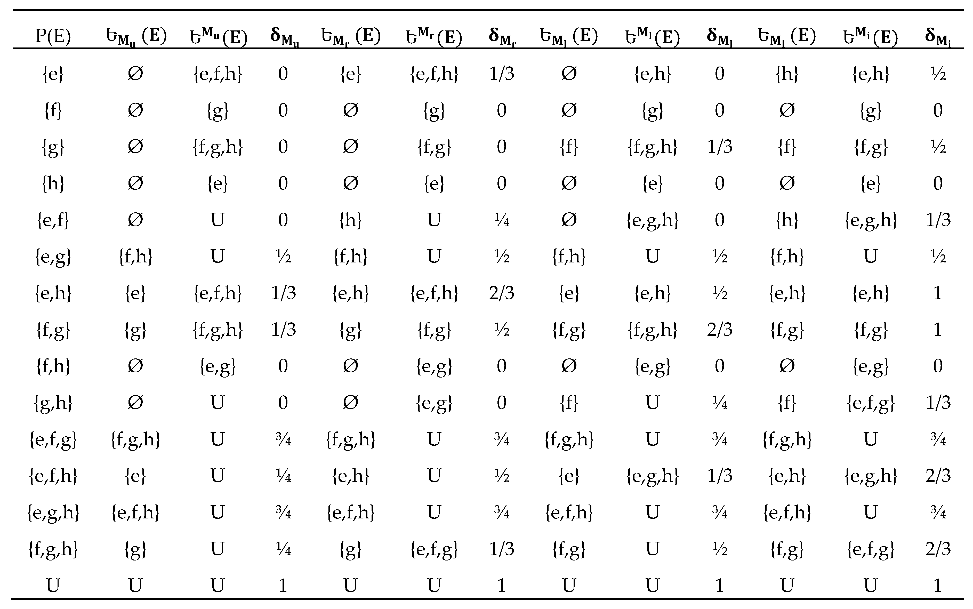
Example 5.8. According to Example 5.1, we calculate the approximations and their accuracy measure for

j \in {r, l, i, u}

as inTable 2, and we calculate the approximations and their accuracy measure

j \in {‹ r ›, ‹ l ›, ‹ i ›, ‹ u ›}

as inTable 3.

M_{j} - T o p l o g i e s

Using the following theorem, we can generate eight different topologies via

M_{j}

-neighborhoods.

Theorem 6.1. If

(U, Q, ξ j)

is a j-approximation space, Then the collection

τ_{M_{j} =} {B \subseteq U | M_{j} (v) \subseteq B f o r a l l v \in B}

f o r j \in {r, l, i, u, ‹ r ›, ‹ l ›, ‹ i ›, ‹ u ›}

is a topology

On U.

Proof.

U and Ø belong to $τ_{M_{j}}$ .
If { $B_{i}$ | i $\in I$ } is a family of elements in $τ_{M_{j}}$ and v $\in$ ${\cup^{}}_{i} B_{i}$ . Then there exists $i_{0} \in I$ such that v $\in$ $B_{i_{0}}$ . Thus, $M_{j}$ (v) $\subseteq$ $B_{i_{0}}$ this lead to $M_{j}$ (v) $\subseteq {\cup^{}}_{i} B_{i}$ and ${\cup^{}}_{i} B_{i} \in$ $τ_{M_{j}}$ .
If $B_{1}, B_{2}$ $\in$ $τ_{M_{j}}$ and P $\in B_{1} \cap^{} B_{2} .$ Then, v $\in B_{1}$ and v $\in$ $B_{2}$ which lead to $M_{j}$ (v) $\subseteq$ $B_{1}$ and $M_{j}$ (v) $\subseteq$ $B_{2}$ Thus, $M_{j}$ (v) $\subseteq$ $B_{1} \cap^{} B_{2}$ and hence $B_{1}, B_{2} \in$ $τ_{M_{j}}$ . Then $τ_{M_{j}}$ is a topology on U. □

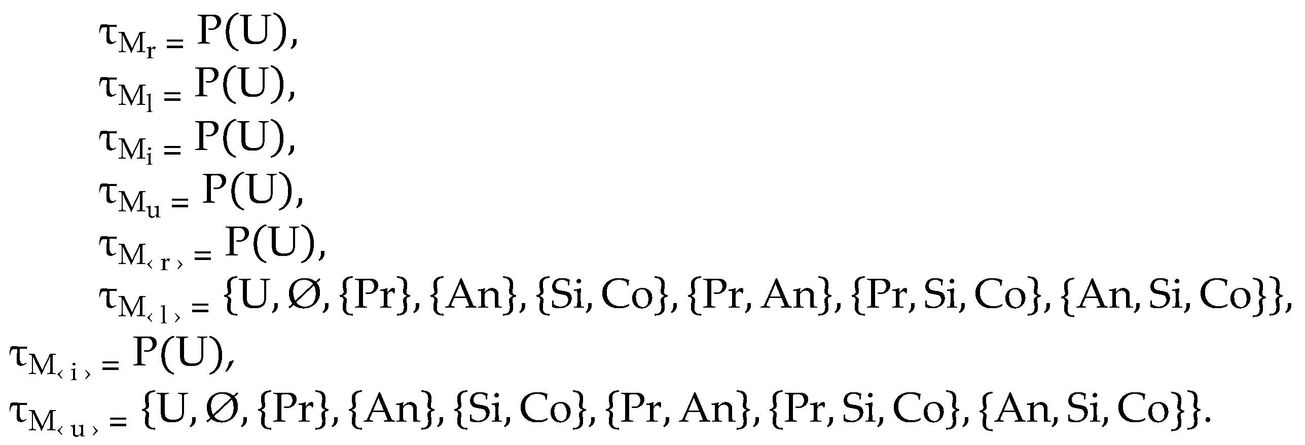
Example 6.1. According to Example 3.1, the classes of

M_{j}

-topologies are given as follows:

7. The Relations Among $τ_{M_{j}}$ Topologies

We study the relationships among the topologies

τ_{M_{r}}

τ_{M_{l}}

τ_{M_{i}}

τ_{M_{u}}

τ_{M_{‹ r ›}}

τ_{M_{‹ l ›}}

τ_{M_{‹ i ›}}

and

τ_{M_{‹ u ›}} .

Proposition 7.1. In a j-NS (U, R, ξj),

τ_{M_{r}}

is the dual topology of

τ_{M_{l}}

Proof. Firstly, let A

\in τ_{M_{r}}

then ∀v

\in

A ,

M_{r}

(v)

\subseteq

A. Suppose that q

\in

B, then

M_{l}

(q)= {y

\in U | y R q}

Now, let

M_{l}

(q) ∩ A ≠

\emptyset

then x ∈ U such that x ∈ A and x ∈

M_{l}

(q) ⇒ x∈A and xRq ⇒ x∈A and q ∈

M_{r}

(x) Since x ∈A ⇒

M_{r}

(x) ⊆ A and so q ∈ A which contradicts with q ∈ B. Thus,

M_{l}

(q) ∩ A =

\emptyset

this implies

M_{l}

(q) ⊆ B. Now, we have ∀q ∈ B,

M_{l}

(q) ⊆ B. Hence, B ∈

τ_{M_{l}}

. Similarly, we can prove that if B ∈

τ_{M_{l}}

. Then,

B^{c}

∈

τ_{M_{r}}

. Consequently,

τ_{M_{r}}

is the dual topology of

τ_{M_{l}} .

□

The following example shows Proposition 7.1

Exemple7.1. Let U = {e, f, g, h} and R = {(e, e),(e, h),(f, e),(f, g),(g, f),(g, g),(g, h),(h, e)}.

Then, we have

τ_{M_{r}}

= {U, Ø, {e, h}},

τ_{M_{l}}

={U,Ø,{f, g}}.

Obviously,

τ_{M_{r}}

is the dual topology of

τ_{M_{l}}

Proposition 7.2. Let (U, Q, ξj) is a j-approximation space , then

τ_{M_{r}}

\subseteq τ_{M_{i}}

τ_{M_{l}}

\subseteq τ_{M_{i}}

Proof. Let B ∈

τ_{M_{r}}

, then ∀ v ∈ B,

M_{r}

(v) ⊆ B. Thus

M_{r}

(v)

\cap^{​}

M_{l}

(v) ⊆ B and so ∀ v ∈ B,

M_{i}

(v) ⊆ B ,Hence B ∈

τ_{M_{i}}

and

τ_{M_{r}}

\subseteq τ_{M_{i}}

, similarly, we can deduce that

τ_{M_{l}} \subseteq τ_{M_{i}}

. □

Remark 7.1. Let (U, R, ξj) be a j-NS and then the following are not necessarily true.

τ_{M_{r}} = τ_{M_{i}}

τ_{M_{l}} = τ_{M_{i}}

Proposition 7.3. Let (U, Q, ξj) is a j-approximation space. Then

τ_{M_{u}} \subseteq τ_{M_{r}}

τ_{M_{u}} \subseteq τ_{M_{l}}

τ_{M_{u}} \subseteq τ_{M_{i}}

Proof. Let B ∈

τ_{M_{u}}

, then ∀ v ∈ B,

M_{u}

(v) ⊆ B. Thus, ∀p ∈ B,

M_{r}

(v) U

M_{l}

(v) ⊆ B and so ∀ v ∈ B,

M_{r}

(v) ⊆ B,

M_{l}

(v) ⊆ B. Then, B ∈

τ_{M_{r}}

and B ∈

τ_{M_{l}}

and

τ_{M_{u}}

⊆

τ_{M_{r}}

and

τ_{M_{u}}

⊆

τ_{M_{l}}

. Using Proposition 7.2. we have

τ_{M_{u}}

⊆

τ_{M_{i}}

. □

Remark 7.2: Let (U, R, ξj) be a j-NS, then the following is not necessarily true.

τ_{M_{u}} = τ_{M_{r}}

τ_{M_{u}} = τ_{M_{l}}

τ_{M_{u}} = τ_{M_{i}}

The following example explains Remark 7.1 and Remark 7.2.

Example 7.2. Let U = {e, f, g, h, k} and R = {(e, e), (f, g), (f, h), (g, h), (g, k), (h, e), (h, k), (k, f), (k, k)}.

Then, we have

τ_{M_{r}}

= {U, Ø, {e},{k},{e, k},{e, h, k},{e, g, h, k}},

τ_{M_{l}}

={U,Ø,{e},{g},{g, h},{g, h, k},{e, g, h, k} {f, g, h, k}}

τ_{M_{i}}

= P(U) and

τ_{M_{u}}

= {U, Ø , {e},{e, g, h, k}}.

Proposition 7.4. Let (U, Q, ξj) is a j-approximation space. Then

τ_{M_{‹ r ›}} \subseteq τ_{M_{‹ i ›}}

τ_{M_{‹ l ›}} \subseteq τ_{M_{‹ i ›}}

Proof. Let B ∈

τ_{M_{‹ r ›}}

, then ∀ v ∈ B,

M_{‹ r ›}

(v) ⊆ B. Thus ∀ v ∈ B,

M_{‹ r ›}

(v)

\cap^{​} M_{‹ l ›}

(v) ⊆ B and so ∀ v ∈ B,

M_{‹ i ›}

(v) ⊆ B ,Then B ∈

τ_{M_{‹ i ›}}

and

τ_{M_{‹ r ›}}

\subseteq τ_{M_{‹ i ›}}

. we can prove that

τ_{M_{‹ l ›}} \subseteq τ_{M_{‹ i ›}}

similarly. □

Remark 7.3. Let (U, R, ξj) be a j-NS, then the following is not necessarily true.

τ_{M_{‹ r ›}} = τ_{M_{‹ i ›}}

τ_{M_{‹ l ›}} = τ_{M_{‹ i ›}}

Remark 7.4. In a j-NS,

τ_{M_{‹ r ›}}

and

τ_{M_{‹ l ›}}

are not necessarily comparable.

The following example explains remarks Remark 7.3 and Remark 7.4.

Example 7.3. Let U = {e, f, g, h} and R = {(e, h), (f, f), (f, g), (g, f), (h, e), (h, g)}.

Then, we have

τ_{M_{‹ r ›}}

= {U, Ø, {f},{g}, {h}, {e, g},{f, g},{f, h},{g, h},{e, f, g},{e, g, h},{f, g, h}},

τ_{M_{‹ l ›}}

={U,Ø,{e},{f},{h},{e, f},{e, h},{f, g},{f, h},{e, f, g},{e, f, h},{f, g, h}} and

τ_{M_{‹ i ›}}

= P(U).

Proposition 7.5. Let (U, Q, ξj) is a j-approximation space. Then

τ_{M_{‹ u ›}}

\subseteq τ_{M_{‹ r ›}}

τ_{M_{‹ u ›}}

\subseteq τ_{M_{‹ l ›}}

τ_{M_{‹ u ›}}

\subseteq τ_{M_{‹ i ›}}

Proof. Let B ∈

τ_{M_{‹ u ›}}

, then ∀ v ∈ B,

M_{‹ u ›}

(v) ⊆ B. Thus, ∀ v ∈ B ,

M_{‹ r ›}

(v) U

M_{‹ l ›}

(v) ⊆ B. and so ∀ v ∈ B,

M_{‹ r ›}

(v) ⊆ B and

M_{‹ l ›}

(v) ⊆ B. Then, B ∈

τ_{M_{‹ r ›}}

and B ∈

τ_{M_{‹ l ›}}

and hence

τ_{M_{‹ u ›}}

⊆

τ_{M_{‹ r ›}}

and

τ_{M_{‹ u ›}}

⊆

τ_{M_{‹ l ›}}

. Similarly, we can prove that

τ_{M_{‹ u ›}}

⊆

τ_{M_{‹ i ›}}

. □

Remark 7.5. Let (U, R, ξj) be a j-NS; then the following are not necessarily true.

τ_{M_{‹ u ›}} = τ_{M_{‹ r ›}}

τ_{M_{‹ u ›}} = τ_{M_{‹ l ›}}

τ_{M_{‹ u ›}} =

τ_{M_{‹ i ›}}

The following example shows Remark 7.5.

Example 7.4. Let U = {e, f, g, h} and R = {(e, e), (e, f), (f, g), (f, h), (g, e), (h, e)}.

Then, we have

τ_{M_{〈 r 〉}}

= {U, Ø, {e},{e, f},{g, h},{e, g, h}},

τ_{M_{〈 l 〉}}

={U,Ø,{e},{f},{e, f},{e, g, h}},

τ_{M_{〈 i 〉}}

= { U,Ø,{e},{f},{e, f},{g, h},{e, g, h},{f, g, h}} and

τ_{M_{〈 u 〉}}

={U,Ø,{e},{e, f},{e, g, h}}.

Remark 7.6. In a j-NS,

τ_{M_{r}}

and

τ_{M_{〈 r 〉}}

are not necessarily comparable. Also,

τ_{M_{l}}

and

τ_{M_{〈 i 〉}}

are not necessarily comparable, as the following example illustrates.

Example 7.5. Let U = {e, f, g, h} and R = {(e, e), (f, f), (g, g), (g, h), (h, e)}.

Then, we have

τ_{M_{r}}

= {U, Ø, {e},{f},{g},{e, f},{e, g},{e, h},{f, g},{e, f, g},{e, f, h},{e, g, h}},

τ_{M_{〈 r 〉}}

={U,Ø,{e},{f},{e, f},{g, h},{e, g, h},{f, g, h}},

τ_{M_{l}}

= {U, Ø, {e},{f},{g},{e, f},{e, g},{f, h},{g, h},{e, f, g},{e, g, h},{f, g, h}} and

τ_{M_{〈 l 〉}}

={U,Ø,{f},{g},{e, h},{f, g},{e, f, h},{e, g, h}}.

Proposition 7.6. Let (U, Q, ξj) is a j-approximation space. Then

τ_{M_{u}}

\subseteq τ_{M_{r}} \subseteq τ_{M_{i}}

τ_{M_{u}}

\subseteq τ_{M_{l}} \subseteq τ_{M_{i}}

τ_{M_{〈 u 〉}}

\subseteq τ_{M_{〈 r 〉}} \subseteq τ_{M_{〈 i 〉}}

τ_{M_{〈 u 〉}}

\subseteq τ_{M_{〈 l 〉}} \subseteq τ_{M_{〈 i 〉}}

Proof. By using Propositions 7.2, 7.3, 7.4, and 7.5, the proof is obvious. □

8. Rough Approximations Generated by $M_{j}$ -Topologies

We introduced the rough approximations by using

M_{j}

-neighborhoods. Let (U, Q, ξj) be j-approximation space. We employ

M_{j}

-neighborhoods to generate classes of topologies

τ_{M_{j} =} {B \subseteq {U | M}_{j} (v) \subseteq B for all v \in B}

(called

M_{j}

-topologies).

Rough approximations using interior and closure operators in the topology

τ_{M_{j}}

for all j \in {r, l, i, u, ‹ r ›, ‹ l ›, ‹ i ›, ‹ u ›}

are defined.

Definition 8.1. Let (U, Q, ξj) be a j-approximation space. The subset B

\subseteq

U is said to be

M_{j}

-open set if B

\in

τ_{M_{j}}

and the supplement of

M_{j}

-open sets are called

M_{j}

-closed sets. The family

Г_{M_{j}}

of all

M_{j}

-closed sets are defined as

Г_{M_{j}} =

{ F

\subseteq U

F^{c} \in τ_{M_{j}}

Definition 8.2. Let (U, Q, ξj) be a j-approximation space and P

\subseteq

U. The

M_{j}

-lower approximations

Ƃ_{M_{j}}

(P) and

M_{j}

-upper approximations

Ƃ^{M_{j}}

(P) are defined by:

$Ƃ_{M_{j}}$ (P) = ∪{G $\in τ_{M_{j}}$ : G $\subseteq$ P} = $M_{j}$ -interior of P.
$Ƃ^{M_{j}}$ (P) = $\cap^{}$ { H $\in τ_{M_{j}}$ : P $\subseteq$ H} = $M_{j}$ - closure of P.

Definition 8.3. Let (U, Q, ξj) be a j-approximation space and P

\subseteq

U. The

M_{j}

-boundary region,

M_{j}

-positive region and

M_{j}

-negative region of P are defined as follows:

$B_{M_{j}} (P)$ = $Ƃ^{M_{j}}$ (P) _ $Ƃ_{M_{j}}$ (P).
${POS}_{M_{j}}$ (P) = $Ƃ_{M_{j}}$ (P).
${NEG}_{M_{j}} (P)$ = $U - Ƃ^{M_{j}}$ (P).

Definition 8.4. Let (U, Q, ξj) be a j-approximation space. The

M_{j}

-accuracy of the approximations of P

\subseteq

U is defined by:

δ_{M_{j}} (P)

\frac{| Ƃ_{M_{j}} {(P)}_{|}}{| Ƃ^{M_{j}} (P}

, where

| Ƃ^{M_{j}} (P) | \neq 0.

It is clear that 0 ≤

δ_{M_{j}}

≤ 1. if

δ_{M_{j}} (P

) = 1, then P is called

M_{j}

-exact set. Otherwise, P called

M_{j}

-rough.

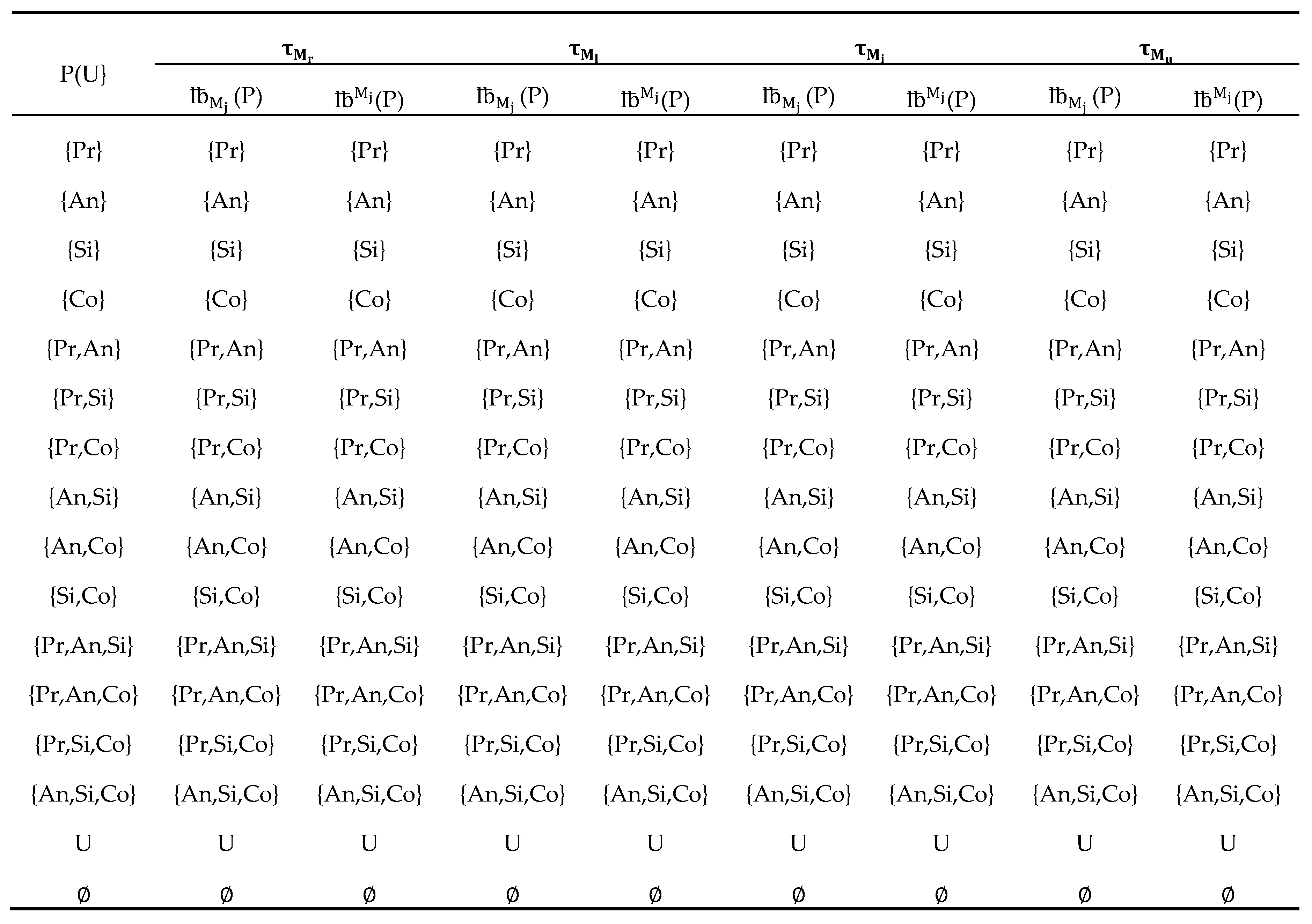
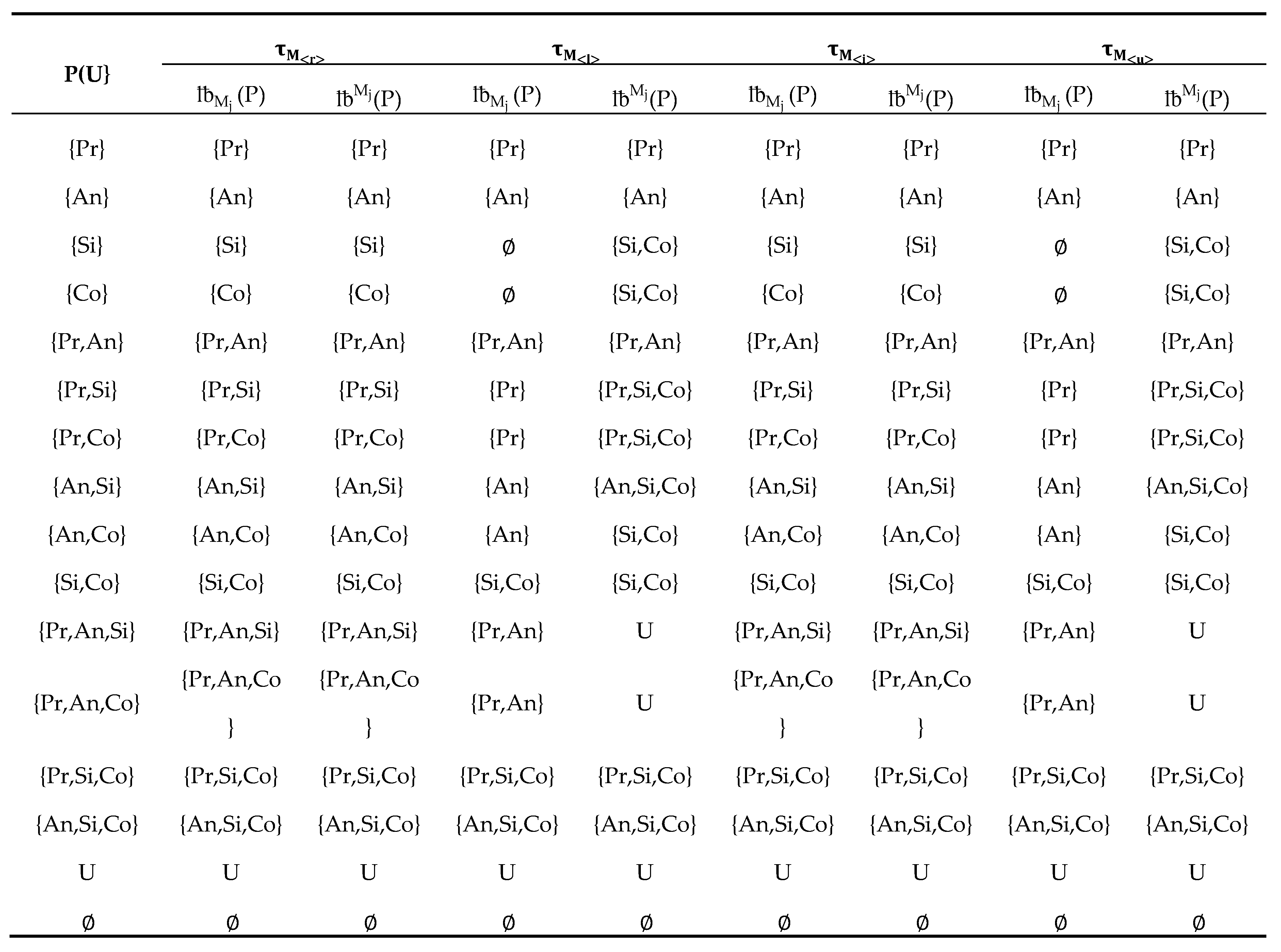
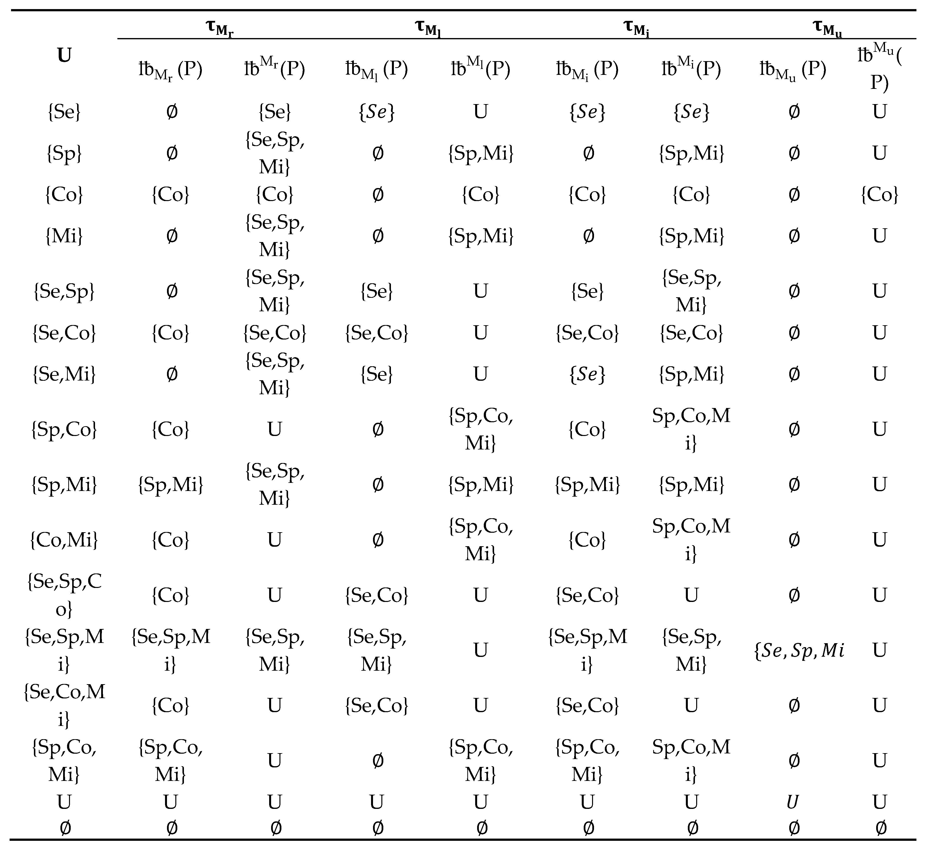
According to the data given in Example 3.1, we get two tables that give

M_{j}

-lower approximations and

M_{j}

- upper approximations for

j \in {r, l, i, u}

as shown in Table 4 and for

j \in {‹ r ›, ‹ l ›, ‹ i ›, ‹ u ›

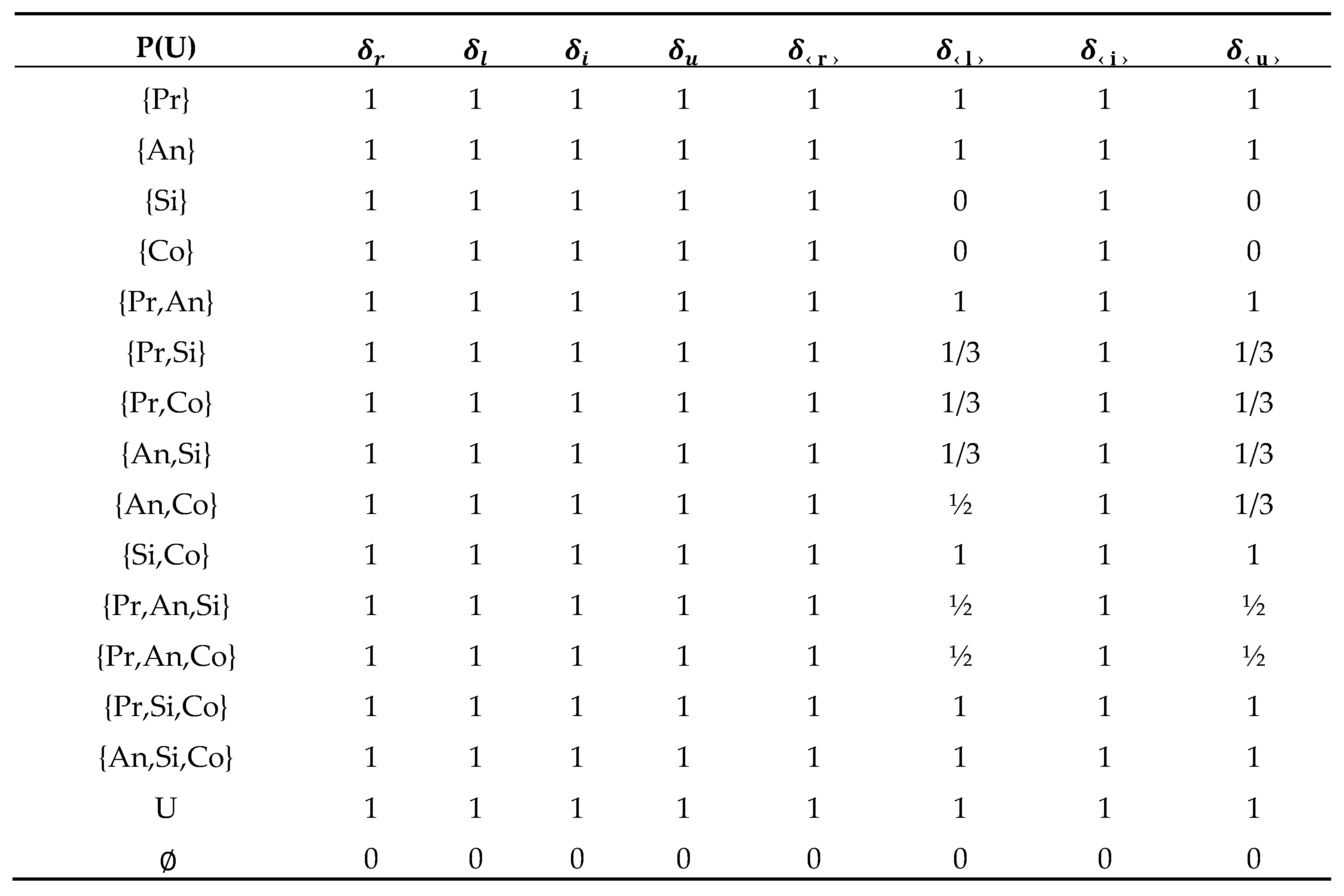
}as shown in Table 5. The

M_{j}

-accuracy for

j \in {r, l, i, u, ‹ r ›, ‹ l ›, ‹ i ›, ‹ u ›}

as shown in Table 6.

9. Comparison between our approach and previous approaches.

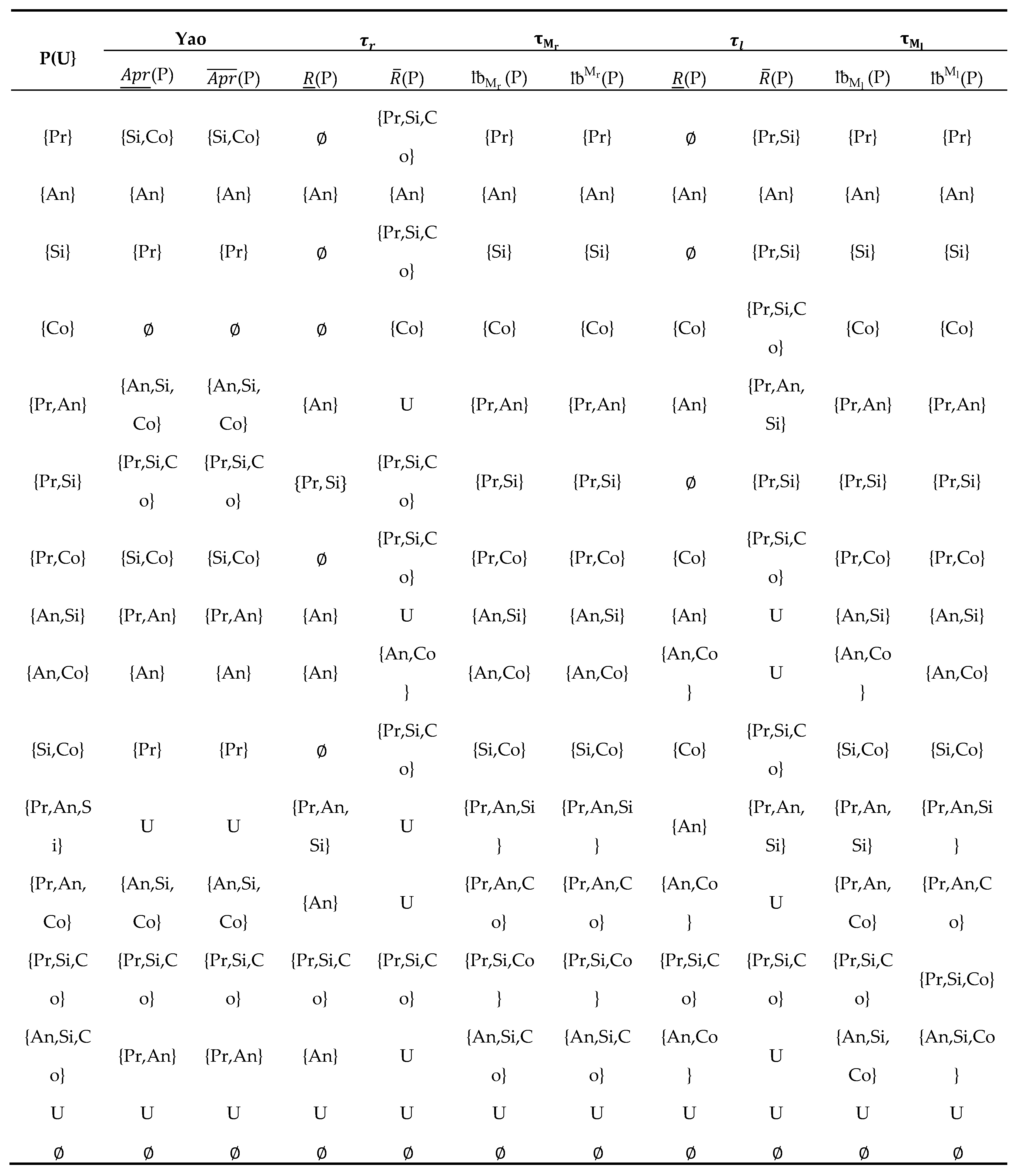
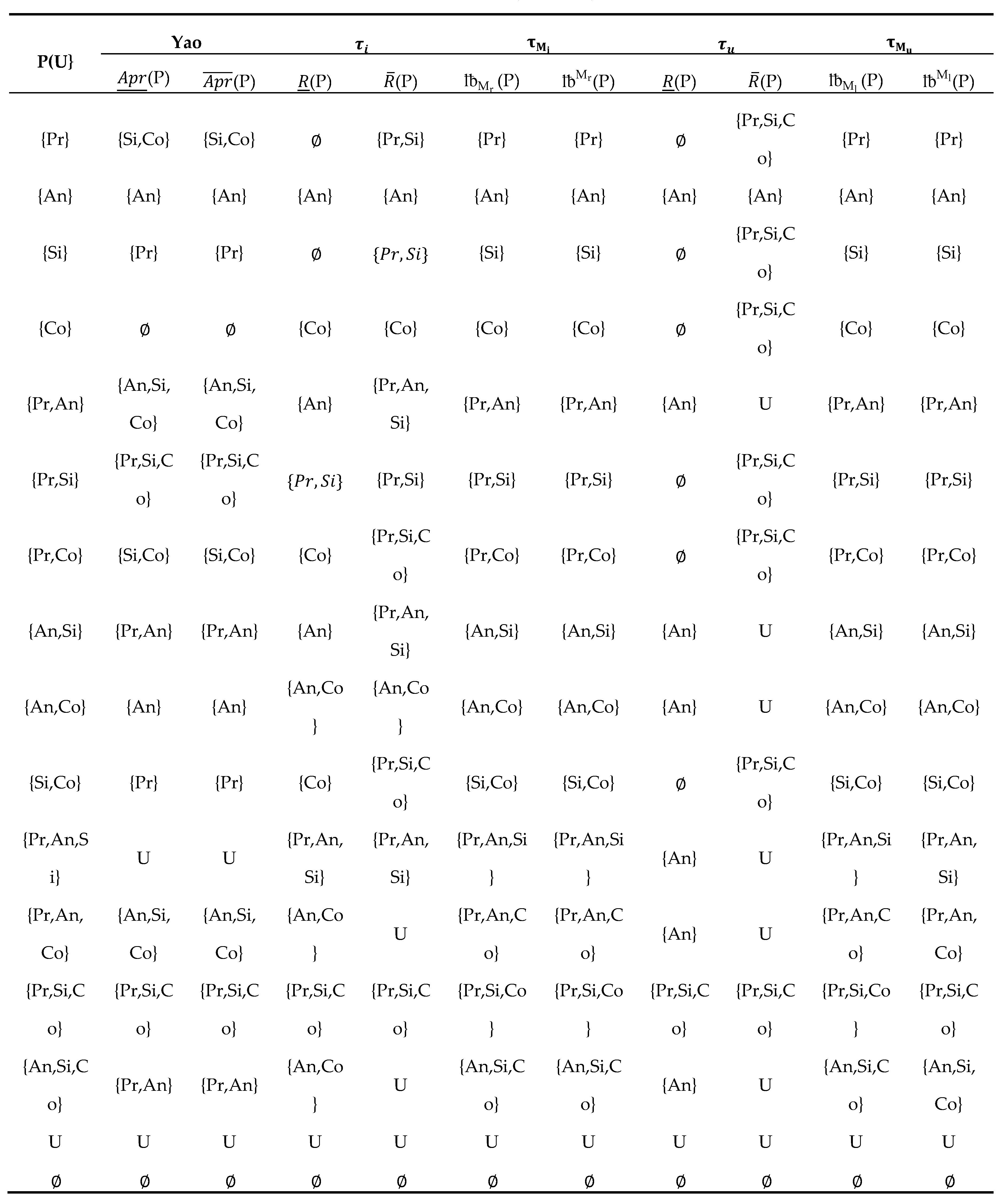
According to data given in Example 3.1. Table 7 and Table 8 provide a comparison between Yao’s method [21], Abd El-Monsef et al.’s method [12]

(τ_{j})

, and the current methods

(τ_{M_{j})}

in case of

j = r, l, i and u,

respectively.

From the Table 7 and Table 8, it is clear that the best of these methods given by using

τ_{M_{r}}, τ_{M_{l}}, τ_{M_{i}}, τ_{M_{〈 r 〉}}, τ_{M_{〈 i 〉}} .

The boundary regions, in this case, are canceled. The results are so important for eliminating the imprecision of rough sets.

Example 9.1. We give the following example to illuminate some consequences.

Suppose that our universe is a set of cars

U = {S e d a n (S e), S p o r t s C a r (S p), C o u p e (C o), M i n i v a n (M i)}

and our relationship is given as

Q = {(S e, S e), (M i, M i), (S e, C o), (S e, M i), (M i, S p), (S p, M i)}

. The different types of neighborhoods are given inTable 9as follows:

The

M_{j}

-Topologies as follows:

τ_{M_{r} =} {U, φ, {Co}, {Sp, Mi}, {Sp, Co, Mi}, {Se, Sp, Mi}} .

τ_{M_{l} =} {U, φ, {Se}, {Se, Co}, {Se, Sp, Mi}} .

τ_{M_{i} =} {U, φ, {Se}, {Co}, {Sp, Mi}, {Se, Co}, {Se, Sp, Mi}, {Sp, Co, Mi}}

τ_{M_{u} =} {U, φ, {Se, Sp, Mi}} .

τ_{M_{‹ r ›} =} {U, φ, {Mi}, {Sp, Mi}, {Se, Co, Mi}}

τ_{M_{‹ l ›} =} {U, φ, {Se}, {Co}, {Mi}, {Se, Co}, {Se, Mi}, {Co, Mi}, {Se, Sp, Mi}, {Se, Co, Mi}}

τ_{M_{‹ i ›} =} {\begin{matrix} U, φ, {Co}, {Se}, {Mi}, {Se, Co}, {Sp, Mi}, {Se, Mi}, \\ {Co, Mi}, {Se, Sp, Mi}, {Se, Co, Mi}, {S p, C o, M i} \end{matrix}} .

τ_{M_{‹ u ›} =} {U, φ, {Mi}, {Se, Co, Mi}} .

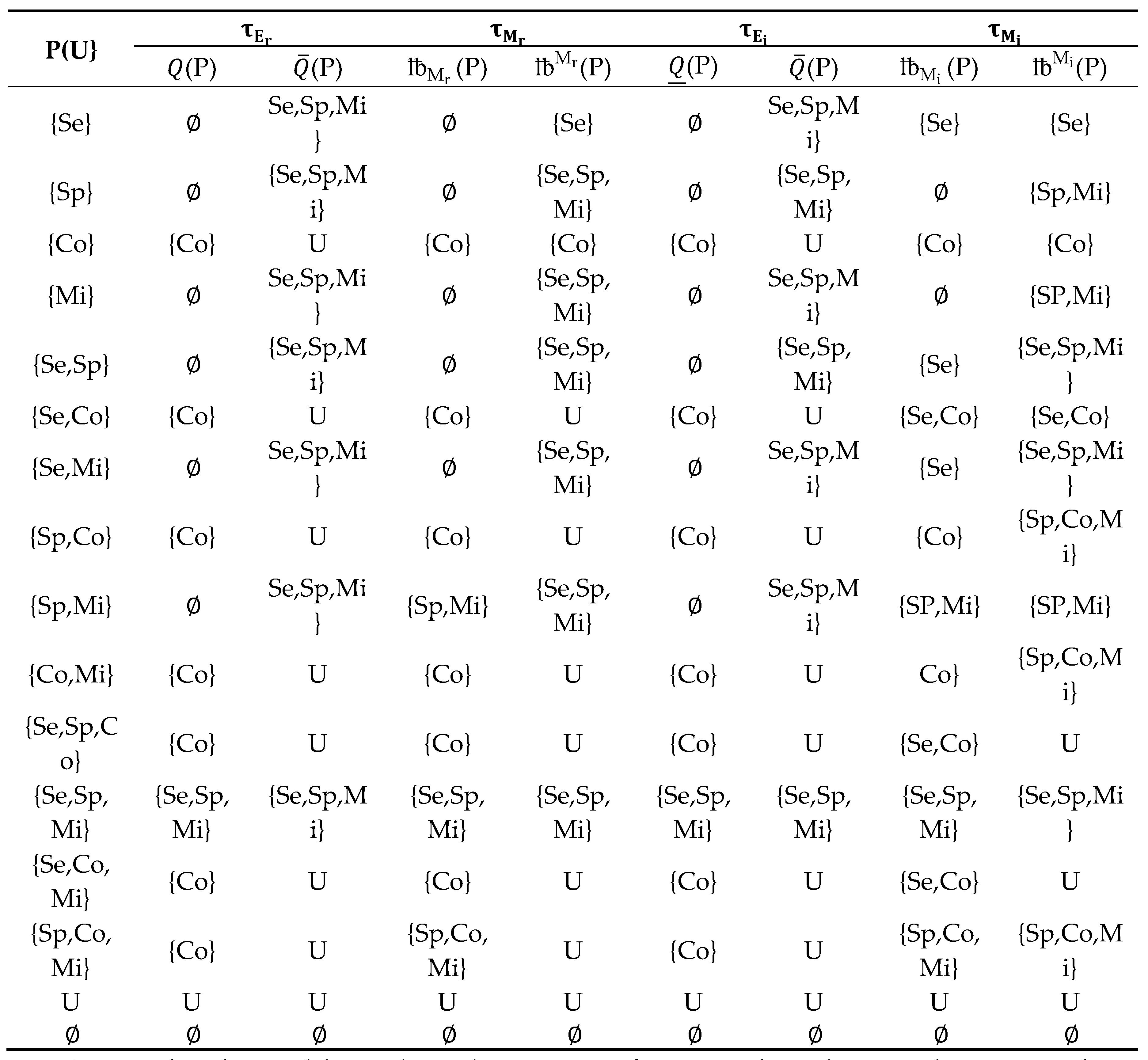
Table 10 give

M_{j}

-lower approximations and

M_{j}

- upper approximations for each

j \in {r, l, i, u}

. Table 11 shows the comparison between Tareq M. Al-shami [18]

(τ_{E_{j})}

approach and

the current

approach

(τ_{M_{j}})

in case of j

\in

{r,i} as given in Example 9.1. The

M_{j}

-accuracy for each

j \in {r, l, i, u}

are given in

We complete this work by studying these concepts from a topological view and comparing them. In all comparisons, we obtain higher accurate approximations in our approach.

10. Conclusions

This paper generated some classes of neighborhood systems that we call them

M_{j}

-neighborhoods. We introduced some examples to discuss the main structures and their main concepts. We generalized these concepts to the topological case. We addressed many possible comparisons among them. We obtained refinement results that can be useful in real-life applications.

Author Contributions

Conceptualization, A.S. Salama and M. S. Bondok.; methodology, A.S. Salama.; software, A. A. El Atik and O.A. Embaby.; validation, A.S. Salama and M.S. Bondok.; formal analysis, A.M. Hussein.; investigation, A.S. Salama.; resources, A.S. Salama and M. S. Bondok.; data curation, M.S. Bondok; writing—original draft preparation, A.S. Salama.; writing—review and editing, A.S. Salama.; visualization, A. A. El Atik and O.A. Embaby; supervision, A.S. Salama; project administration, A.M.Hussein; funding acquisition. All authors have read and agreed to the published version of the manuscript.

Funding

This research received no external funding.

Data Availability Statement

MDPI Research Data Policies at https://www.mdpi.com/ethics.

Acknowledgments

The author sincerely thank the editor and to anonymous reviewers for their valuable comments and suggestions that helped in improving this paper. The authors would like to thank all Tanta Topological Seminar colleagues ‘‘under the leadership of Prof. Dr. A. M. Kozae’’ for their interests.

Conflicts of Interest

The authors declare no conflict of interest.

References

Z. Pawlak, Rough sets, Int. J. Inf. Comput. Sci. 11 (5) (1982) 341–356.
Z. Pawlak, A. Skowron, Rough sets, Some extensions, Information Sciences, 177 (2007) 28–40.
K. Qin, J. Yang, Z. Pei, Generalized rough sets based on reflexive and transitive relations, Information Sciences, 178 (2008) 4138–4144.
W. Zhu, F. Wang, Reduction and axiomatization of covering generalized rough sets, Information Sciences, 152 (2003) 217–230.
W. Zhu, F. Wang, Binary relation based rough sets, Lecture Notes in Computer Sciences, 4223 (2006) 276–285.
A. S. Salama, Generalizations of Rough Sets Using two Topological Spaces with Medical Applications, INFORMATION, 19 (7A) (2016) 2425-2440.
A.S. Salama, Sequences of Topological Near Open and Near Closed Sets with Rough Applications, Filomat, 34(1) (2020), 51–58.
A.S. Salama, Bitopological Approximation Space with Application to Data Reduction in Multi-valued Information Systems, Filomat, 34 (1) (2020), 99–110.
A.S. Salama, Topological solution of missing attribute values problem in incomplete information tables, Information Sciences, 180 (2010) 631-639.
A.S. Salama, Topologies induced by relations with applications, Journal of Computer Science, 4(10) (2008), 877–887.
A.S. Salama, Abd El-Monsef, M. M. E., New topological approach of rough set generalizations, International Journal of Computer Mathematics, 88(7) (2011), 1347–1357.
M.E. Abd El-Monsef, O.A. Embaby, M.K. El-Bably, Comparison between rough set approximations based on different topologies, International Journal of Granular Computing, Rough Set and Intelligent Systems, 3(4) (2014), 292–305.
M.E. Abd El-Monsef, A.S. Salama and O.A. Embaby, Granular computing using mixed neighborhood systems, Journal of Institute of Mathematics and Computer Sciences, 20 (2) (2009), 233–243. O.G.
El Barbary, A.S. Salama, Feature selection for document classification based on topology, Egyptian Informatics Journal, 19(2) (2018), 129–132.
Wiweger, On topological rough sets, Bulletin of the Polish Academy of Sciences Mathematics, 37 (1989) 89–93.
Tareq M. Al-shami, An improvement of rough sets’ accuracy measure using containment neighborhoods with a medical application. Inf Sci, 569 (2021),110–124.
Tareq, M. Al-shami, Ciucci D, Subset neighborhood rough sets. Knowl Based Syst, 237 (2022), 107868.
Tareq, M. Al-shami, Fu WQ, Abo-Tabl E. A., New rough approximations based on E-neighborhoods. Complexity, 6666853 (2021), 1-6.
Mareay R, Generalized rough sets based on neighborhood systems and topological spaces, Journal of Egyptian Math Soc, 24 (2016) 603–608.
Z. Pawlak, Rough Sets, Theoretical Aspects of Reasoning About Data, Kluwer Acadmic Publishers Dordrecht, 1991.
Yao YY, Two views of the theory of rough sets in finite universes. Int J Approx Reason, (1996), 15:291–317.

Table 1. Classes of

N_{j}

-neighborhoods, E_j-neighborhoods and M_j -neighborhoods.

Table 1. Classes of

N_{j}

-neighborhoods, E_j-neighborhoods and M_j -neighborhoods.

Table 2. The approximations and accuracy measure in cases of

j \in {r, l, I, u} .

Table 2. The approximations and accuracy measure in cases of

j \in {r, l, I, u} .

Table 3. The approximations and accuracy measure in cases of

j \in {‹ r ›, ‹ l ›, ‹ i ›, ‹ u ›}

Table 3. The approximations and accuracy measure in cases of

j \in {‹ r ›, ‹ l ›, ‹ i ›, ‹ u ›}

Table 4. The

M_{j}

-approximations for each

j \in {r, l, i, u}

Table 4. The

M_{j}

-approximations for each

j \in {r, l, i, u}

Table 5. The

M_{j}

-approximations for each

j \in {‹ r ›, ‹ l ›, ‹ i ›, ‹ u ›}

Table 5. The

M_{j}

-approximations for each

j \in {‹ r ›, ‹ l ›, ‹ i ›, ‹ u ›}

Table 6. The

M_{j}

-accuracy for

j \in {r, l, i, u, ‹ r ›, ‹ l ›, ‹ i ›, ‹ u ›}

Table 6. The

M_{j}

-accuracy for

j \in {r, l, i, u, ‹ r ›, ‹ l ›, ‹ i ›, ‹ u ›}

Table 7. Comparison between Yao,

τ_{j}

and M_j approaches for j = (r, l).

Table 7. Comparison between Yao,

τ_{j}

and M_j approaches for j = (r, l).

Table 8. Comparison between Yao,

τ_{j}

and M_j approaches for j = (r, l).

Table 8. Comparison between Yao,

τ_{j}

and M_j approaches for j = (r, l).

Table 9. Different types of neighborhoods.

U	Sedan	Sports Car	Coupe	Minivan
$N_{r}$	{Se,Co,Mi}	{Mi}	$\emptyset$	{Sp,Mi}
$N_{l}$	{Se}	{Mi}	{Se}	{Se,Sp,Mi}
$N_{i}$	{Se}	{Mi}	$\emptyset$	{Sp,Mi}
$N_{u}$	{Se,Co,Mi}	{Mi}	{Se}	{Se,Sp,Mi}
$N_{‹ r ›}$	{Se,Co,Mi}	{Sp,Mi}	{Se,Co,Mi}	{Mi}
$N_{‹ l ›}$	{Se}	{Se,Sp,Mi}	$\emptyset$	{Mi}
$N_{‹ i ›}$	{Se}	{Sp,Mi}	$\emptyset$	{Mi}
$N_{‹ u ›}$	{Se,Co,Mi}	{Se,Sp,Mi}	{Se,Co,Mi}	{Mi}
$E_{r}$	{Se,Sp,Mi}	{Se,Sp,Mi}	$\emptyset$	{Se,Sp,Mi}
$E_{l}$	{Se,Co,Mi}	{Sp,Mi}	{Se,Co,Mi}	U
$E_{i}$	{Se,Mi}	{Sp,Mi}	$\emptyset$	{Se,Sp,Mi}
$E_{u}$	U	{Se,Sp,Mi}	{Se,Co,Mi}	U
$E_{‹ r ›}$	U	U	U	U
$E_{‹ l ›}$	{Se,Sp}	{Se,Sp,Mi}	$\emptyset$	{Sp,Mi}
$E_{‹ i ›}$	{Se,Sp}	{Se,Sp,Mi}	$\emptyset$	{Sp,Mi}
$E_{‹ u ›}$	U	U	U	U
$M_{r}$	{Se,Mi}	{Mi}	$\emptyset$	{Sp,Mi}
$M_{l}$	{Se}	{Mi}	{Se}	{Se,Sp,Mi}
$M_{i}$	{Se}	{Mi}	$\emptyset$	{Sp,Mi}
$M_{u}$	{Se,Mi}	{Mi}	{Se}	{Se,Sp,Mi}
$M_{‹ r ›}$	{Se,Co,Mi}	{Sp,Mi}	{Se,Co,Mi}	{Mi}
$M_{‹ l ›}$	{Se}	{Se,Sp,Mi}	$\emptyset$	{Mi}
$M_{‹ i ›}$	{Se}	{Sp,Mi}	$\emptyset$	{Mi}
$M_{‹ u ›}$	{Se,Co,Mi}	{Se,Sp,Mi}	{Se,Co,Mi}	{Mi}

Table 10. Approximations operators based on

τ_{M_{j}}

for some subsets of U.

Table 10. Approximations operators based on

τ_{M_{j}}

for some subsets of U.

Table 11. Comparison among

E_{i}

and M_i approaches for some subsets of U.

Table 11. Comparison among

E_{i}

and M_i approaches for some subsets of U.

Disclaimer/Publisher’s Note: The statements, opinions and data contained in all publications are solely those of the individual author(s) and contributor(s) and not of MDPI and/or the editor(s). MDPI and/or the editor(s) disclaim responsibility for any injury to people or property resulting from any ideas, methods, instructions or products referred to in the content.

© 2023 by the authors. Licensee MDPI, Basel, Switzerland. This article is an open access article distributed under the terms and conditions of the Creative Commons Attribution (CC BY) license (http://creativecommons.org/licenses/by/4.0/).

Copyright: This open access article is published under a Creative Commons CC BY 4.0 license, which permit the free download, distribution, and reuse, provided that the author and preprint are cited in any reuse.

Alerts

MDPI Initiatives

Important Links

Choose an area of interest and we will send you notifications of new preprints at your preferred frequency.

Disclaimer

Generalized Rough Neighborhood Approximations and Related Topological Approaches

Abstract

Keywords:

Subject:

1. Introduction

2. Preliminaries

2.1. Pawlak Approximation Space

4. The Relationships Among M j –neighborhoods

5. Generalized Rough Approximations Based on M j –neighborhoods

7. The Relations Among τ M j Topologies

8. Rough Approximations Generated by M j -Topologies

9. Comparison between our approach and previous approaches.

10. Conclusions

Author Contributions

Funding

Data Availability Statement

Acknowledgments

Conflicts of Interest

References

MDPI Initiatives

Important Links

Subscribe

4. The Relationships Among $M_{j}$ –neighborhoods

5. Generalized Rough Approximations Based on $M_{j}$ –neighborhoods

7. The Relations Among $τ_{M_{j}}$ Topologies

8. Rough Approximations Generated by $M_{j}$ -Topologies