1. Introduction
The shortest path problem is a well-established and important problem that finds applications in various fields, including robotics ([
1,
2]), VLSI design ([
3]), wireless sensor networks ([
4]), and transportation ([
5,
6]). This problem can be represented either on a grid or a more general graph, with different techniques employed for each representation. Grid-based approaches are commonly favored in scenarios like extensive VLSI design, particularly when there are numerous obstacles to navigate around.
Traditionally, two types of methods have been used to address the global path planning problem. The first type is exhaustive search, which involves thorough exploration of the entire search space to find the optimal solution. Examples of exact search algorithms commonly used for this purpose include Dijkstra’s algorithm (([
7,
8])) and
algorithm ([
9]). These algorithms guarantee finding the shortest path but may become impractical when dealing with large grids due to their computational complexity.
The second type is local search, which employs metaheuristic algorithms to explore only a portion of the search space. These algorithms, such as Tabu Search ([
10]), Ant Colony Optimization ([
11]), Genetic Algorithm ([
12]), Particle Swarm Optimization ([
13,
14]), and their multiple variants, provide approximate solutions and are often used when the exhaustive search is not feasible due to the large size of the grid. By exploring a limited subset of the search space, local search algorithms can find reasonably good solutions efficiently.
Recently, some relaxed alternatives of exhaustive search algorithms have emerged. These approaches aim to find a balance between the constraint of achieving optimality in path length and the need for faster search times. The work being discussed here falls into this category. It is demonstrated that the proposed Enhanced Relaxed
(
) algorithm is theoretically equivalent to the relaxed
(
,
15]) algorithm in terms of the path length of the solutions it provides. However, it achieves significant savings in terms of time and memory requirements by employing a completely different computation strategy.
By relaxing the constraint of path length optimality to some extent, this approach manages to expedite the search process while still delivering solutions that are comparable in terms of path length to those obtained through the algorithm. The key advantage lies in the adoption of a novel computation strategy based on lookup matrices. These matrices store precomputed values that can be efficiently accessed during the search, eliminating the need for redundant calculations and resulting in substantial time and memory savings.
The remaining of this paper is organized as follows:
Section 2 discussed the most relevant related works.
Section 3 presents the proposed
algorithm and proves its equivalence to
in terms of path cost.
Section 4 presents the results of the evaluation of
on a benchmark of representative grid maps, and compares it to
and
in terms of path cost and execution time. Finally,
Section 5 concludes the paper and suggests some future works.
2. Related Works
Shortest path algorithms are a crucial tool in the field of computer science and are used to solve a wide range of problems. In general, point-to-point shortest path algorithms work by starting at a source node and exploring the neighboring nodes until they reach the destination node. Along the way, the algorithm keeps track of the shortest distance from the source to each node, using this information to guide the search and ensure that the shortest path is found. There are a variety of shortest path algorithms that have been developed for finding the shortest path between two points in a regular grid ([
16]). These algorithms typically involve searching through the grid to identify the optimal path, taking into account factors such as the cost of moving from one cell to another and any obstacles that may be present in the grid.
One of the most popular and well-known shortest path algorithms for regular grids is Dijkstra’s algorithm, which was first proposed by Dutch computer scientist Edsger Dijkstra ([
7,
8]). Dijkstra’s algorithm is a general-purpose algorithm that can be used to find the shortest path between any two points in a weighted, directed graph. It is based on the idea of building a "shortest path tree" from the source point to all other points in the grid, with the shortest path to each point being the minimum sum of the weights of the edges along the path. Although Dijkstra’s algorithm is relatively simple and easy to implement, it has a time complexity of O(
) when using a suitable data structure (Fibonacci heaps), where
is the number of edges in the graph and
is the number of vertices. This makes it less efficient for larger grids.
Another popular shortest path algorithm for regular grids is
[
9], which was proposed as an improvement of Dijkstra’s algorithm.
is a heuristic search algorithm that uses a combination of a best-first search and a cost-estimation function to guide the search towards the goal. Unlike Dijkstra’s algorithm, which considers all paths from the source to the goal,
only considers paths that are likely to lead to the goal, based on the cost-estimation function. This makes
more efficient than Dijkstra’s algorithm for many grid-based problems, although the performance of
can be sensitive to the choice of cost-estimation function.
[
17] proposed the first Maze-solving algorithm that is based on target-directed grid propagation and is memory-efficient. It was extensively employed in the field of printed circuit board design for finding wire paths. However, [
18] later revealed that the original claim of the algorithm’s generality regarding the path cost function is incorrect.
More recent shortest path algorithms for regular grids include the Jump Point Search (JPS) algorithm, proposed by [
19] as an improvement over
in grid maps. It is based on a selective node expanding process that specifically identifies and expands certain nodes in the grid map, referred to as jump points. Thus, intermediate nodes along a path between two jump points are not expanded at all, which enhances the speed of
search by an order of magnitude.
[
20] proposed the Minimum Detour (MD) algorithm in G4 regular grids. Its main idea is to calculate the detour number d(P), defined as the number of nodes on the path P that are directed away from the goal. Then, the path length is calculated as M(S,G) + 2d(P), where M(S,G) is the Manhattan distance between the start S and the goal G nodes. This is because any move opposed to the direction of the goal necessarily needs to be compensated to reach the goal. Since M(S,G) is constant for a given (S,G) pair, minimizing the path length is equivalent to minimizing the detour number. Nodes that have lower detour numbers are given higher priority in the grid expansion process, in a breath-first search style. Since then, no similar algorithm has been proposed in G8 grids, because the detour computation is not as simple as in G4 grids. This paper proposes to bridge this gap by introducing a Hadlock-inspired algorithm applicable to G8 grids.
Relaxed Dijkstra and Relaxed
(
) algorithms proposed by [
15] exploit the grid-map structure to establish an accurate approximation of the optimal path, without visiting any cell more than once. The path length is approximated in terms of number of moves on the grid. This approach distinguishes itself from previous bounded relaxation algorithms of
([
21,
22,
23,
24]) primarily by performing relaxation on the exact cost, denoted as g, of the evaluation function f (where f = g + h). This sets it apart from existing relaxations of the
algorithm, which typically focus on relaxing the heuristic h. The current work proposes aims to further accelerate the execution of the
algorithm by completely changing its computing paradigm, drawing inspiration from the Hadlock algorithm.
It is worth noting that path planning in a grid map can be substantially accelerated in a completely different way by building connection graphs before applying a search algorithm ([
25]). Nevertheless, the fact that the proposed
algorithm does not construct connection graphs is a significant advantage in many cases. For instance, in large VLSI design problems with a high number of obstacles, the construction of the entire connection graph could be extremely costly.
3. Methodology
The proposed algorithm is based on calculating detour penalties that are propagated from the source node S to the the goal node G. For a given current node C, we define:
: the angle between the x-axis and the vector.
, where and are the abscissas of the goal node and the current node, respectively.
, where and are the ordinates of the goal node and the current node, respectively.
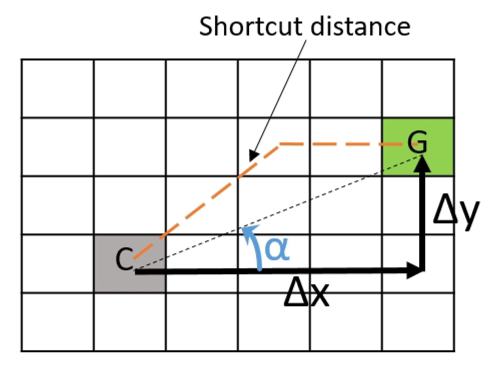
Figure 1 clarifies the definition of the variables
,
, and
on an example.
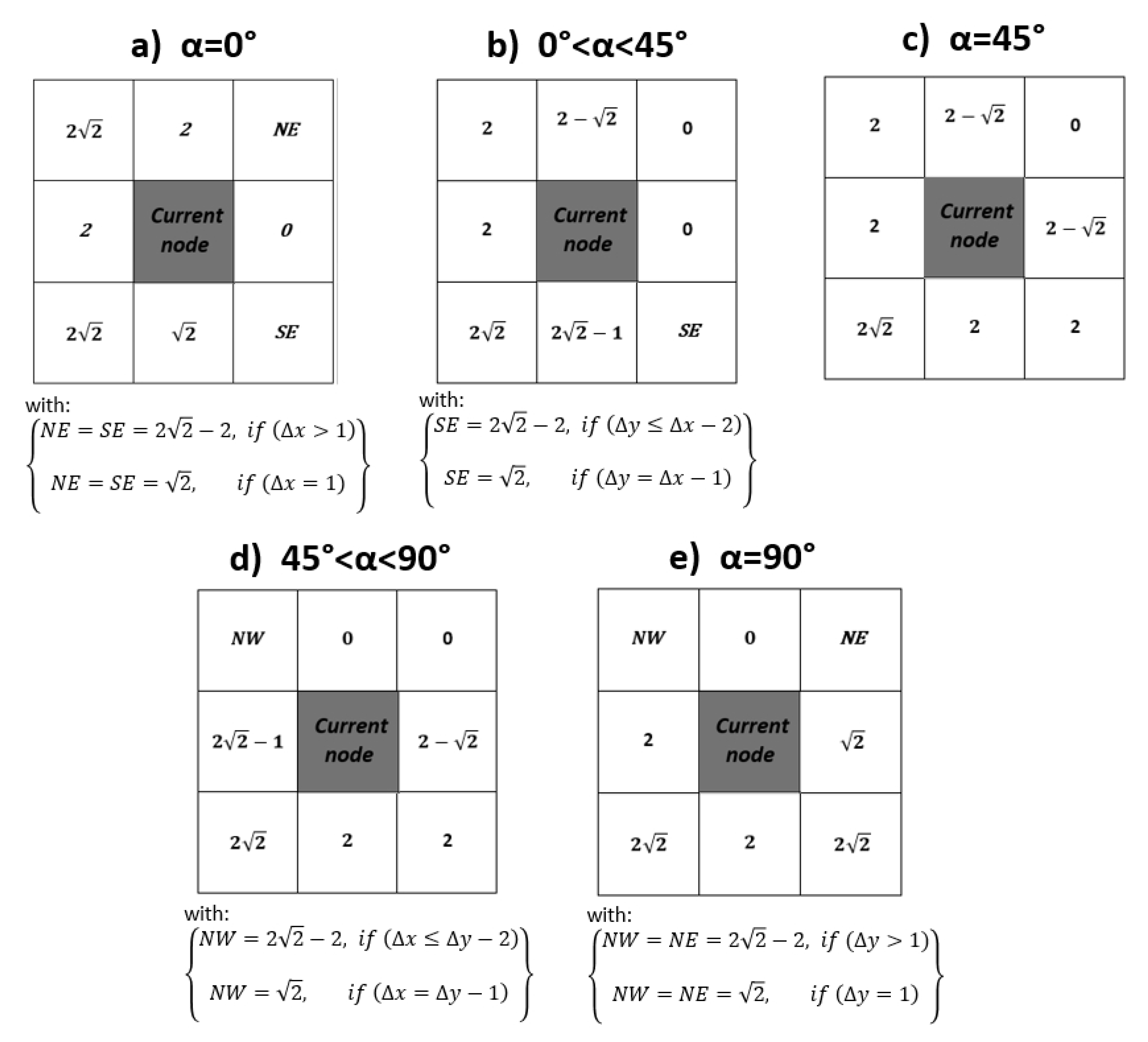
Figure 2 presents the five first matrices of incremental detour penalty for
. These 3x3 matrices store the incremental detour (penalty) from the goal expressed as:
Where
h is the shortcut distance to goal (shortest path assuming there are no obstacles, see
Figure 1).
The value of some penalties, which are denoted as NE (North-East), SE (South-East), and NW (North-West), depend on the value of and . For instance, in case (a), corresponding to (C and G on the same row, with G on the right, so that the optimal path between them is equal to ), if , it means that the goal is adjacent to the current node on its right. Consequently, if we move towards NE or SE, we will reach the goal with a minimum cost of instead of just 1 for the optimal path between C and G. That is why the penalty is . Whereas, for all other values of , if we move towards NE, we can return back to the row containing G with a total cost of instead of 2 for the optimal path. That is why the penalty is . Obviously, the case cannot correspond to angle . The reasoning is similar for the other cases.
Notice that the matrix (e) can be obtained from the matrix (a) by applying a 90° anti-clockwise rotation and substituting for in the formulas of NE/SE that becomes NW/NE. Likewise:
(f) : is obtained from (b) by applying a 90° anti-clockwise rotation.
(g) : is obtained from (c) by applying a 90° anti-clockwise rotation.
(h) : is obtained from (d) by applying a 90° anti-clockwise rotation.
In total, we have 28 fixed matrices (counting the cases of different and values), that we store before running the search algorithm.
As in [
20], nodes that have lower detour numbers are given higher priority in the grid expansion process. This process proceeds until the goal position is reached. Then the path is reconstructed backwards from the goal cell, by moving from each cell to its parent cell that expanded it, until the starting cell is reached.
Instead of two matrices (actual cost
g and combined score
f) as in
and
, only one matrix of detour penalties (
D) is stored in memory. At a give node
, the detour value can be calculated recursively, using the euclidean distance
and the heuristic function
h (shortcut distance), as:
Consequently, since is constant, optimizing D is equivalent to optimizing f.
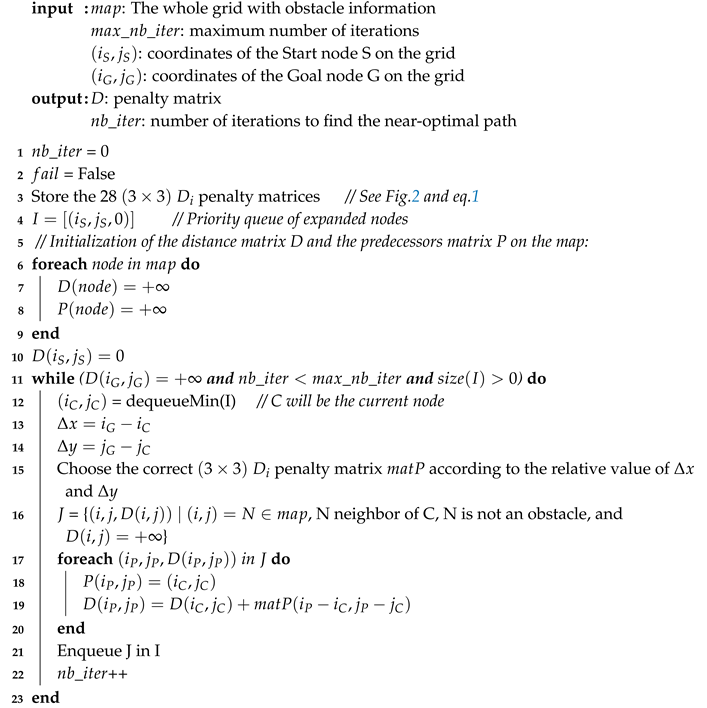
Algorithm 1 presents the main steps for path exploration in
. The algorithm takes as input a grid represented by a 2D matrix (
) where obstacles are marked with a predefined value, and the coordinates of the start (S) and goal (G) nodes. It calculates the penalty matrix D with a finite value for all explored nodes. The algorithm stops when the node exploration reaches G, or when a predefined maximum number of iterations is reached. We first store the 28
incremental penalty matrices (see
Figure 2), and initialize the priority queue I of expanded nodes to the start node S with associated penalty 0 (line 4). The penalty matrix D and the Predecessor matrix P (used for path reconstruction) are both initialized with default infinity values (lines 6-8), except for the penalty associated with S which is initialized to 0 (line 10). Then, we iterate over the priority queue I by dequeuing each time the node that has the minimum penalty value
. Based on the value of
and
between this current node C and the goal node, we choose the corresponding incremental penalty matrix
. This choice is accomplished through a series of if statements where the most likely cases (e.g., inequalities such as
) are placed before less likely cases (e.g., equalities such as
), in order to optimize execution time. We define J (line 16) as the set of all free (i.e., non-obstacle) neighbor nodes of C for which the penalty value
is infinite (i.e., has not been calculated yet). For each node in J, we save its predecessor C in the P matrix (line 17) for later path reconstruction, and we calculate its penalty value
as the sum of the current node’s penalty plus the corresponding incremental penalty in the
matrix (line 18). Then, we enqueue J in I (line 21), where the priorities correspond to the D values. If there is a path between S and G, G will be reached and its penalty value calculated, unless the predefined maximum number of iteration is attained.
|
Algorithm 1: search algorithm. |
 |
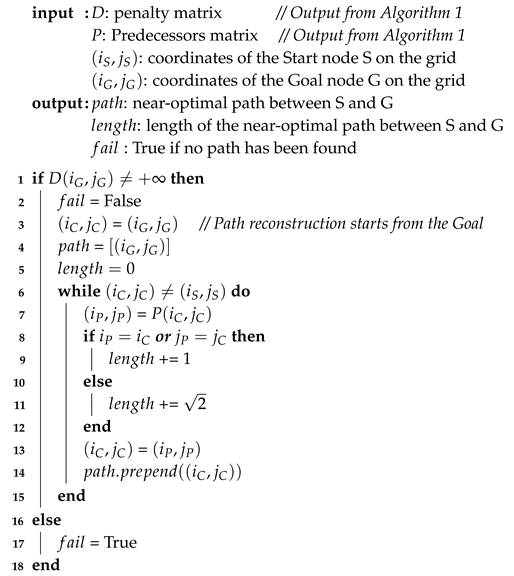
Once Algorithm 1 reaches the goal G, Algorithm 2 is used to reconstruct the path backward. It takes as input the penalty matrix D and predecessors matrix P that were both generated in Algorithm 1, and the start and goal coordinates on the grid. If
(line 1), it means that Algorithm 1 has reached the goal and a path from S to G has been found. The path reconstruction algorithm starts from the goal
(line 3), and prepends the current node’s predecessor to the path at each iteration (line 14), while adding 1 (for horizontal and vertical moves) or
(for diagonal moves) until it reaches the start node S. Alternatively, we can count the number of diagonal moves, and multiply it by
only at the end to avoid accumulating numerical inaccuracies.
|
Algorithm 2: path reconstruction algorithm. |
 |
5. Conclusion
In conclusion, this paper introduced a novel algorithm for solving the point-to-point shortest path problem on a static regular 8-neighbor connectivity (G8) grid. The algorithm is a generalized version of the Hadlock algorithm specifically designed for G8 grids. This work falls within the category of relaxed alternative algorithms that balance the trade-off between path length optimality and search time. By relaxing the constraint of path length optimality to some extent, the proposed Enhanced Relaxed A* (ERA*) algorithm accelerates the search process while still providing solutions with similar path lengths to those obtained using RA*. The key advantage lies in the novel computation strategy utilizing lookup matrices, which significantly reduces redundant calculations, resulting in substantial time and memory savings.
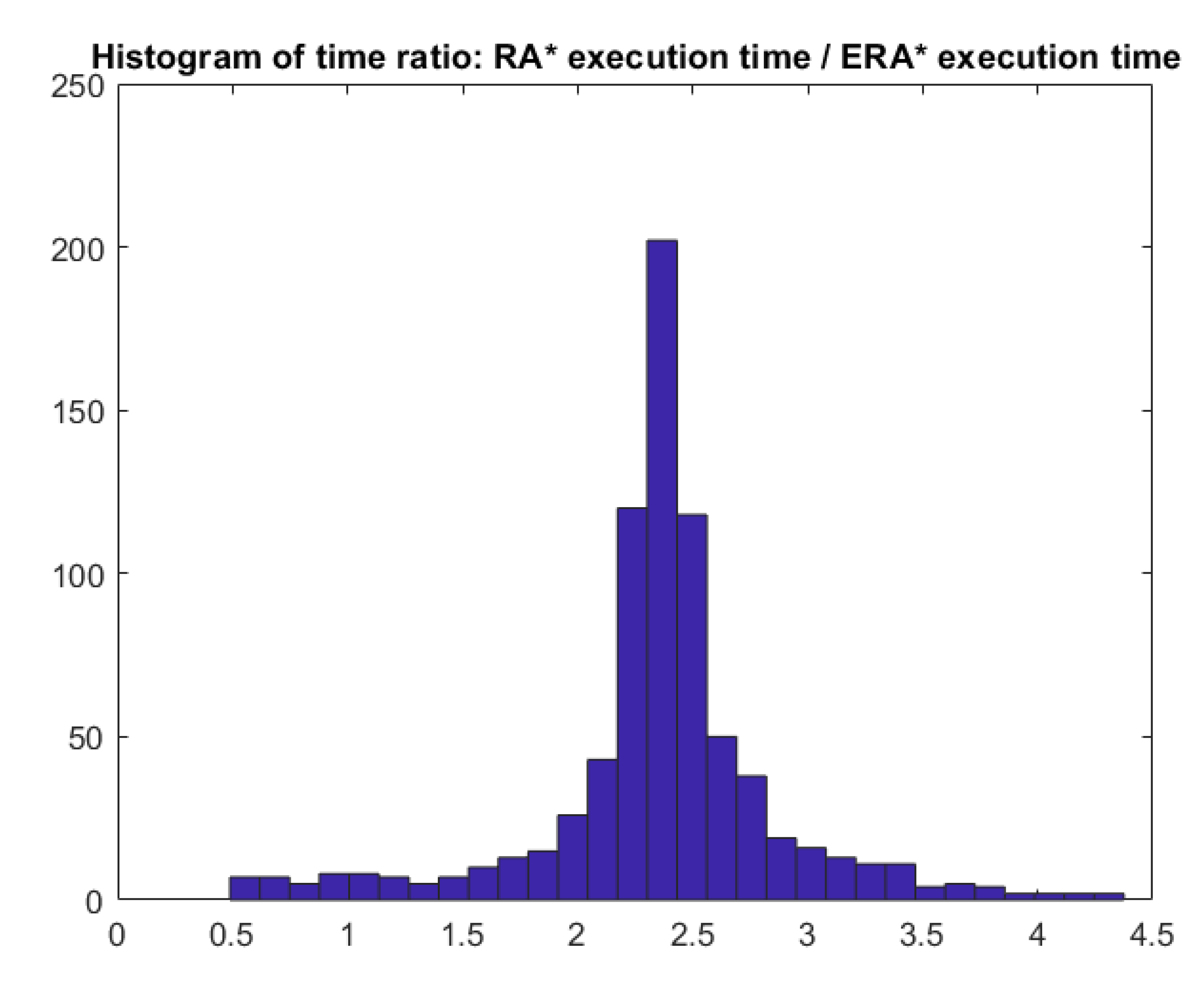
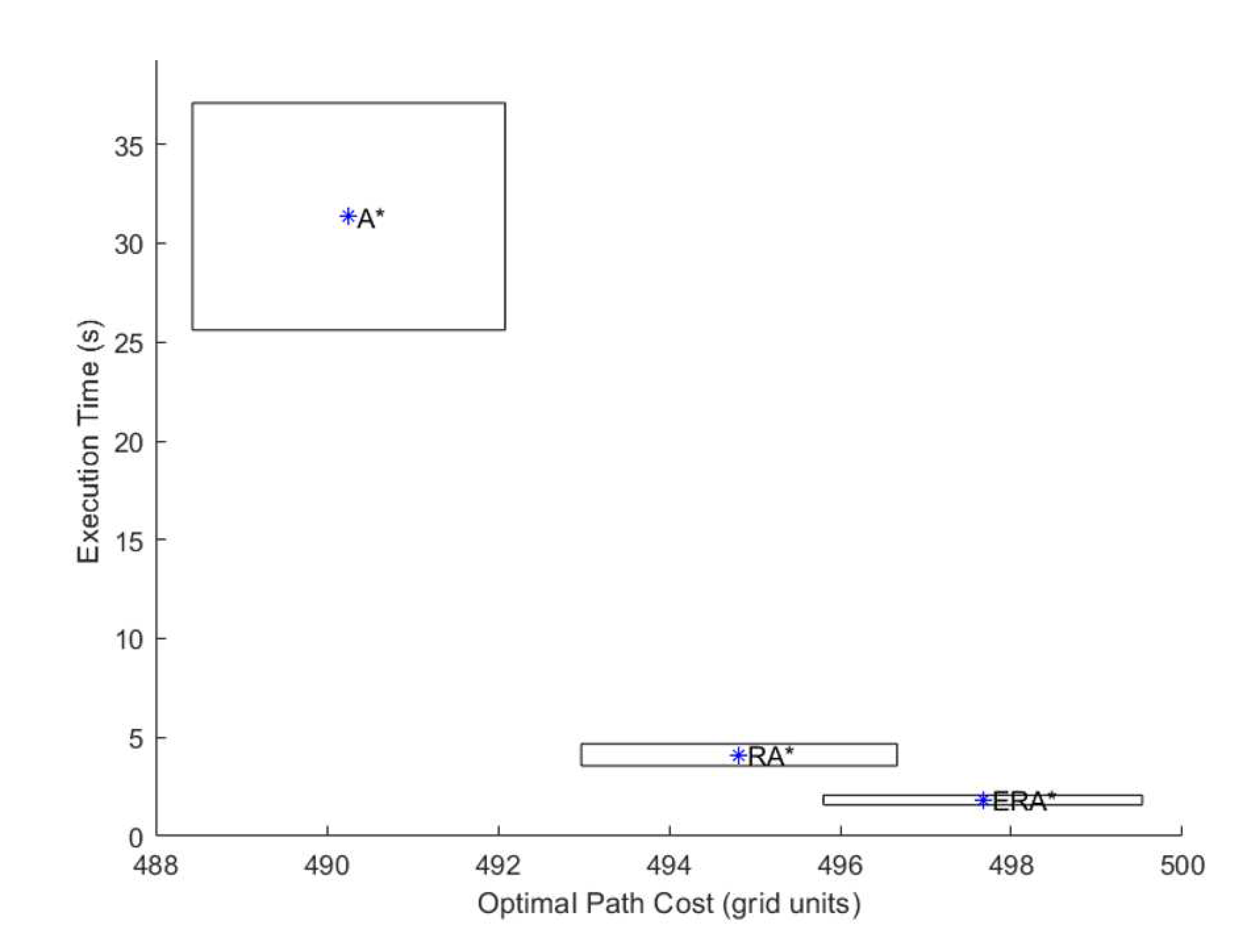
Experimental results obtained through extensive testing on various grid maps validate the algorithm’s effectiveness. On average, it is 2.25 times faster than RA* and 17 times faster than the original A* algorithm. Additionally, it exhibits improved memory efficiency since it eliminates the need for storing a G score matrix.
Future research can focus on exploring further optimizations and extensions of the ERA* algorithm. This could involve investigating its performance in dynamic or uncertain environments, incorporating additional constraints or cost factors, and exploring possibilities for parallelization or distributed computation. Additionally, the algorithm’s applicability to other grid types or graph structures can be explored. The insights gained from this work lay the foundation for potential advancements in efficient path planning algorithms for various domains and applications.
Figure 1.
Example showing the angle α between the current node (C) and the goal node (G), , , and the shortcut distance between C and G, which corresponds to the minimum distance in a G8 grid when there are no obstacles between the two nodes.
Figure 1.
Example showing the angle α between the current node (C) and the goal node (G), , , and the shortcut distance between C and G, which corresponds to the minimum distance in a G8 grid when there are no obstacles between the two nodes.
Figure 2.
Incremental detour penalty lookup matrices for angles between the current node and the goal node from 0° to 90°. The remaining cases can be obtained from the above cases, using simple 90° rotations of the 3x3 matrix. NE, SE, and NW stand for Northeast, Southeast, and Northwest, respectively. These incremental penalties are added when propagating the total penalty the source node to the goal node.
Figure 3.
Histogram of the execution time ratio between and algorithms.
Figure 3.
Histogram of the execution time ratio between and algorithms.
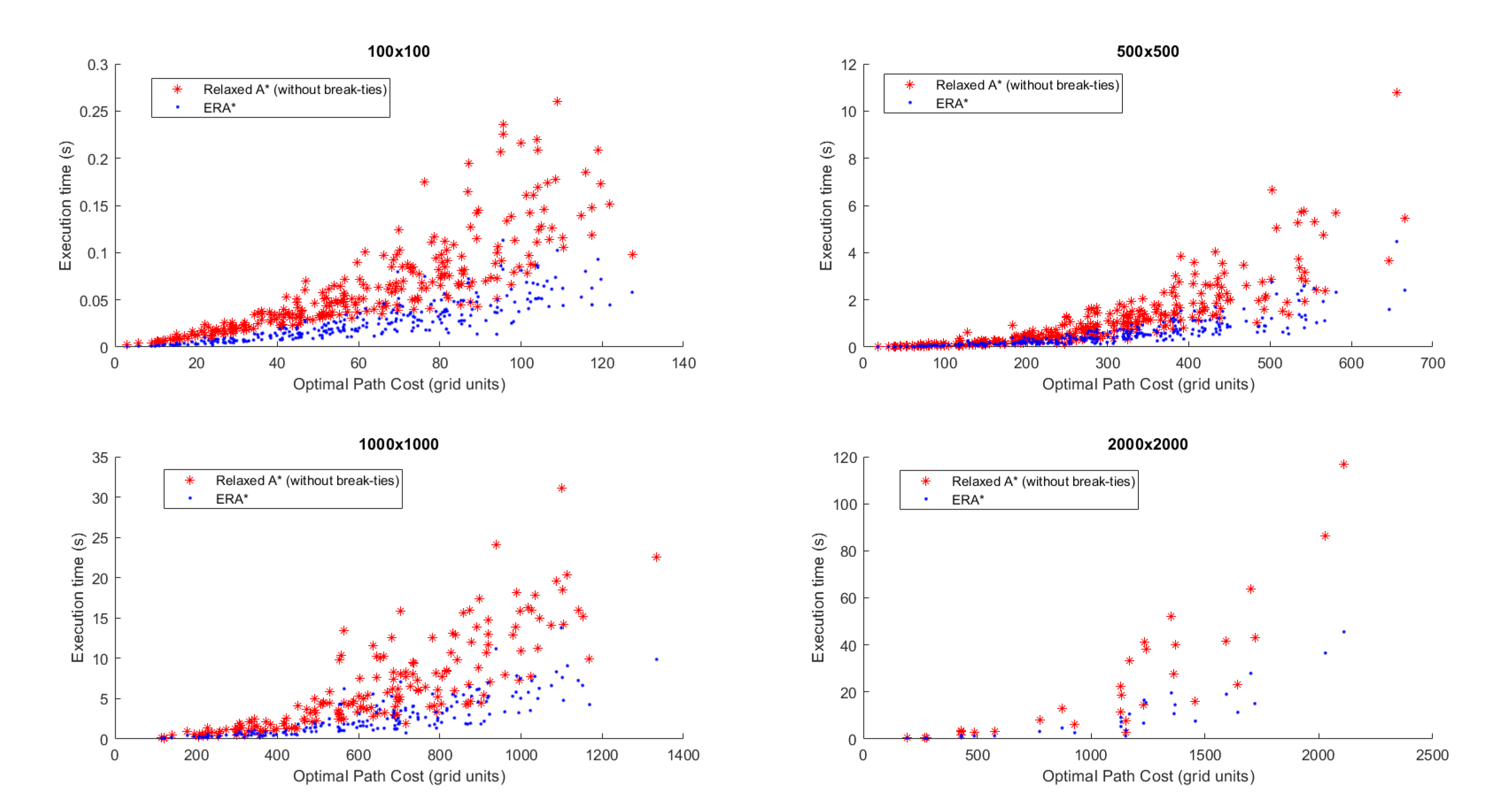
Figure 4.
Comparison of execution time between the proposed (in blue) and (in red) algorithms, for different environment sizes (from 100x100 to 2000x2000 nodes), randomly generated.
Figure 4.
Comparison of execution time between the proposed (in blue) and (in red) algorithms, for different environment sizes (from 100x100 to 2000x2000 nodes), randomly generated.
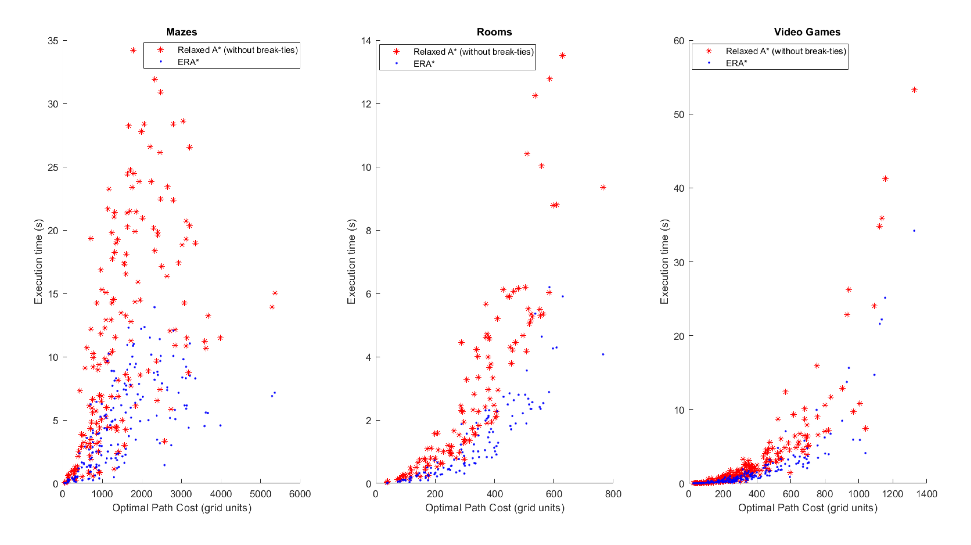
Figure 5.
Comparison of execution time between the proposed (in blue) and (in red) algorithms, for different structured environments.
Figure 5.
Comparison of execution time between the proposed (in blue) and (in red) algorithms, for different structured environments.
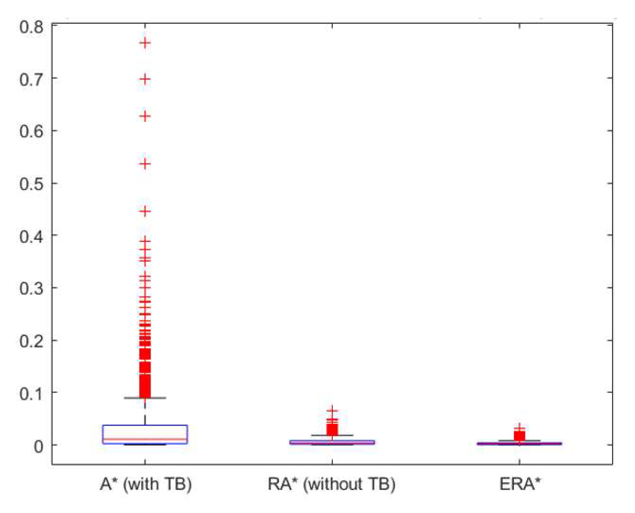
Figure 6.
Box plot of the execution time divided by the optimal path length, for , and algorithms.
Figure 6.
Box plot of the execution time divided by the optimal path length, for , and algorithms.
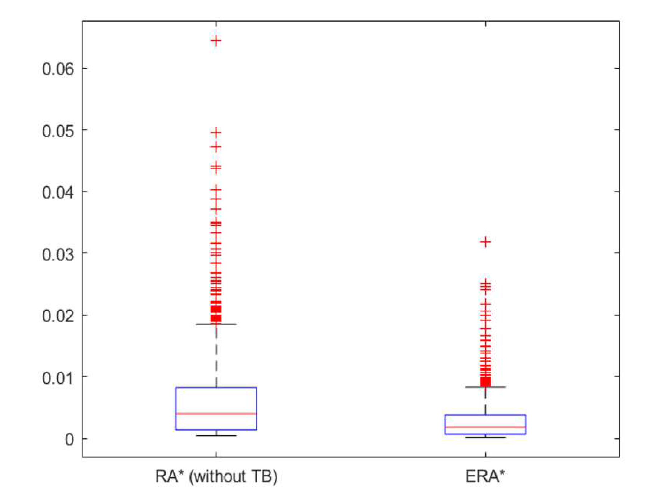
Figure 7.
Box plot of the execution time divided by the optimal path length, for and algorithms.
Figure 7.
Box plot of the execution time divided by the optimal path length, for and algorithms.
Figure 8.
Comparison between the tested algorithms in cost/time space, in terms of average and standard deviation. The width of each rectangle is proportional to the path cost standard deviation, and its height is proportional to the execution time standard deviation. The average is represented by a star at the center of each rectangle.
Table 1.
Percentage of exact optimal paths (when a path exists) per environment, for the three tested algorithms.
Table 1.
Percentage of exact optimal paths (when a path exists) per environment, for the three tested algorithms.
| Algorithm |
100x100 |
500x500 |
1000x1000 |
2000x2000 |
Mazes
(512x512) |
Rooms
(512x512) |
VideoGames
(512x512 to
1024x1024) |
All |
|
100.0% |
100.0% |
100.0% |
100.0% |
100.0% |
100.0% |
100.0% |
100.0% |
|
79.6% |
85.0% |
78.9% |
96.7% |
21.7% |
25.0% |
47.2% |
62.9% |
|
81.9% |
86.0% |
80.6% |
96.7% |
4.4% |
23.3% |
46.7% |
61.1% |
Table 2.
Average path cost per environment size, in cell units.
Table 2.
Average path cost per environment size, in cell units.
| Algorithm |
100x100 |
500x500 |
1000x1000 |
2000x2000 |
Mazes
(512x512) |
Rooms
(512x512) |
VideoGames
(512x512 to
1024x1024) |
All |
|
60.4 |
284.8 |
631.2 |
1086.2 |
1479.1 |
317.1 |
375.8 |
490.3 |
|
60.7 |
285 |
632.3 |
1086.3 |
1501 |
321 |
381.3 |
494.8 |
|
60.7 |
285.2 |
633 |
1086.3 |
1517 |
323.6 |
382.8 |
497.7 |
Table 3.
Percentage of extra length compared to optimal path, calculated for non-optimal paths over all environments.
Table 3.
Percentage of extra length compared to optimal path, calculated for non-optimal paths over all environments.
| Algorithm |
Mean |
Std |
Max |
|
1.7% |
1.6% |
10.7% |
|
2.3% |
1.8% |
10.4% |
Table 4.
Average execution time (in seconds).
Table 4.
Average execution time (in seconds).
| Algorithm |
100x100 |
500x500 |
1000x1000 |
2000x2000 |
Mazes
(512x512) |
Rooms
(512x512) |
VideoGames
(512x512 to
1024x1024) |
All |
|
0.23 |
3.71 |
39.27 |
113.96 |
113 |
17.76 |
29.97 |
31.35 |
|
0.06 |
1.15 |
6.33 |
24.82 |
11.04 |
2.87 |
3.5 |
4.12 |
|
0.03 |
0.51 |
2.71 |
10.05 |
4.65 |
1.3 |
2.01 |
1.83 |
Table 5.
Percentage of runs for which each algorithm appears in rank 1 to 3, with regards to the execution time.
Table 5.
Percentage of runs for which each algorithm appears in rank 1 to 3, with regards to the execution time.
| Rank |
1 |
2 |
3 |
|
9.0% |
5.3% |
85.7% |
|
1.1% |
86.6% |
12.3% |
|
89.9% |
8.1% |
2.0% |
