Identification of Damage in Planar Multi-Storey Reinforced Concrete Frames Developing a Beam-Sway Plastic Mechanism Using the “M and P” Technique

Preprint

Article

Identification of Damage in Planar Multi-Storey Reinforced Concrete Frames Developing a Beam-Sway Plastic Mechanism Using the “M and P” Technique

Altmetrics

Downloads

Views

Comments

A peer-reviewed article of this preprint also exists.

Triantafyllos K. Makarios^*

Athanasios P. Bakalis

Triantafyllos K. Makarios^*

Athanasios P. Bakalis

This version is not peer-reviewed

Submitted:

16 August 2023

Posted:

17 August 2023

You are already at the latest version

Alerts

Abstract

The effectiveness of a recently proposed methodology in the identification of damage in planar, multi-storey, Reinforced Concrete (RC) moment-frames, which develop a plastic-yield mechanism on their beams, is showcased here via the examining of a group of such existing multi-storey frames with three or more unequal spans. According to the methodology, the diagram of the instantaneous Eigen-Frequencies of the frame in the nonlinear regime is drawn as a function of the inelastic seismic roof displacement by performing a sequence of pushover and instantaneous modal analyses with gradually increasing target displacement. Using this key-diagram, the locations of severe seismic damage in an existing moment-frame can be evaluated if the instantaneous fundamental eigen-frequency of the damaged frame, at an analysis step within the nonlinear area, is known in advance by “the monitoring and the identification of frequencies” using a local network of uniaxial accelerometers. This is a hybrid technique because both procedures, the instrumental Monitoring of the structure and the Pushover analysis on the frame (M and P technique), are combined. Moreover, the damage image of the planar multi-storey moment-frame is illustrated, and the lateral stiffness matrix of the damaged frame is calculated with high accuracy.

Keywords:

Subject: Engineering - Civil Engineering

1. Introduction

Identification of damage in reinforced concrete (RC) structures can be done by detection of variations in their dynamic characteristics with reference to the undamaged state. To detect the Eigen-Frequencies (and mode-shapes) of existing RC structures, instrumental monitoring of the structure by an installed local multichannel network system of accelerometers is necessary, and then, an analytic processing of the recorded response should be performed by using various stochastic and deterministic procedures developed in the past [1,2,3,4,5,6,7,8,9,10,11]. Recent research effort has led to the development of theories, methods, and techniques for the detection of damage in existing structures, such as the rank perturbation theory (MRPT) [12,13], a technique about the discontinuity of forms of mode-shapes [14,15], an artificial neural network technique [16], the method of the damage stiffness matrix [17,18], a comprehensive review of data-driven damage indicators for rapid seismic structural health monitoring [19] and a combination of traditional structural health monitoring techniques with novel machine learning tools [20]. Furthermore, recently, a hybrid procedure for the damage identification in existing planar RC frame has been developed [21], mainly for the case of seismic loadings or wind loadings. The last methodology is based, on the one hand, on the development of Eigen-Frequencies curves by performing two pushover analyses in a suitable nonlinear model of the planar moment-frame, and, on the other hand, on the fundamental Eigen-Frequency of the damaged frame, which is identified by the instrumental monitoring of its structural integrity. Using the fundamental Eigen-Frequency of the damaged moment-frame that arise by the instrumental monitoring, all the other higher Eigen-Frequencies of the moment-frame are determined from the diagram of the instantaneous Eigen-Frequencies of the frame in the nonlinear regime (namely the key-diagram). Furthermore, the modal shapes of the damaged frame are determined with instantaneous modal analysis (at the examined step of pushover analysis), where all calculations are performed into the examined step of the nonlinear area of analysis. Last, the damage stiffness matrix of the moment-frame is calculated at the examined step considering all plastic hinges and the degradation of member stiffness, and therefore it determines the extent of damage of the moment-frame. Finally, the damage image of the planar RC moment-frame, i.e. the location and the magnitude of damage, is obtained from the state of the developed plastic hinges at the corresponding step of the pushover analysis. It is noting that in planar frames, two pushover analyses, with lateral floor forces with triangular (or according to the first mode-shape) distribution in elevation, are needed, where the second pushover analysis has negative sign on the lateral floor forces with reference to the first one.

To verify the abovementioned recently proposed methodology [21] in frames that develop a beam-sway plastic mechanism, a group of existing ductile, multi-storey, multi-span, planar RC frames with various lengths and storey heights is examined in this paper in order to determine the damage state. Here, a numerical example of a five-storey moment-frame with three unequal spans is presented. All the steps of the proposed methodology are clearly presented in the corresponding section below and applied during the presentation of the numerical example. The article focuses, on the one hand, on the determination of the Eigen-Frequencies curves of the damaged moment-frame as a function of the seismic roof displacement, which are drawn by performing a sequence of pushover and instantaneous modal analyses with gradually increasing target displacement, and, on the other hand, on the evaluation of the damage stiffness matrix of the moment-frame. In addition, a new load pattern appropriate for tall multi-storey frames is incorporated in pushover analysis to take account of the effects of higher modes in the distribution of damage along the height of the frame. Finally, for each case, the damage matrix of the frame is calculated, and the damage image of the frame is illustrated.

2. Materials and Methods

The free vibration differential equation of motion of a multi-degree of freedom system (MDOF) without damping due to an initial forced displacement or velocity is:

m \ddot{u} (t) + k_{o} u (t) = 0

(1)

where m is the mass matrix of the frame,

k_{o}

is the stiffness matrix of the frame while

u (t)

and

\ddot{u} (t)

are the time-varying displacement and acceleration vectors of the system respectively.

Next, it is assumed that this is an existing system that presents a damage image due to any cause. Then, the stiffness matrix at any time step i will change by

{Δ k}_{i}

, so it follows that:

k_{i} = k_{o} - {Δ k}_{i}

(2)

where

{Δ k}_{i}

is the Damage Stiffness Matrix.

Moreover, the instantaneous mode-shapes at each inelastic i-step of the analysis can be defined if a modal linear analysis is performed using the instantaneous stiffness matrix

k_{i}

, which includes the damage effects on stiffness. Therefore, the equation of motion is written:

m \ddot{u} (t) + (k_{o} - {Δ k}_{i}) u (t) = 0

(3)

That is, a modal analysis is performed using as initial conditions the inelastic response of the frame structure at the i-step. Hence, considering that the mass matrix m does not vary, the eigenvalue problem at the inelastic i-step is written:

[(k_{o} - {Δ k}_{i}) - ω_{i}^{2} m] φ_{i} = 0

(4)

where

ω_{i}

(rad/s) is the instantaneous eigenvalues and

φ_{i}

is the instantaneous mode-shape vectors of the frame structure at the inelastic i-step of the analysis. The solution of the eigenvalue problem is given by setting the following determinant to zero and finding the roots

ω_{i}^{2}

of the resulting algebraic equation:

d e t [(k_{o} - {Δ k}_{i}) - ω_{i}^{2} m] = 0

(5)

Then, the instantaneous mode-shape vector

φ_{i, g}

can be calculated by Equation (4) for each value of

ω_{i, g}^{2}

, where

g = 1,2, 3, . . N

in an N-degrees of freedom system. Moreover, with a known eigenvalue

ω_{i, g}^{2}

, Equation (4) is pre-multiplied by the

φ_{i, g}^{Τ}

φ_{i, g}^{Τ} [(k_{o} - {Δ k}_{i}) - ω_{i, g}^{2} m] φ_{i, g} = 0

(6)

Rearranging the terms in Equation (6), it can be rewritten as following:

{φ_{i, g}^{Τ} Δ k}_{i} φ_{i, g} = φ_{i, g}^{Τ} k_{o} φ_{i, g} - ω_{i, g}^{2} φ_{i, g}^{Τ} m φ_{i, g}

(7)

It is noted that it is impossible to identify the instantaneous frequency

ω_{i, g}

and the instantaneous mode-shape vector

φ_{i . g}

of the structure at the inelastic i-step by analysis of the records (time-history analysis with accelerograms) using the Random Data Processing, since these procedures require the existence of a sufficient time-window, where the eigenfrequencies remain constant. Instead, the obtained records by an installed monitoring multichannel network system of accelerometers must come from the ambient vibration of an existing (with damage) calm structure, without motion. Therefore, if

ω_{i, g}, φ_{i, g}, k_{o}, {Δ k}_{i}, m

are known by the recently proposed methodology [21], then Equation (7) can be used at the end for verification reasons.

In summary, the recently proposed methodology [21] on multi-storey planar frames, using a hybrid technique (that we call “M and P” technique, where the M means “Monitoring” and the P means “Pushover”) that combines an identification system and a numerical model, consists of the following phases:

(a): The fundamental Eigen-Frequency $f_{1}$ of the existing damaged structure is identified by monitoring with a local network of uniaxial accelerometers located at the characteristic positions along the degrees of freedom of the system.

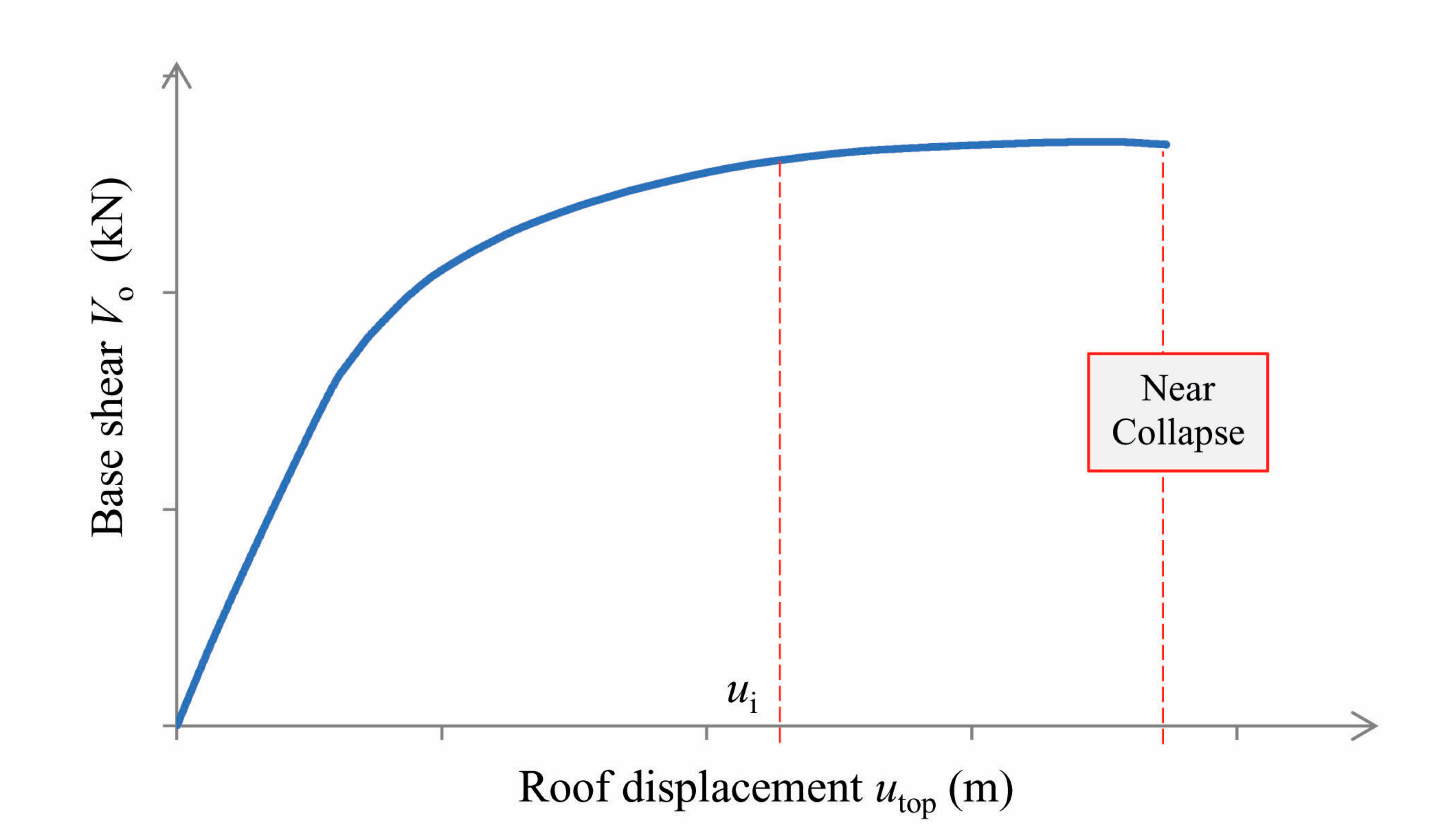
(b): A suitable numerical non-linear model of the structure is obtained, and two pushover analyses are performed, with positive and negative floor forces, leading to the drawing of the capacity curves of the structure in terms of base shear and roof displacement (Figure 1). As regards the floor lateral force pattern used in pushover analysis, the triangular or the first mode pattern of forces is suitable for building structures up to four floors. For higher buildings, an additional second-floor force pattern is proposed with a unit base shear ( $V_{o}$ ), in which an additional force equal to $0.20 \cdot V_{o}$ is applied at the top floor [22] and the rest of the base shear (namely the $0.80 \cdot V_{o}$ ) is distributed (in floor forces) according to the triangular or to the first mode pattern. The goal here is to consider the higher mode effects of tall buildings into the linear and non-linear area, which can be significant especially for more flexible structures, such as moment-frames. Another important point in the application of pushover analysis is that P-D effects should always be considered in the nonlinear area, especially for frame structures which are more flexible.

(c): By performing Modal analysis at each i-step (or at various characteristic steps) of the pushover analysis, using the stiffness matrix of the damaged structure obtained at the last i-step in pushover analysis, the diagram of the instantaneous (step) cyclic Eigen-Frequencies $f_{N, i}$ (in Hz) of the damaged structure is drawn as a function of the roof displacement $u_{t o p, i}$ of the structure (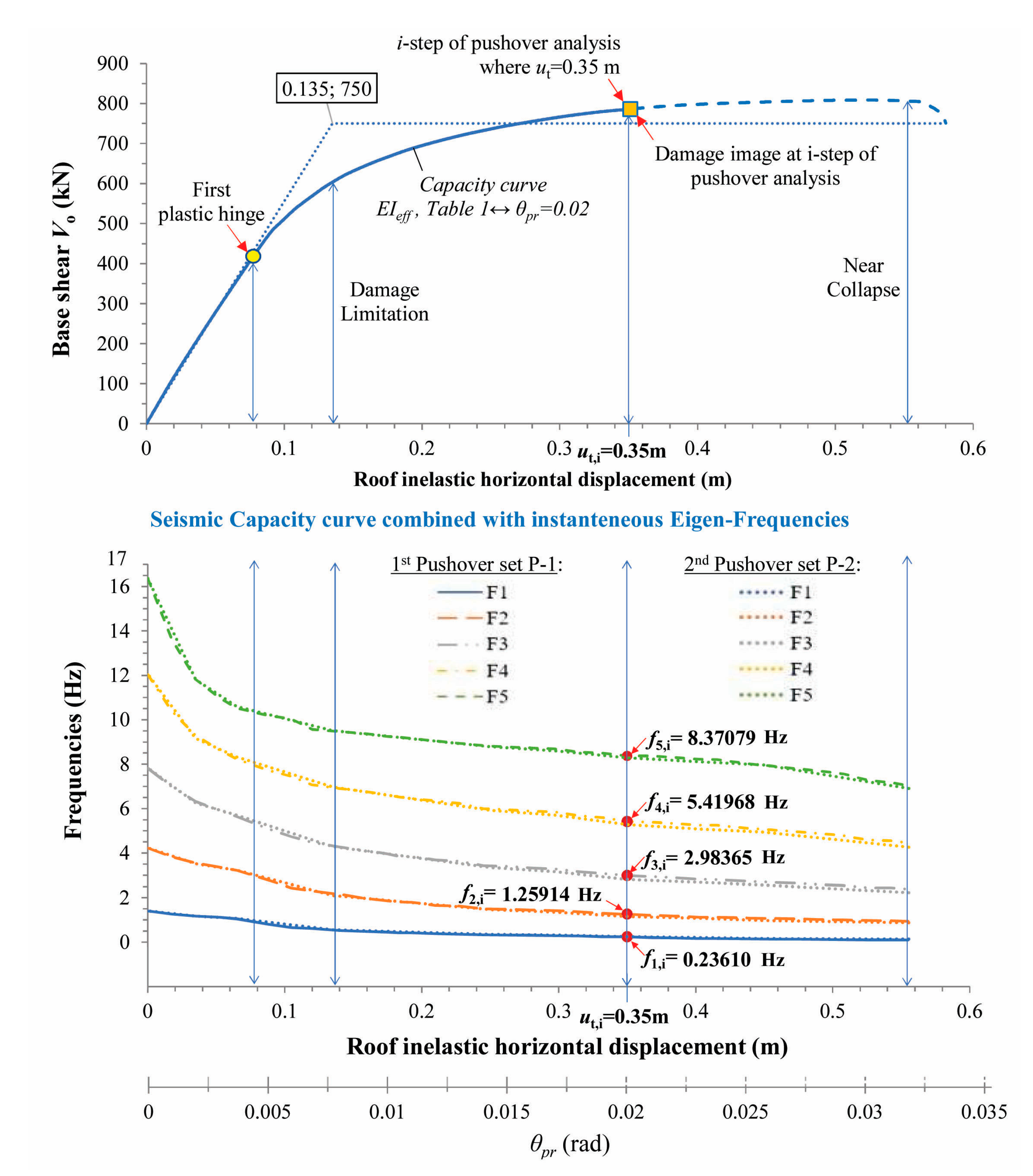Figure 2). In this diagram, that is the novel key point of the proposed methodology, the value of the inelastic roof displacement $u_{t o p, i}$ is the abscissa and the value of the Eigen-Frequencies $f_{N, i}$ of the damaged structure is the ordinate.

It is emphasized that that the sequence of pushover and instantaneous modal analyses of the structure, targeting each time at a gradual increasing roof displacement, should be performed in a nonlinear model of the structure with discrete values

{E_{c} I}_{e f f, i}

(

E_{c}

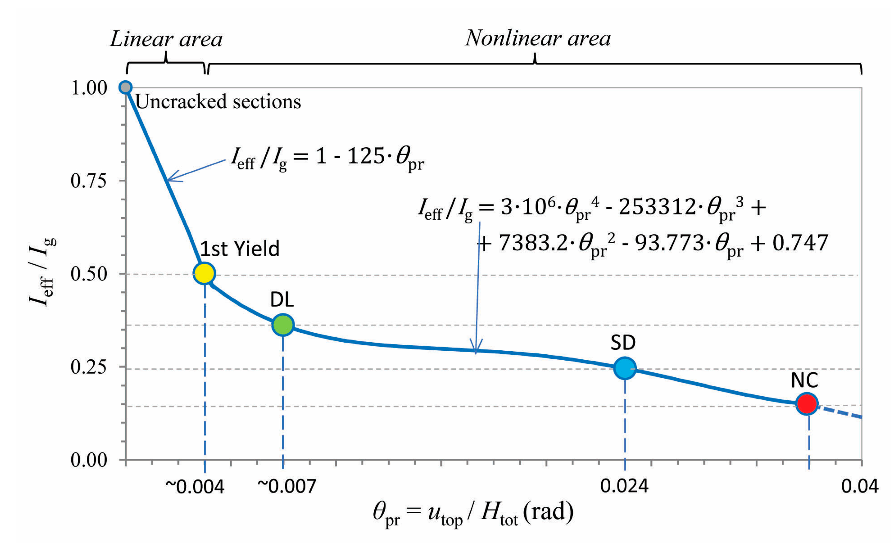
is the elastic modulus of concrete) of the effective bending stiffness of RC structural elements, that correspond to different damage states at each i-step, due to stiffness degradation because of damage. The damage state corresponds to various performance levels: undamaged state, first Yield (first plastic hinge formation), Damage Limitation (DL), Significant Damage (SD), Near Collapse (NC), and all the intermediate ones. Hence, an effective stiffness scenario in terms of the effective moment of inertia ratio

I_{e f f, i} / I_{g}

(where

I_{g}

is the moment of inertia of the geometric section) must be prepared before performing pushover and modal analyses, as a function of the mean (chord) rotation of the frame structure,

θ_{p r, i}

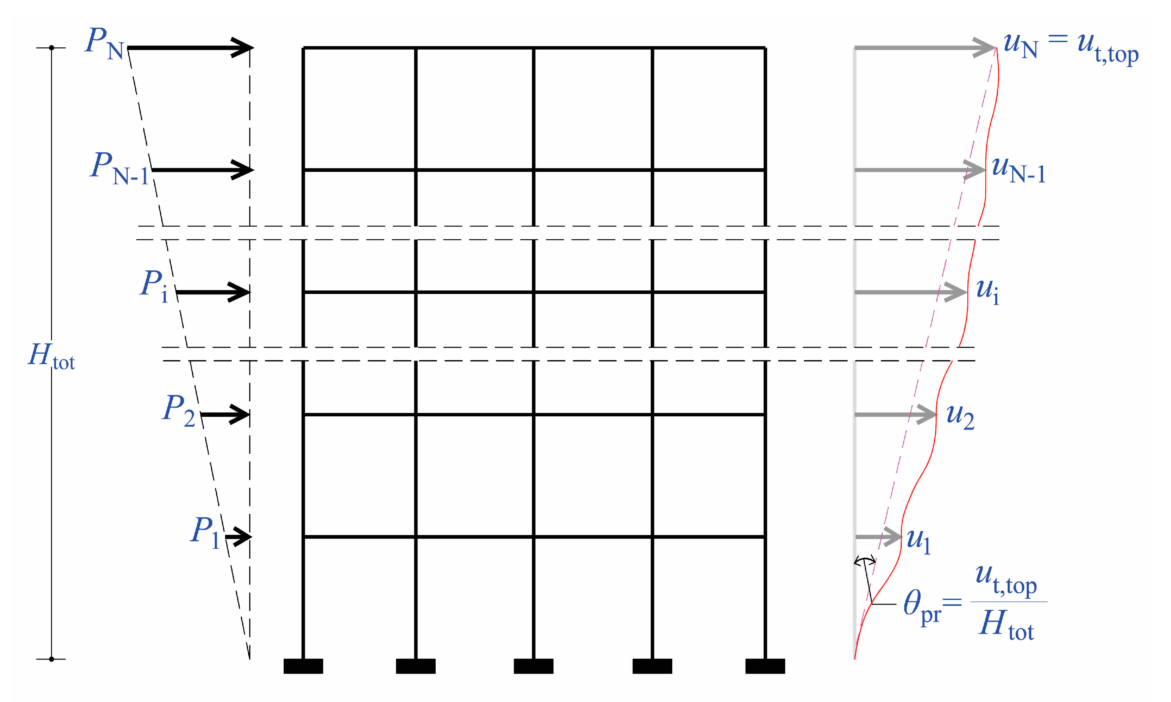
, where the subscript pr,i refers to the chord rotation profile of the moment-frame at the examined i-step. This is equal to

θ_{p r, i} = u_{t, t o p, i} / H_{t o t}

, where

u_{t, t o p, i}

is the seismic (target) roof displacement at the i-step and

H_{t o t}

is the total building height (Figure 3). As shown in Figure 4, the effective moment of inertia

I_{e f f, i}

of RC structural elements (as the mean value for their two end-sections) that corresponds to the NC performance level is too low, and it can be calculated from an equation given in EN 1998-3 [23]:

{E_{c} I}_{e f f} = \frac{M_{p} \cdot L_{v}}{3 \cdot θ_{y}} (8)

where

M_{p}

is the plastic moment of the section determined through an elastoplastic idealization of the Moment-Curvature diagram Μ-φ of the section,

L_{v}

is the shear length of the RC element taken equal to the half clear-length of the element [22,23], and

θ_{y}

is the available chord rotation of the shear length of the element at yield state that is given approximately by Equation A.10 of Eurocode EN 1998-3. In fact, EN 1998-3 impose these low values of the effective bending stiffness on all RC structural elements, in order to perform nonlinear analysis targeting all performance levels, from DL to NC. Since this is too conservative, a scaling is proposed in Figure 4 when pushover analysis targets other higher seismic performance levels, such as DL or SD or all other intermediate ones [22]. Another point in Equation (8) is that it provides different values of effective stiffness at various structural elements. To simplify this, the mean effective stiffness at NC state is assigned to each structural element of the nonlinear model according to the proposed methodology. Moreover, the effective stiffness scenario of Figure 4 proposes discrete

I_{e f f, i} / I_{g}

values from the uncracked state towards the 1^st Yield (when the 1^st plastic hinge is shown) and from there to DL. Additionally, two proposed lines (with the corresponding equations) for the effective stiffness into the linear and nonlinear area are also presented into Figure 4:

For the linear area,

0 \leq θ_{p r} \leq 0.004

I_{e f f} / I_{g} = 1 - 125 \cdot θ_{p r}

(9)

For the nonlinear area,

0.004 < θ_{p r} \leq 0.032

I_{e f f} / I_{g} = 3 \cdot 10^{6} \cdot {θ_{p r}}^{4} - 253312 \cdot {θ_{p r}}^{3} + 7383.2 \cdot {θ_{p r}}^{2} - 93.773 \cdot θ_{p r} + 0.747

(10)

For the nonlinear area in the vicinity of (near) collapse,

0.032 < θ_{p r} :

I_{e f f} / I_{g} = M_{p} \cdot L_{v} / (3 \cdot θ_{y} \cdot E_{c} \cdot I_{g})

(11)

(d): The known fundamental Eigen-Frequency of the damaged structure of phase (a), $f_{1}$ , is inserted in the instantaneous Eigen-Frequencies diagram (Figure 2) and, hence, the respective inelastic seismic (target) roof displacement $u_{i}$ is determined. All the rest instantaneous higher Eigen-Frequencies $({f_{2,}}_{i}, {f_{3,}}_{i}, \dots {f_{N,}}_{i})$ lie on the same vertical line passing through the target-displacement $u_{i}$ .

(e): The damage state of the structure can be identified by the results of two pushover analyses (with floor forces along the positive and negative direction) at the i-step where the roof displacement $u_{i}$ is shown. The location and the state of the plastic hinges at this i-step of each pushover analysis indicate the damaged state of the structure, while the final requested damaged state of the structure will result from the superposition of the damage states of the two pushovers.

(f): Moreover, a linear modal analysis is performed at the i-step of pushover analysis (phase e), using as initial conditions the instantaneous stiffness matrix of the i-step. From this modal analysis, all the circular Eigen-Frequencies $ω_{i, g}$ and all the instantaneous mode-shapes $φ_{i, g}$ of the damaged structure are calculated.

(g): At the end, the instantaneous stiffness matrix $k_{i}$ of the structure at the examined inelastic i-step is determined. Hence, the Damage Stiffness Matrix ${Δ k}_{i}$ at the same i-step is calculated from the general relationship ${Δ k}_{i} = k_{o} - k_{i}$ , where $k_{o}$ is the known Initial Stiffness Matrix of the undamaged structure.

3. Numerical Example

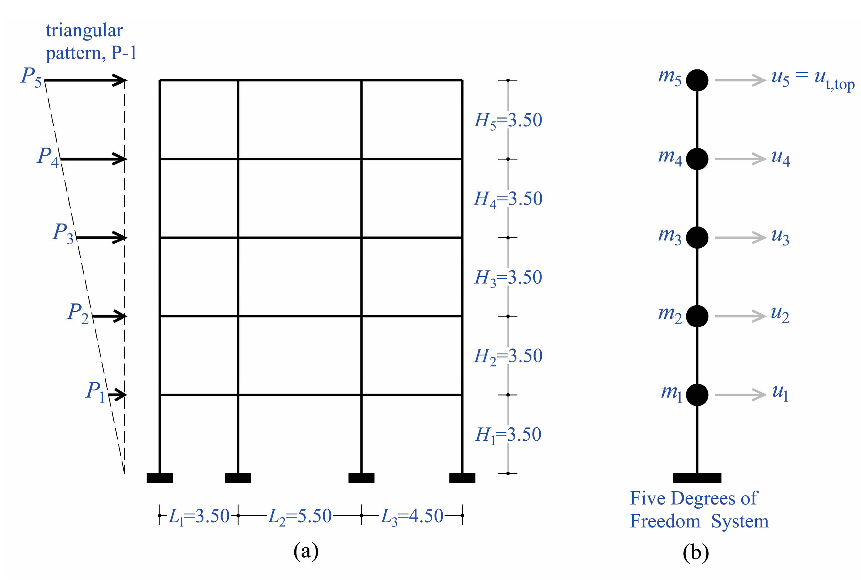
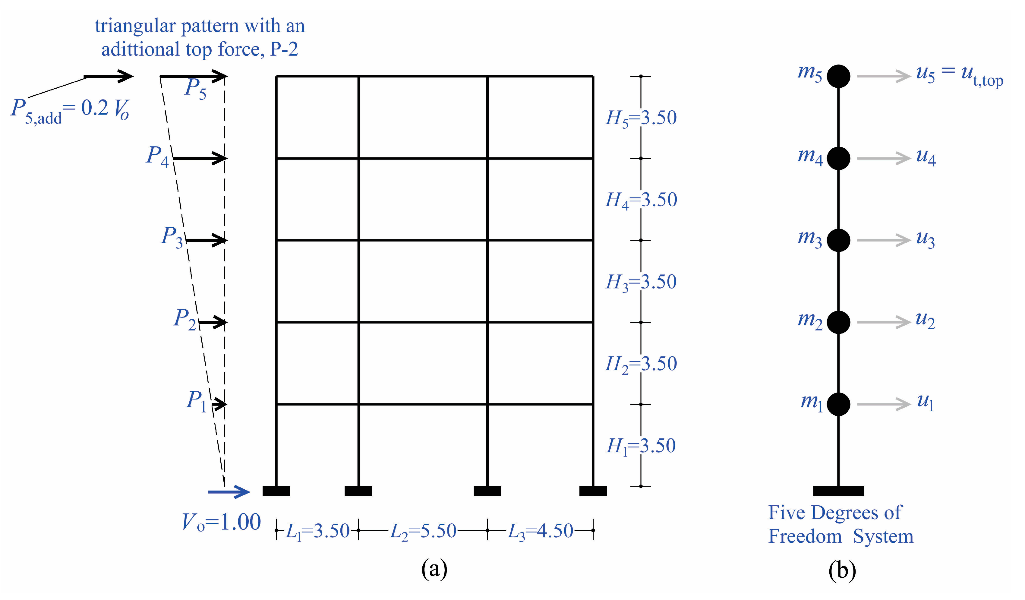
We consider the existing five-storey planar RC frame of Figure 5, with three unequal spans, with dimensions

L_{1} = 3.5 m,

L_{2} = 5.5 m

and

L_{3} = 4.5 m

. The strorey height is equal to 3.5 m in all floors, and the total height of the frame is 17.5 m. The total vertical uniformly distributed loads of the seismic combination

p = g + ψ_{Ε} q

(where

g

is the dead load,

ψ_{Ε} q

is the quasi-live load and

ψ_{Ε} = 0.3

[24]) applied on the spans of each floor are respectively equal to

p_{1} = 28,

p_{2} = 35

and

p_{3} = 32

kN/m. These loads contribute to a floor mass of approximately 45 tn and to a total frame mass of 225 tns. The floor mass and the degrees of freedom of the five-storey planar frame for the modal analysis are illustrated in Figure 5b and Figure 6b. Additionally, Figure 5a and Figure 6a present the two patterns (P-1 and P-2) of lateral floor forces that will be used in pushover analysis. The frame was constructed with concrete grade C25/30 and steel grade B500s, with mean compressive and tensile strengths, respectively equal to

f_{c m} = 33 M P a

and

f_{y m} = 550 M P a

. The Elasticity Modulus of the concrete is equal to

E_{c} = 31 G P a

, while that of the steel is

E_{s} = 200 G P a

. There are two different column sections, with dimensions

b_{c} \times h_{c}

equal to

0.45 \times 0.45

and

0.50 \times 0.50

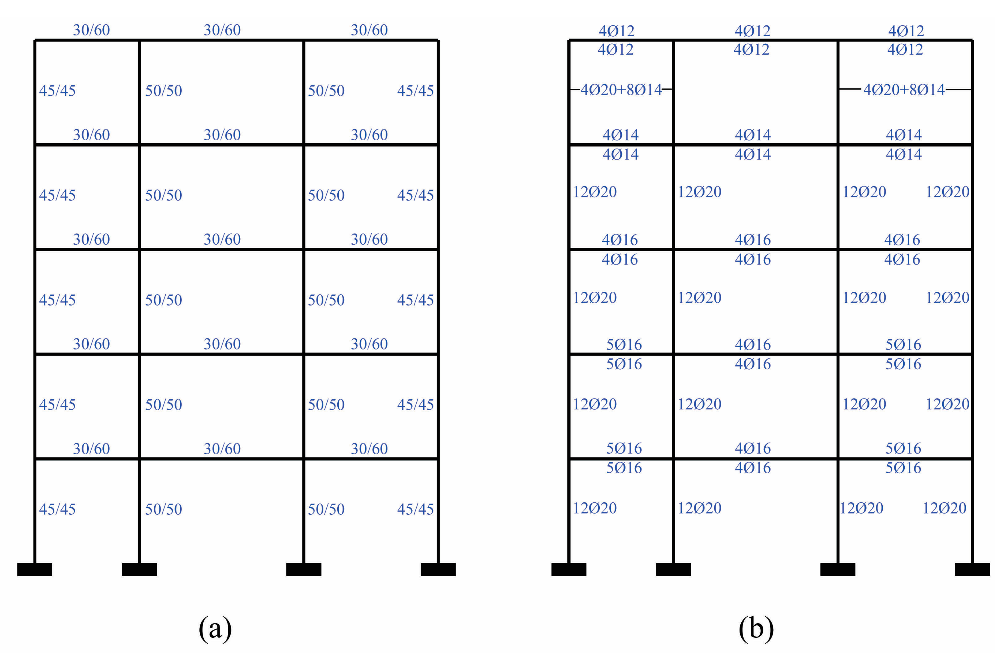
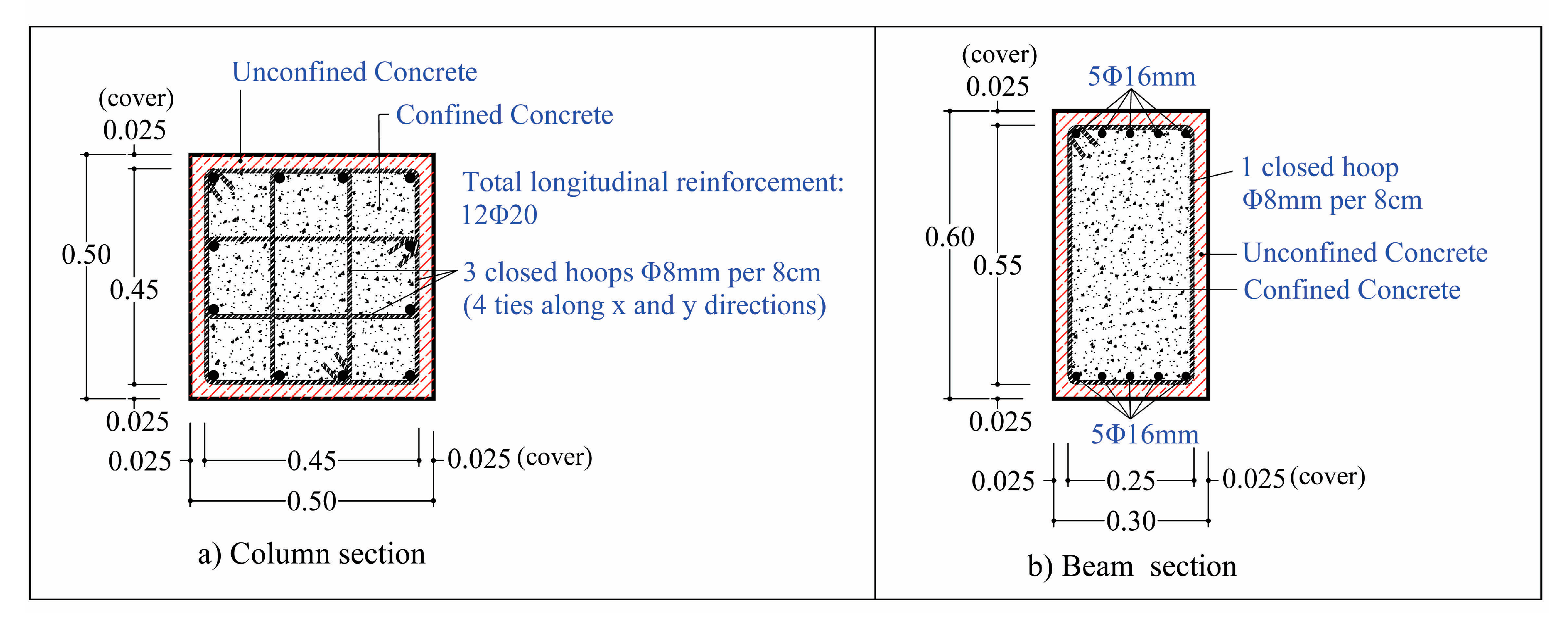
m, respectively. All column sections are symmetrically reinforced with 12 steel bars of 20 mm diameter (or 12Ø20) at all floors, except the top floor where the total steel bars are 4Ø20+8Ø14 (Figure 7). The confinement reinforcement in all columns, in every floor, consists of closed hoops with 4 ties of 8 mm diameter, evenly spaced per 8 cm axially at the critical end sections. The beams of the frame have a rectangular section of dimension

b_{b} \times h_{b} = 0.30 \times 0.60

m and are symmetrically reinforced at the upper and the lower fibers but have different steel bars at various floors (Figure 7). The beams in all floors have a perimetric closed hoop of 8mm diameter, evenly spaced per 8cm axially at the critical end sections, which acts as shear reinforcement and provides a low confinement state. Steel reinforcement details of typical column and beam sections are shown in Figure 8. It is noting that the planar RC frame has been designed according to EN 1998-1 [24] for the high ductility class (DCH) and, hence, it is expected to demonstrate a beam-sway plastic mechanism in the nonlinear area.

In order to apply the proposed methodology [21] for the identification of the structural damage, a sequence of pushover and instantaneous modal analyses should be performed. 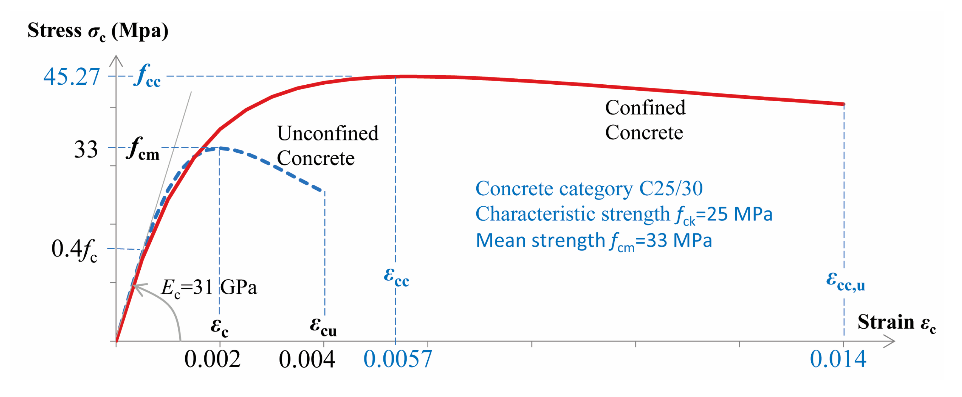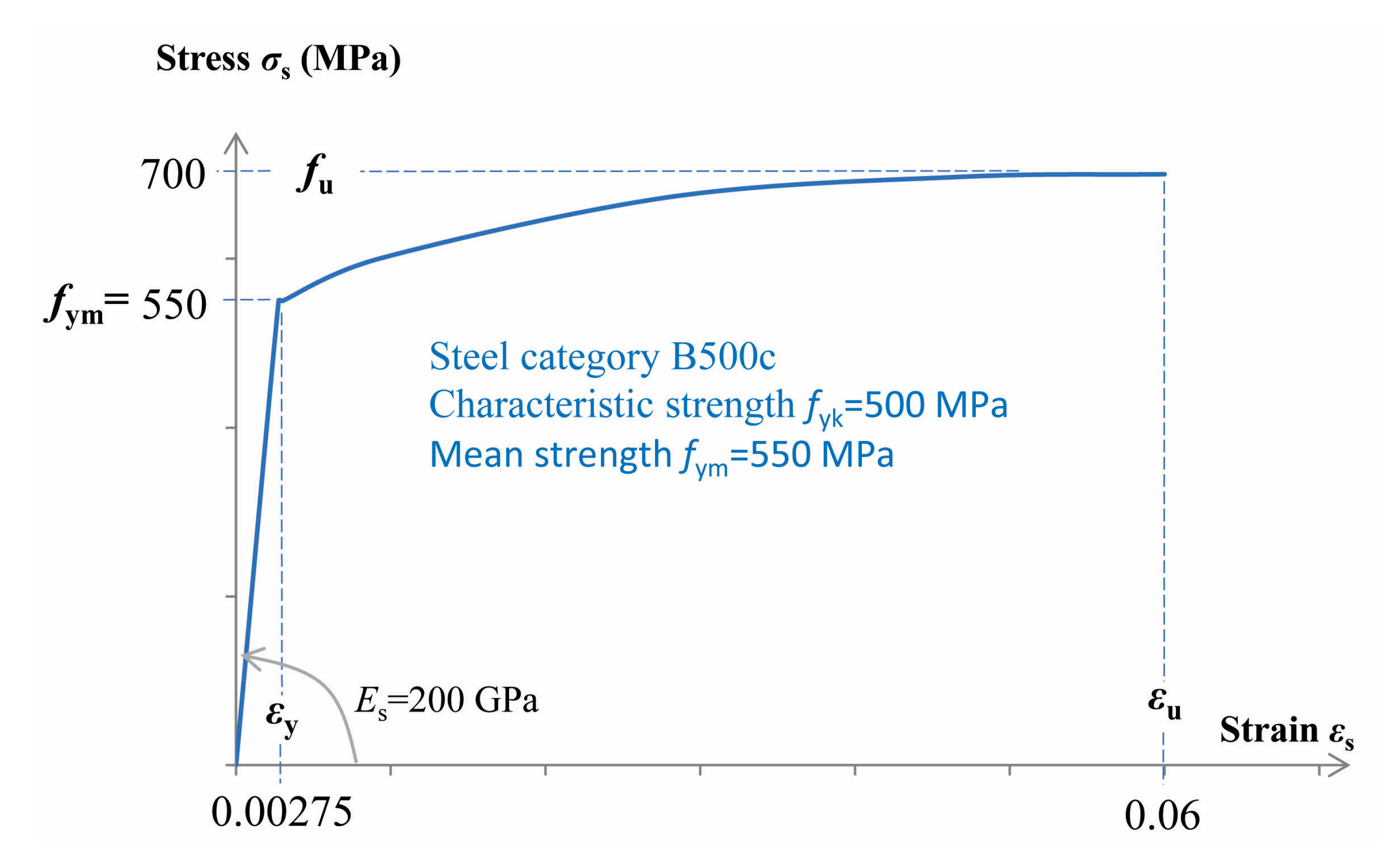The nonlinear model of the planar RC frame was created in the FEM analysis software SAP2000 [25] using fiber hinges to simulate the locations of the possible developing plastic hinges at the end-sections of the elements, with plastic hinge length calculated by Equation (A.9) of EN 1998-3 [23]. The material constitutive relationships used in nonlinear analyses are consistent with: (a) the uniaxial unconfined and confined model for the concrete proposed by Mander, Priestley and Park (1988) [26] (Figure 9), and (b) the steel reinforcement model (parabolic at strain hardening region) proposed by Park and Paulay (1975) [27] (Figure 10).

A section analysis [25] should be performed first, in order to calculate the effective bending stiffness

{E_{c} I}_{e f f f}

of the structural elements at the NC state, using Equation (8). Then, the stiffness scenario used in the sequence of pushover analyses of the frame -with gradually increasing target roof displacement- is established (phase c), which is presented in Table 1 as a function of the profile angle

θ_{p r}

(Figure 3). The discrete values of the effective moment of inertia

I_{e f f}

assigned to all RC structural elements of the nonlinear model of the frame depend on the seismic (target) roof displacement of the pushover analysis, i.e. on the target performance level (Figure 4). For example, if the target roof displacement

u_{t, t o p}

corresponds to a value of

θ_{p r}

equal to 0.028, i.e.

u_{t, t o p} = θ_{p r} \cdot H_{t o t} = 0.028 \cdot 17.5 = 0.49 m

, then the value of

I_{e f f}

that should be assigned to all structural elements of the nonlinear model is equal to

0.19 I_{g}

according to Table 1.

To obtain the capacity curve of the planar frame, two pushover analyses are performed targeting the NC state, with positive and negative signs of the floor lateral forces. In these analyses, the effective moment of inertia

I_{e f f}

of Table 1 that correspond to the NC state is used (Equation 8), i.e. the value 0.15

I_{g}

. Since the planar frame has more than four floors, two floor force patterns are used in pushover analysis according to phase (b): (i) the triangular pattern (Figure 5a), (ii) the triangular pattern but with an additional top force equal to

0.20 \cdot V_{o}

for a unit base shear (

V_{o} = 1.00 k N,

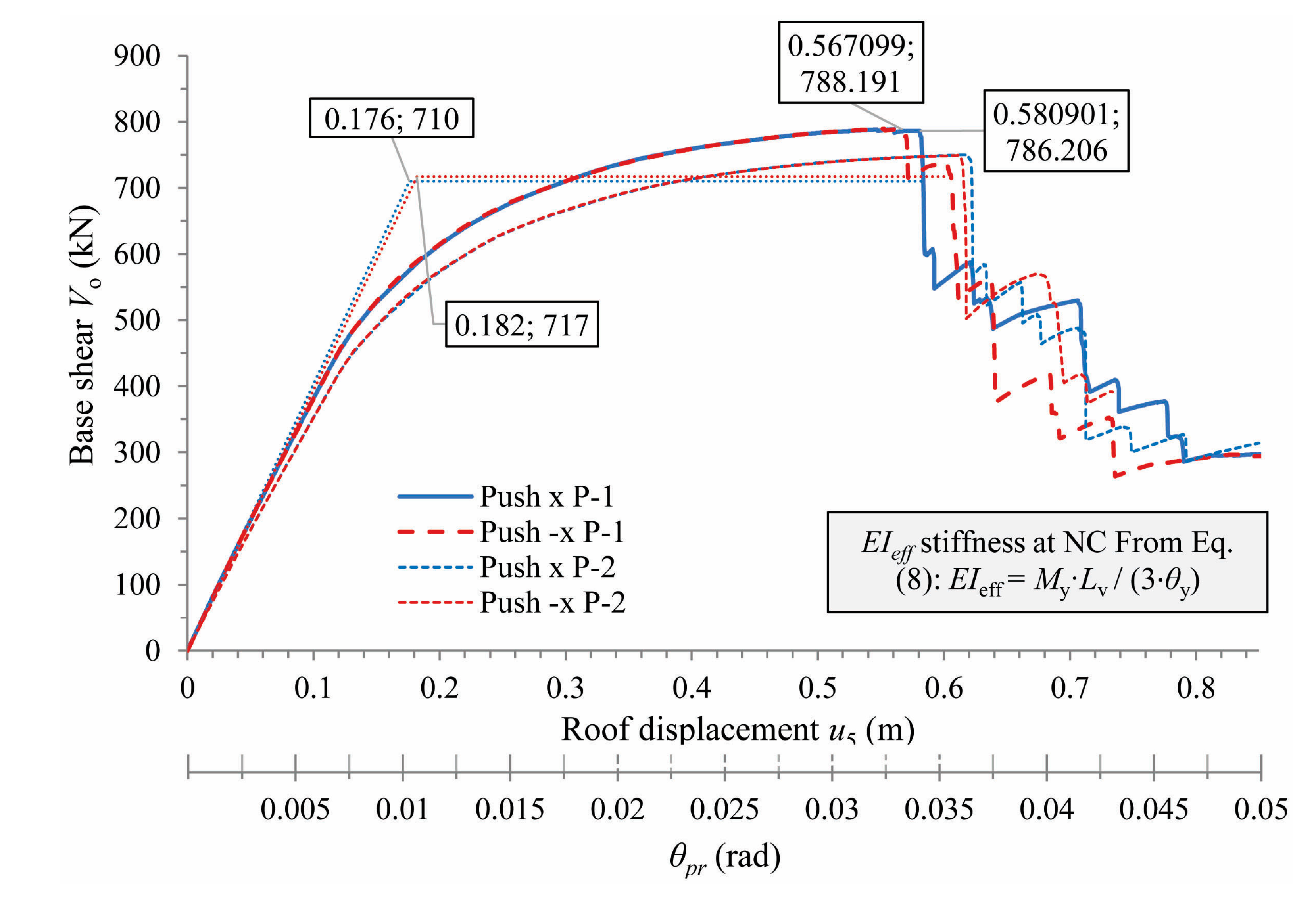
Figure 6a). These two force patterns will be referred to, from now on, as P-1 and P-2. The two capacity curves of the planar frame for the two pushover sets are illustrated in Figure 11, together with bi-linearization lines for the first set P-1 that mark the DL state at a value of

θ_{p r}

about equal to

0.01 r a d

. As shown in this figure, the NC state of the frame is conservatively shown at a value of

θ_{p r}

equal to

0.56 / 17.5 = 0.032 r a d

, i.e., that in the last line of Table 1. The capacity curves for the second pushover set P-2 present higher ultimate displacements and lower elastic stiffness.

Next, a sequence of pushover analyses of the existing planar frame is performed, where each one targets a seismic roof displacement which corresponds to the discrete values of the profile angle

θ_{p r}

of Table 1, from 0 to 0.032 rad. In each pushover analysis, the effective moment of inertia

I_{e f f}

assigned to the structural elements of the nonlinear model of the frame is that shown in Table 1, which corresponds to the same discrete values of the target profile angle

θ_{p r}

. At the last step of the separate pushover analyses, an instantaneous modal analysis is running with initial condition the damage state of this last step, i.e. using the stiffness matrix of the damaged frame at the last step of each pushover analysis. From the sequence of modal analyses of the planar frame, the instantaneous cyclic Eigen-Frequencies of the system are recorded (F₁ to F₅) and the diagram of the instantaneous cyclic Eigen-Frequencies (in Hz) of the planar frame in the nonlinear area is obtained as a function of the roof displacement

u_{5}

. This is done for the two directions of application of the floor forces and the mean values of the instantaneous cyclic Eigen-Frequencies (in Hz) of the planar frame are calculated, for both pushover sets with the different floor force patterns P-1 and P-2. In Figure 12, the diagram of the instantaneous cyclic Eigen-Frequencies (in Hz) is combined with the capacity curve of the planar RC frame. For figure clarity, only one capacity curve is presented, that for the pushover with positive floor forces following a triangular pattern (P-1). This curve was determined using a nonlinear model of the frame in which the

I_{e f f}

value of Table 1 that corresponds to

θ_{p r} = 0.02 r a d

has been assigned to all RC structural elements. As is shown in Figure 12, the two pushover sets P-1 and P-2 provide similar results for the instantaneous cyclic Eigen-Frequencies in this planar frame. At

θ_{p r} = 0.02 r a d

, the second pushover set (P-2) provides a value for f₁ (Hz) which is 3% higher while for the other frequencies lower values up to 8% are shown. Generally speaking, the difference for f₁ (Hz) increase linearly with the damage state for the second pushover set, up to 30% at the NC state. Finally, the mean values of the instantaneous cyclic Eigen-Frequencies (Hz) of the multi-storey frame resulted from four pushovers along the positive and negative directions (P-2 and P-3) should be used in the diagram.

According to phase (a) of the methodology for existing structures, an identification multi-channel system of uniaxial accelerometers is installed in the 5-storey planar RC frame and response accelerations when the frame is quasi-calm are recorded. From the analysis of the records, the fundamental Eigen-Frequency

f_{1, i} = 0.23610 H z

for the i-step of pushover analysis is determined.

Then, according to phase (d) of the methodology, the fundamental Eigen-Frequency

f_{1, i}

is inserted in the Eigen-Frequencies diagram of Figure 12 (see also the key-Figure 2) and the respective displacement

u_{5, i} = 0.35 m

of the frame roof is determined, which corresponds to

θ_{p r} = 0.02 r a d

. All the other higher frequencies (

f_{2, i} t o f_{5, i}

) can also be found from Figure 12 at the same i-step. The first three instantaneous mode shapes (φ_1,i to φ_3,i) of the multi-storey frame at the corresponding i-step where

θ_{p r}

is equal to 0.02 rad are illustrated in Figure 13. Moreover, at the i-step of the pushover analyses where the roof displacement

u_{5, i}

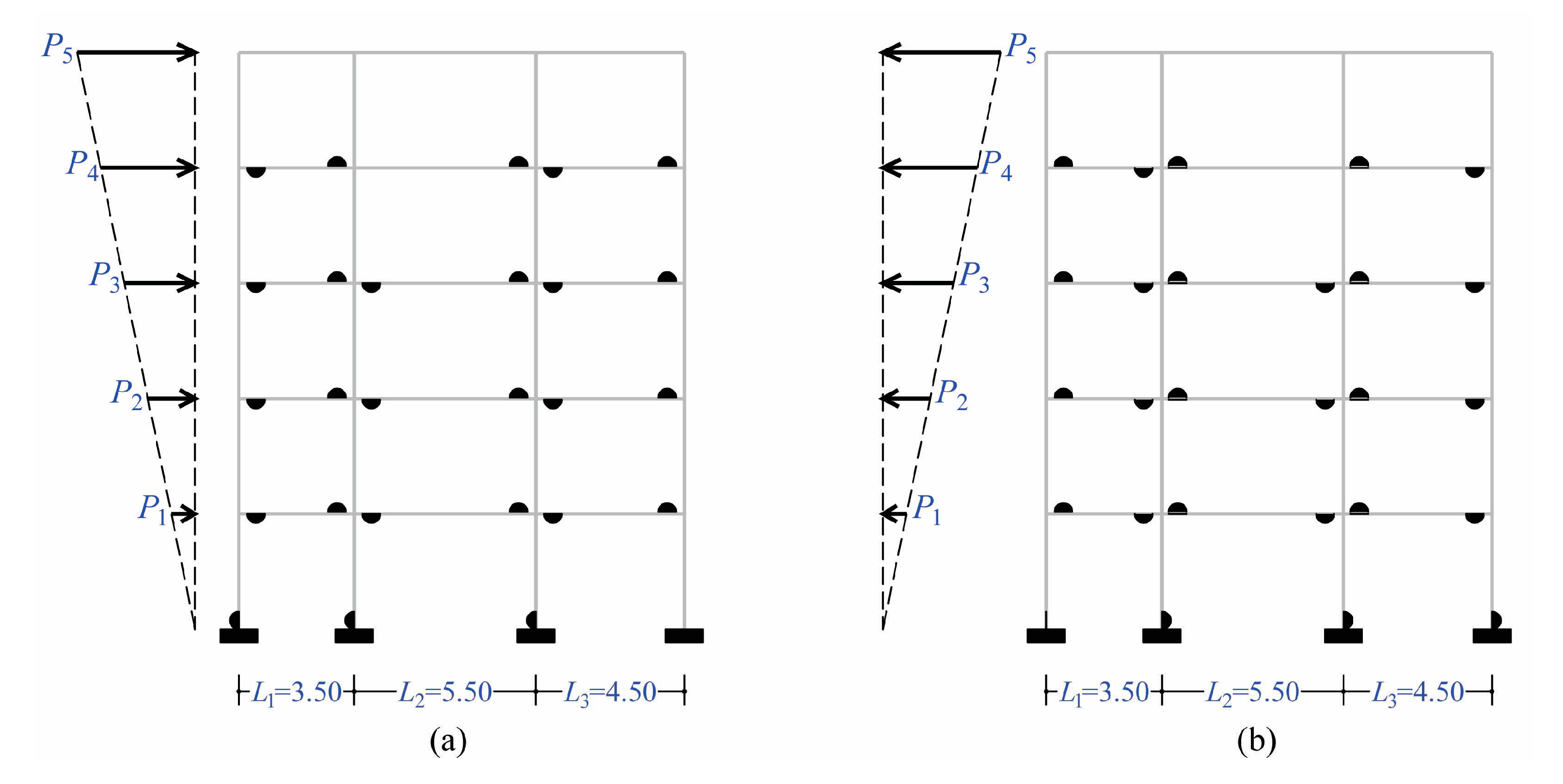
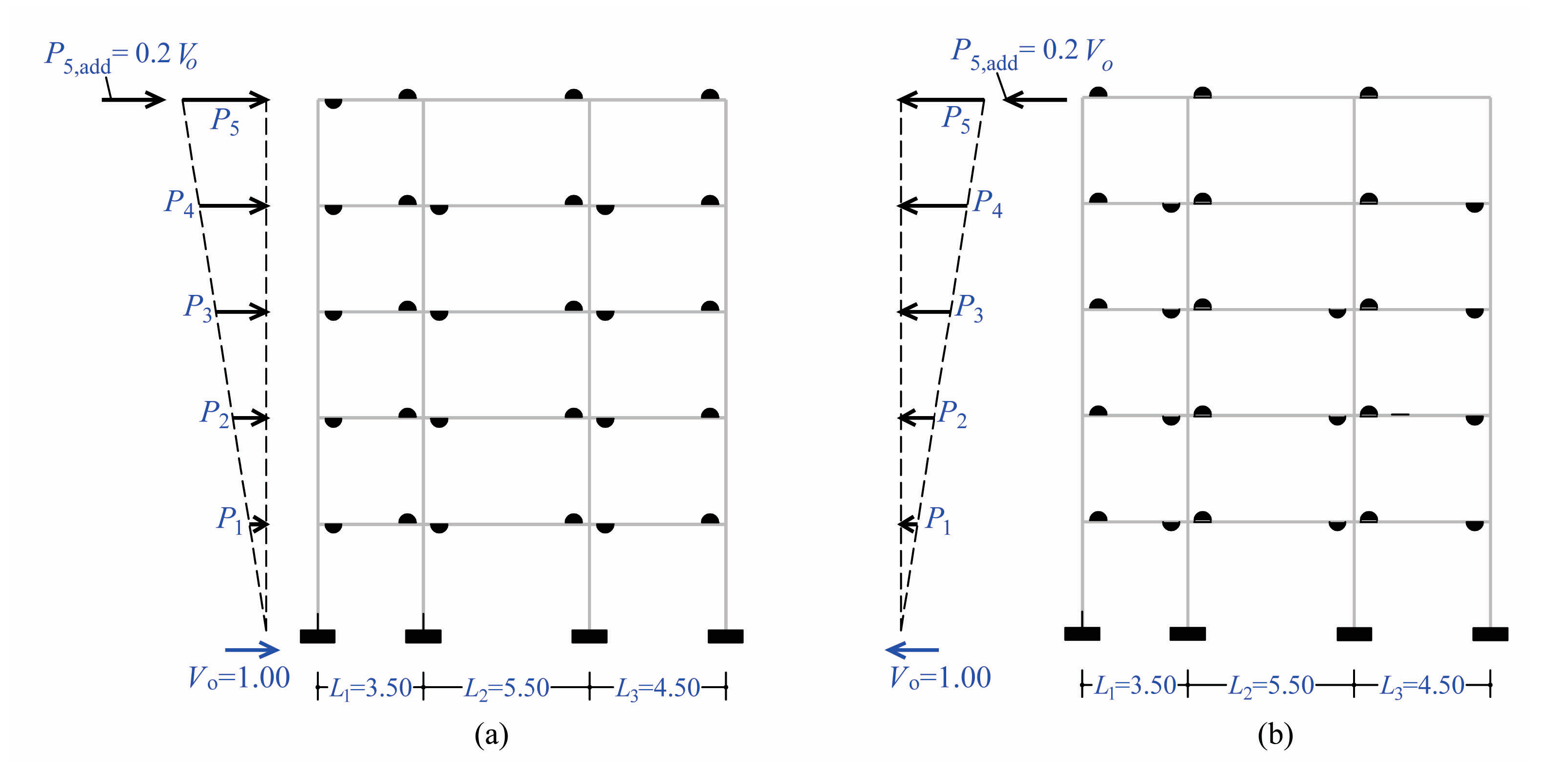
appears, two damage images are obtained, one for the positive and one for the negative application of floor forces, for each one of the two pushovers sets P-1 and P-2. By these two damage images for each one pushover set and by taking the envelope damage image from the two sets, the final requested estimation of the damage is obtained. In Figure 14 the damage image for the first pushover set P-1 is shown, separately for the positive and negative direction of the lateral floor forces. In this figure, the developed plastic hinges are illustrated with a black semicircle at the upper or lower fibers of the beams. As shown in this figure, the multi-storey planar frame develops a beam-sway type plastic mechanism, with plastic hinges at the end-sections of the beams in all floors (except the top floor) and at the base of the columns of the ground floor. Τhis is fully in line with the seismic design objective for high ductility [24]. For the second set P-2 of pushover analysis, the damage is distributed throughout the frame, at the end-sections of the beams in all floors, but the magnitude of damage is a little higher in the upper half of the frame and a little lower in the lower half (Figure 15). Also, no plastic hinges appear at the base of the columns of the ground floor.

It is noting that in an earthquake event, the actual seismic load on the structure is different and this loading varies in each time step. Hence, the damage distribution on the frame can be different from that obtained by the pushover analysis. However, the critical parameter in the recently proposed methodology is the fundamental Eigen-Frequency, which is identified by monitoring with a local network of uniaxial accelerometers. Knowing the fundamental Eigen-Frequency of the structure, the equivalent lateral displacement of the monitoring point on the roof of the building can be estimated by Figure 12 and then the capacity curve is considered to identify the damage state. On the other hand, the second set of pushover analysis, with the load pattern with an additional top force, should always be considered in tall moment-frames with more than four floors, to take account of the higher mode effects on the damage potential. In this frame, both pushover sets provide similar values for the fundamental instantaneous cyclic Eigen-Frequency

f_{1, i}

and for the damage image, but, if the frame was taller, then these results might have been different.

Finally, according to phase (g) of the methodology, the instantaneous stiffness matrix

k_{i}

of the frame structure at the examined inelastic i-step (

θ_{p r} = 0.02 r a d

) is calculated for the case of pushover analysis with positive floor forces following the triangular pattern (P-1):

k_{i} = [\begin{matrix} 36370.51 & - 33082.10 & 14643.09 & - 3673.87 & 679.84 \\ - 33082.10 & 50479.70 & - 38748.17 & 15118.43 & - 2690.79 \\ 14643.09 & - 38748.17 & 52466.20 & - 36198.25 & 10206.16 \\ - 3673.87 & 15118.43 & - 36198.25 & 43966.32 & - 19808.32 \\ 679.84 & - 2690.79 & 10206.16 & - 19808.32 & 11722.76 \end{matrix}]

Therefore, the Damage Stiffness Matrix

{Δ k}_{i}

at the same i-step is calculated from the general relationship

{Δ k}_{i} = k_{o} - k_{i}

, where

k_{o}

is the known Initial Stiffness Matrix of the planar frame in the health state without damage. The later can be calculated from the nonlinear model of the frame in which the geometric moment of inertia

I_{g}

has been assigned to all RC structural elements and the gravity loads are applying gradually:

k_{o} = [\begin{matrix} 257837.85 & - 150932.01 & 37561.89 & - 5540.92 & 712.70 \\ - 150932.01 & 225406.70 & - 140857.01 & 33129.35 & - 3282.19 \\ 37561.89 & - 140857.01 & 207019.25 & - 118543.59 & 20706.76 \\ - 5540.92 & 33129.35 & - 118543.59 & 152434.25 & - 62373.91 \\ 712.70 & - 3282.19 & 20706.76 & - 62373.91 & 44252.75 \end{matrix}]

Hence, the Damage Stiffness Matrix

{Δ k}_{i}

of the planar frame, at the same i-step, is calculated as following:

{Δ k}_{i} = k_{o} - k_{i} = [\begin{matrix} 221467.34 & - 117849.92 & 22918.80 & - 1867.05 & 32.86 \\ - 117849.92 & 174926.99 & - 102108.84 & 18010.92 & - 591.40 \\ 22918.80 & - 102108.84 & 154553.05 & - 82345.34 & 10500.60 \\ - 1867.05 & 18010.92 & - 82345.34 & 108467.94 & - 42565.59 \\ 32.86 & - 591.40 & 10500.60 & - 42565.59 & 32529.99 \end{matrix}]

For the pushover analysis with positive floor forces following the triangular pattern but with an additional top force (P-2), the corresponding Damage Stiffness Matrix

{Δ k}_{i}

of the planar frame, at the same i-step (

θ_{p r} = 0.02 r a d

), is calculated as abovementioned and is equal to:

{Δ k}_{i} = [\begin{matrix} 219118.62 & - 117522.85 & 22932.98 & - 1948.18 & 110.79 \\ - 117522.85 & 175015.31 & - 102488.80 & 18377.29 & - 872.53 \\ 22932.98 & - 102488.80 & 155574.83 & - 84085.17 & 11567.50 \\ - 1948.18 & 18377.29 & - 84085.17 & 114674.18 & - 47323.23 \\ 110.79 & - 872.53 & 11567.50 & - 47323.23 & 36434.37 \end{matrix}]

4. Discussion

Knowing the Damage Stiffness Matrix

{Δ k}_{i}

of the planar frame, the final percentage deviation terms of

{Δ k}_{i}

can be calculated with respect to the Initial Stiffness Matrix

k_{o}

and are presented in matrix form in Table 2 and Table 3 respectively for the P-1 and P-2 force patterns. The visual representation of these tables is shown in Figure 16 and Figure 17, respectively. These deviations on the diagonal terms of the Damage Stiffness matrix indicate the degree of damage of the planar five-storey RC frame at the i-step where

θ_{p r} = 0.02 r a d

(

u_{5} = 0.35 m

), which is fully compatible with the damage images of Figure 14 and Figure 15. We also notice that in Table 3 (P-2 pattern) the values of the terms in the damage stiffness matrix

{Δ k}_{i}

that correspond to the upper half of the frame (degrees of freedom

u_{4}

u_{5}

) are higher while those corresponding to the lower half of the frame (degrees of freedom

u_{1}

u_{2}

) are lower relative to the respective ones in Table 2 (P-1 pattern). The values of

{Δ k}_{i}

that correspond to

u_{3}

(intermediate floor) are about the same in both tables. Hence, the form as well as the values of the damage stiffness matrix

{Δ k}_{i}

is fully compatible with the damage image of Figure 14 and Figure 15. The final Damage Stiffness Matrix

{Δ k}_{i}

, which mark the damage state of this planar RC frame, will be determined as the average of the corresponding values resulted from the two patterns P-1 and P-2 (Figure 16 and Figure 17).

u_{1}

u_{2}

u_{3}

u_{4}

u_{5}

u_{1}

u_{2}

u_{3}

u_{4}

u_{5}

u_{1}

u_{2}

u_{3}

u_{4}

u_{5}

u_{1}

u_{2}

u_{3}

u_{4}

u_{5}

5. Conclusions

A recently proposed methodology [21] for the identification of damage in RC frame structures is validated in the present paper by examining a group of planar, ductile, multi-storey RC moment-frames, from which a numerical example has been presented here. This is a five-storey planar moment-frame with three unequal spans which develops a beam-sway plastic mechanism. The proposed methodology uses a hybrid technique, that is called “M and P technique” (where the M means “Monitoring” and the P means “Pushover”), where the pushover capacity curve of the multi-storey frame is combined with the diagram of the Instantaneous Eigen-Frequencies of the structure as a function of the inelastic seismic (target) roof displacement. Τhis diagram has been resulted by performing a sequence of pushover and instantaneous modal analyses, with gradually increasing target displacement, and with appropriate values of the effective bending stiffness

E_{c} I_{e f f, i}

of RC structural elements as a function of the target displacement. This gradually increasing target displacement corresponds at each i-step to a specific value of the mean (chord) rotation

θ_{p r, i}

of the moment-frame. By inserting in this diagram, the fundamental Eigen-Frequency of the damaged frame determined by a monitoring network of accelerograms, the roof target displacement of the frame arises and, hence, the damage image of the frame at the corresponding i-step of pushover analysis. Moreover, the instantaneous stiffness matrix and the damage stiffness matrix of the frame at the same i-step of pushover analysis is calculated. The latter is fully compatible with the degree of damage in the multi-storey frame at this i-step of pushover analysis. In this article, pushover analysis has been performed using two patterns of lateral floor forces (the second one with an additional top force) to account for the equivalent results due to the higher mode effects in tall moment frames. Finally, all results cοme as the average of four pushovers along the positive and negative direction.

Therefore, using the proposed methodology for damage identification, a very good estimation of the distribution and of the magnitude of the damage in beam-sway, ductile, multi-storey, planar RC frames has been achieved.

Author Contributions

Conceptualization, T.M., A.B.; methodology, T.M.; software, T.M., A.B.; validation, T.M., A.B.; formal analysis, T.M., A.B.; investigation, T.M., A.B.; resources, T.M., A.B.; data curation, T.M., A.B.; writing—original draft preparation, A.B.; writing—review and editing, T.M., A.B.; visualization, T.M., A.B.; supervision, T.M.; project administration, T.M.; funding acquisition, None. All authors have read and agreed to the published version of the manuscript.

Funding

This research received no external funding.

Data Availability Statement

The data presented in this study are available in the article.

Conflicts of Interest

The authors declare no conflict of interest.

References

Basseville, M.; Benveniste, A.; Goursat, M.; Hermans, L.; Mevel, L.; Auweraer, H. Output-only Subspace-based structural identification: from theory to industrial testing practice. Journal of Dynamic Systems, measurement and Control, Transactions of the ASME 2001, Special issue on identification of mechanical systems 4(123), pp. 668–76. [CrossRef]
Brincker, R.; Zhang, L.; Andersen, P. Modal identification of output-only systems using frequency domain decomposition. Smart Materials and Structures Journal, 2001; 10, 441–445. [Google Scholar] [CrossRef]
Peeters, B. Identification and damage detection in civil engineering. Ph.D. Thesis, Katholieke Universiteit, Leuven, Belgium, 2000. [Google Scholar]
Peeters, B.; Roek, G. Stochastic System Identification for Operational Modal Analysis: A Review. Journal of Dynamic Systems Measurement and Control, 2001. [Google Scholar] [CrossRef]
Wenzel, H.; Pichler, D. Ambient Vibration Monitoring, John Wiley & Sons, Ltd: England, 2005. [CrossRef]
Overschee, P.; De Moor, B. Subspace Identification for Linear Systems: Theory-Implemented-Applications, Kluwer Academic Publishers: Dordrecht, The Netherlands, 1996. [CrossRef]
Papoulis, A. Signal Analysis, International Student Edition, McGraw-Hill Book: USA, 1985.
Oppenheim, A.; Schafer, R. Digital Signal Processing, Prentice-Hall, Inc, Publication: Englewood Cliffs, NJ, New Jersey, 1999. https://research.iaun.ac.ir/pd/naghsh/pdfs/UploadFile_2230.
Bendat, J.; Piersol, A. Random Data. Analysis and Measurement Procedures, Fourth Edition; John Wiley & Sons, Inc Publication: USA, 2010. [Google Scholar]
Makarios, T. Identification of the mode shapes of spatial tall multi-storey buildings due to earthquakes. The new "modal time-histories” method. Journal of the Structural Design of Tall & Special Buildings, 2012; 21, 621–641. [Google Scholar] [CrossRef]
Dragos, K.; Makarios, T.K.; Karetsou, I.; Manolis, G.D.; Smarsly, K. Detection and Correction of Synchronization-induced Errors in Operational Modal Analysis. Journal of Archive of Applied Mechanics, Springer, 2020; 90, 1547–1567. [Google Scholar] [CrossRef]
Zimmerman, D.C.; Kaouk, M. Structural damage detection using a minimum rank update theory. Journal of Vibration and Acoustics, 1994; 116, 222–231. [Google Scholar] [CrossRef]
Kaouk, M.; Zimmerman, D.C. Structural damage assessment using a generalized minimum rank perturbation theory. AIAA Journal, 1994. [Google Scholar] [CrossRef]
Domaneschi, M.; Limongelli, M.P.; Martinelli, L. Damage Identification in a benchmark Cable-Stayed Bridge using the Interpolation Method. In Proceedings of the 7th European Workshop on Structural Health Monitoring, La Cité, Nantes, France, 2014. https://www.researchgate.net/publication/281947001_Damage_Identification_in_a_Benchmark_Cable-Stayed Bridge Using_the_Interpolation_Method, July 8-11.
Domaneschi, M.; Limongelli, M.P.; Martinelli, L. Damage detection and localization on a Cable-Stayed Bridge. Earthquake and Structures, 2015; 5. [Google Scholar] [CrossRef]
Nazari, F.; Baghalian, S. A new Method for Damage Detection in symmetric beams using artificial neural network and Finite Element Method. International Journal of Engineering & Applied Sciences (IJEAS), /: Issue 2, pp. 30-36. https, 2011; 2. [Google Scholar]
Amani, M.G.; Riera, J.D.; Curadelli, R.O. Identification of changes in the stiffness and damping matrices of linear structures through ambient vibrations. Structural Control and Health Monitoring Journal, 2007. [Google Scholar] [CrossRef]
Zhang, S.; Wang, H.; Wang, W.; Chen, S. Damage Detection in Structures Using Artificial Neural Networks. In Proceedings of the International Conference on Artificial Intelligence and Computational Intelligence, Sanya, China, 2010, Oct. 23-24; pp. 207–210. [CrossRef]
Reuland, Y.; Martakis, P.; Chatzi, E. A Comparative Study of Damage-Sensitive Features for Rapid Data-Driven Seismic Structural Health Monitoring. Appl. Sci. 2023. [Google Scholar] [CrossRef]
Martakis, P.; Reuland, Y.; Stavridis, A.; Chatzi, E. Fusing damage-sensitive features and domain adaptation towards robust damage classification in real buildings. Soil Dynamics and Earthquake Engineering 2023, 166. [Google Scholar] [CrossRef]
Makarios, T. Damage Identification in plane multi-storey reinforced concrete frame. The Open Construction & Building Technology Journal, 2023. [Google Scholar] [CrossRef]
Bakalis, A.; Makarios, T. Seismic Enforced-Displacement pushover procedure on multistorey R/C buildings. Engineering Structures 2021, 229. [Google Scholar] [CrossRef]
EN 1998-3. Eurocode 8: Design of Structures for Earthquake Resistance—Part 3: Assessment and Retrofitting of Buildings; European Committee for Standardization: Brussels, Belgium, 2005. [Google Scholar]
EN 1998-1. Eurocode 8: Design of Structures for Earthquake Resistance—Part 1: General Rules, Seismic Actions and Rules for Buildings; European Committee for Standardization: Brussels, Belgium, 2004. [Google Scholar]
Structural Analysis Program SAP2000v23. 2021. Computers and Structures, Inc. www.csiamerica.com.
Mander, J.B.; Priestley, M.J.N.; Park, R. Theoretical Stress-Strain Model for Confined Concrete. Journal of Structural Engineering, /: 114, No. 8, Paper No. 22686, pp. 1804-1826. https, 1988; 8. [Google Scholar]
Park, R.; Paulay, T. Reinforced concrete structures, John Wiley & Sons, Inc.: New York, USA, 1975.

Figure 1. Pushover Capacity Curve of the multi-storey planar frame structure.

Figure 2. Instantaneous Eigen-Frequencies diagram, in the nonlinear area.

Figure 3. The profile angle

θ_{p r}

of the frame structure in pushover analysis with floor lateral forces.

Figure 3. The profile angle

θ_{p r}

of the frame structure in pushover analysis with floor lateral forces.

Figure 4. Effective moment of inertia ratio

I_{e f f} / I_{g}

with reference to the geometric moment of inertia

I_{g}

of RC structural elements at discrete damage states as a function of the mean (chord) rotation of the frame structure

θ_{p r}

(rad).

Figure 4. Effective moment of inertia ratio

I_{e f f} / I_{g}

with reference to the geometric moment of inertia

I_{g}

of RC structural elements at discrete damage states as a function of the mean (chord) rotation of the frame structure

θ_{p r}

(rad).

Figure 5. Five-storey planar RC frame with three unequal spans: (a) static simulation for the first pushover set (P-1) with a triangular force pattern, (b) dynamic simulation.

Figure 6. (a) Static simulation of the five-storey planar RC frame for the second pushover set (P-2) with a triangular force pattern and an additional top force, (b) dynamic simulation.

Figure 7. (a) Sections of RC structural elements, (b) longitudinal steel bars.

Figure 8. Steel reinforcement details of typical column and beam sections.

Figure 9. Stress-strain diagram for unconfined and confined concrete.

Figure 10. Stress-strain diagram for steel bars.

Figure 11. Capacity curves of the planar frame along the +x and -x axis (

{E I}_{e f f}

at NC, Table 1), for the two force patterns P-1 & P-2.

Figure 11. Capacity curves of the planar frame along the +x and -x axis (

{E I}_{e f f}

at NC, Table 1), for the two force patterns P-1 & P-2.

Figure 12. Diagram of the instantaneous Eigen-Frequencies in Nonlinear Area combined with the Seismic Capacity Curve for the two pushover sets.

Figure 13. The first three instantaneous modes φ_1,i to φ_3,i at

θ_{p r} = 0.02

rad.

Figure 13. The first three instantaneous modes φ_1,i to φ_3,i at

θ_{p r} = 0.02

rad.

Figure 14. Plastic mechanism of the planar RC moment-frame by the 1^st set P-1 of pushover analysis, with (a) positive and (b) negative signs of floor forces, at seismic (target) displacement 0.35 m (

θ_{p r} = 0.02 r a d

) corresponding to the fundamental Eigen-Frequency of the damaged frame. Evaluation of Damage Locations.

θ_{p r} = 0.02 r a d

) corresponding to the fundamental Eigen-Frequency of the damaged frame. Evaluation of Damage Locations.

Figure 15. Plastic mechanism of the planar RC moment-frame by the 2^nd set P-2 of pushover analysis, with (a) positive and (b) negative signs of floor forces, at seismic (target) displacement 0.35 m (

θ_{p r} = 0.02 r a d

) corresponding to the fundamental Eigen-Frequency of the damaged frame. Evaluation of Damage Locations.

θ_{p r} = 0.02 r a d

) corresponding to the fundamental Eigen-Frequency of the damaged frame. Evaluation of Damage Locations.

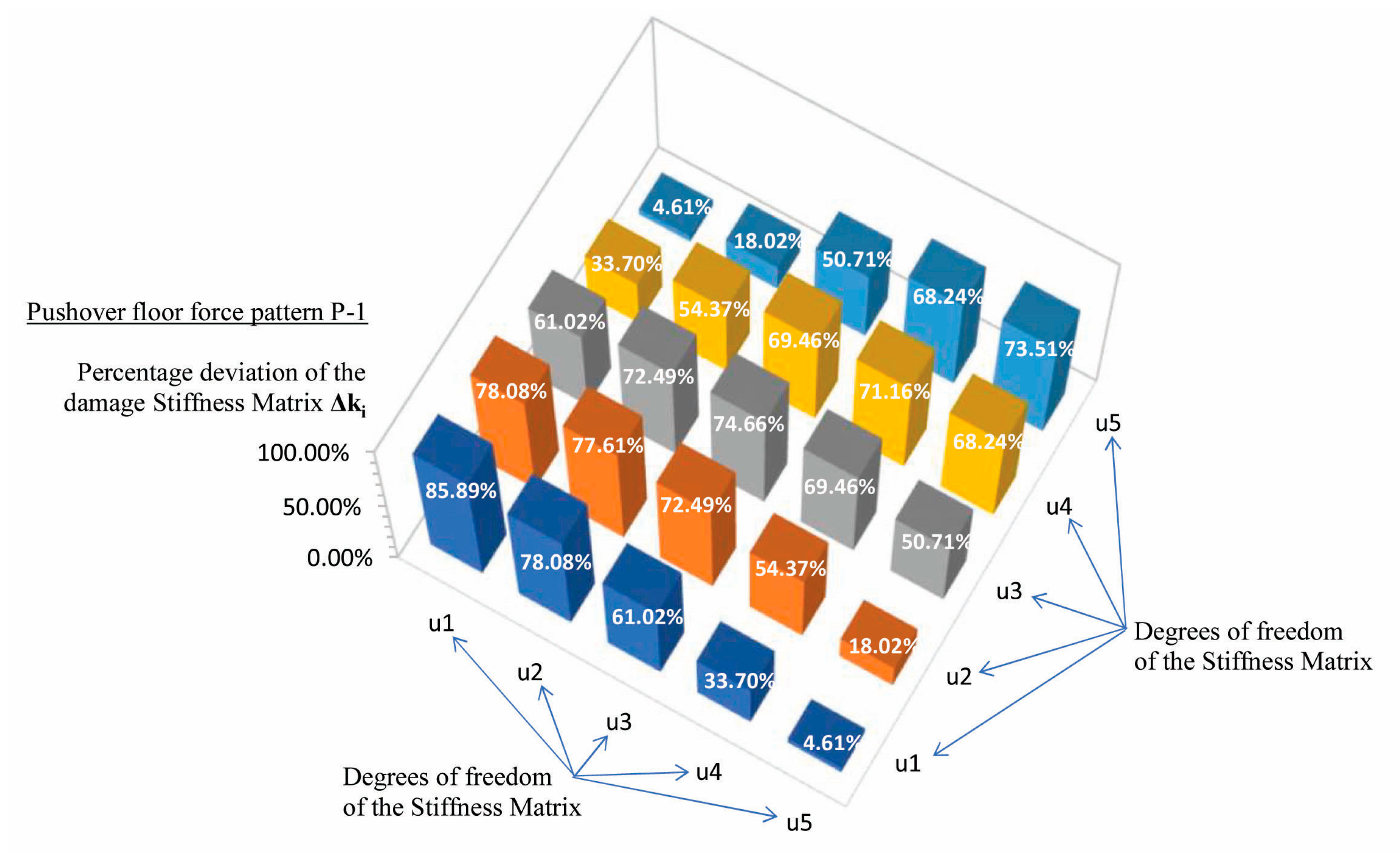
Figure 16. Percentage deviation of the Damage Stiffness matrix

{Δ k}_{i}

at the i-step (

θ_{p r} = 0.02 r a d

), for the triangular force pattern (P-1).

Figure 16. Percentage deviation of the Damage Stiffness matrix

{Δ k}_{i}

at the i-step (

θ_{p r} = 0.02 r a d

), for the triangular force pattern (P-1).

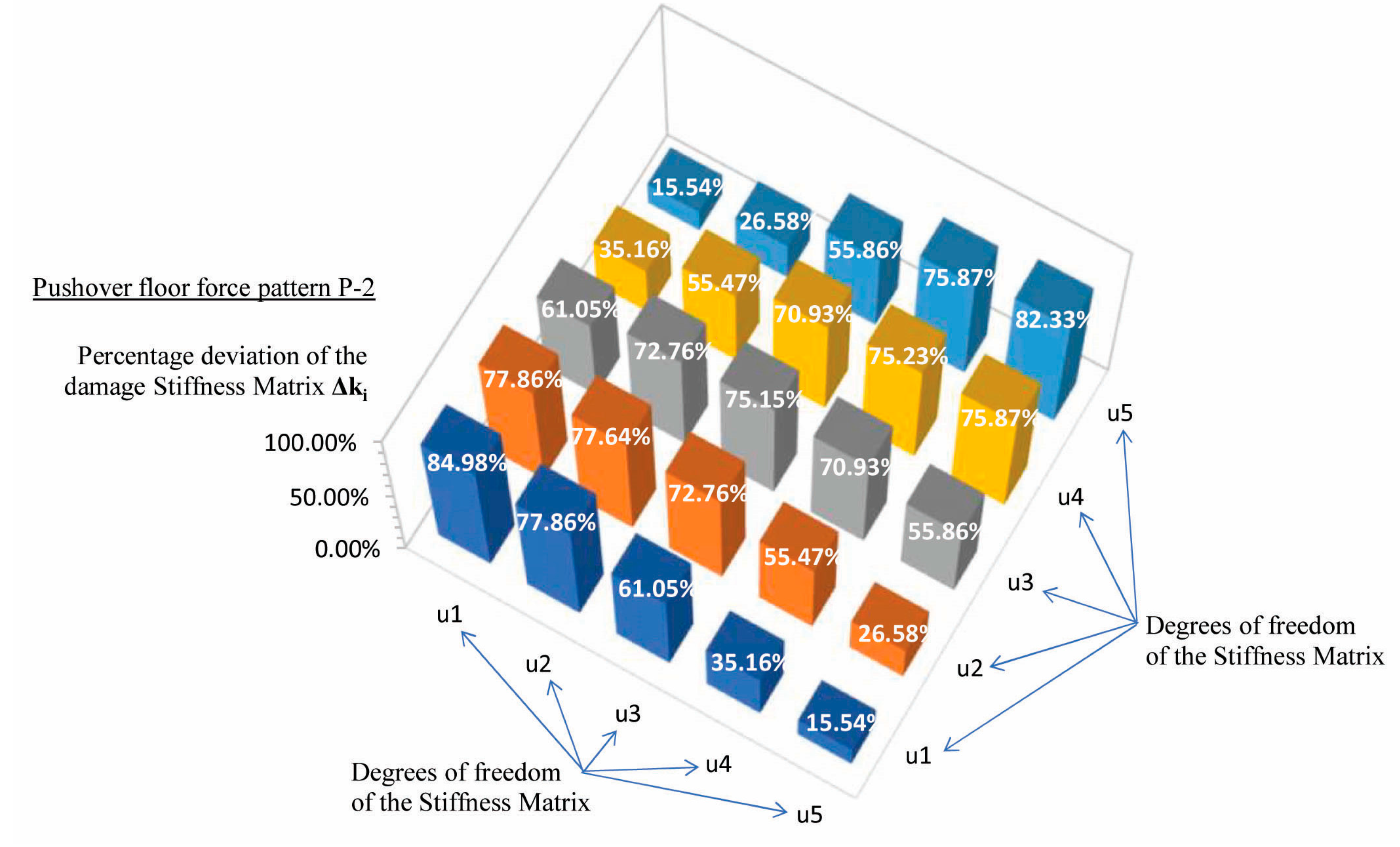
Figure 17. Percentage deviation of the Damage Stiffness matrix

{Δ k}_{i}

at the i-step (

θ_{p r} = 0.02 r a d

), for the triangular force pattern with an additional top force (P-2).

Figure 17. Percentage deviation of the Damage Stiffness matrix

{Δ k}_{i}

at the i-step (

θ_{p r} = 0.02 r a d

), for the triangular force pattern with an additional top force (P-2).

Table 1. Effective moment of inertia ratio (

I_{e f f} / I_{g}

) of RC structural elements as a function of the mean (chord) rotation of the frame structure

θ_{p r}

(rad).

Table 1. Effective moment of inertia ratio (

I_{e f f} / I_{g}

) of RC structural elements as a function of the mean (chord) rotation of the frame structure

θ_{p r}

(rad).

$θ_{p r}$	$I_{e f f} / I_{g}$	$θ_{p r}$	$I_{e f f} / I_{g}$	$θ_{p r}$	$I_{e f f} / I_{g}$	$θ_{p r}$	$I_{e f f} / I_{g}$
0.000	1.00	0.010	0.32	0.020	0.28	0.030	0.17
0.001	0.87	0.011	0.32	0.021	0.27	0.031	0.16
0.002	0.74	0.012	0.31	0.022	0.26	0.032	0.15
0.003	0.61	0.013	0.30	0.023	0.25	0.032+	Eq. (8)
0.004	0.50	0.014	0.30	0.024	0.24
0.005	0.43	0.015	0.30	0.025	0.23
0.006	0.40	0.016	0.30	0.026	0.22
0.007	0.37	0.017	0.29	0.027	0.21
0.008	0.35	0.018	0.29	0.028	0.19
0.009	0.34	0.019	0.28	0.029	0.18

Table 2. Percentage deviation of the Damage Stiffness matrix

{Δ k}_{i}

at the i-step (

θ_{p r} = 0.02 r a d

), for the triangular force pattern (P-1).

Table 2. Percentage deviation of the Damage Stiffness matrix

{Δ k}_{i}

at the i-step (

θ_{p r} = 0.02 r a d

), for the triangular force pattern (P-1).

Degrees offreedom	$u_{1}$	$u_{2}$	$u_{3}$	$u_{4}$	$u_{5}$
$u_{1}$	85.89%	78.08%	61.02%	33.70%	4.61%
$u_{2}$	78.08%	77.61%	72.49%	54.37%	18.02%
$u_{3}$	61.02%	72.49%	74.66%	69.46%	50.71%
$u_{4}$	33.70%	54.37%	69.46%	71.16%	68.24%
$u_{5}$	4.61%	18.02%	50.71%	68.24%	73.51%

Table 3. Percentage deviation of the Damage Stiffness matrix

{Δ k}_{i}

, at the i-step (

θ_{p r} = 0.02 r a d

), for the triangular force pattern with an additional top force (P-2).

Table 3. Percentage deviation of the Damage Stiffness matrix

{Δ k}_{i}

, at the i-step (

θ_{p r} = 0.02 r a d

), for the triangular force pattern with an additional top force (P-2).

Degrees offreedom	$u_{1}$	$u_{2}$	$u_{3}$	$u_{4}$	$u_{5}$
$u_{1}$	84.98%	77.86%	61.05%	35.16%	15.54%
$u_{2}$	77.86%	77.64%	72.76%	55.47%	26.58%
$u_{3}$	61.05%	72.76%	75.15%	70.93%	55.86%
$u_{4}$	35.16%	55.47%	70.93%	75.23%	75.87%
$u_{5}$	15.54%	26.58%	55.86%	75.87%	82.33%

Disclaimer/Publisher’s Note: The statements, opinions and data contained in all publications are solely those of the individual author(s) and contributor(s) and not of MDPI and/or the editor(s). MDPI and/or the editor(s) disclaim responsibility for any injury to people or property resulting from any ideas, methods, instructions or products referred to in the content.

© 2023 by the authors. Licensee MDPI, Basel, Switzerland. This article is an open access article distributed under the terms and conditions of the Creative Commons Attribution (CC BY) license (http://creativecommons.org/licenses/by/4.0/).

Copyright: This open access article is published under a Creative Commons CC BY 4.0 license, which permit the free download, distribution, and reuse, provided that the author and preprint are cited in any reuse.

MDPI Initiatives

Important Links

Choose an area of interest and we will send you notifications of new preprints at your preferred frequency.

Disclaimer

Identification of Damage in Planar Multi-Storey Reinforced Concrete Frames Developing a Beam-Sway Plastic Mechanism Using the “M and P” Technique

Abstract

1. Introduction

2. Materials and Methods

3. Numerical Example

4. Discussion

5. Conclusions

Author Contributions

Funding

Data Availability Statement

Conflicts of Interest

References

MDPI Initiatives

Important Links

Subscribe