Evaporation of Small Sessile Drop Deposited on Horizontal Solid Surface: New Exact Solutions and Approximations

Peter Lebedev-Stepanov; Olga Savenko

doi:10.20944/preprints202308.1274.v1

Preprint

Article

Evaporation of Small Sessile Drop Deposited on Horizontal Solid Surface: New Exact Solutions and Approximations

This version is not peer-reviewed.

Peter Lebedev-Stepanov^*

,Olga Savenko

Peter Lebedev-Stepanov^*

,Olga Savenko

This version is not peer-reviewed.

Downloads

112

Views

Comments

Submitted:

16 August 2023

Posted:

17 August 2023

You are already at the latest version

A peer-reviewed article of this preprint also exists.

Abstract

Evaporating liquid sessile drop deposited on horizontal surface is an important object of applications (printing technologies, electronics, sensorics, medical diagnostics, hydrophobic coatings, etc.) and theoretical investigations (microfluidics, self-assembly of nanoparticle, crystallization of the solute, etc.). The arsenal of formulas for calculating the slow evaporation of an axisymmetric drop of capillary dimensions deposited on a flat solid surface is reviewed. Such characteristics as vapor density, evaporation flux density, total evaporation rate are considered. Exact solutions obtained in the framework of the Maxwellian model, in which the evaporation process of the drop is limited by vapor diffusion from the drop surface to the surrounding air, are presented. The summary covers both well-known results obtained during the last decades and new results published by us in the last few years, but practically unknown to the wide scientific community. The newest formulas, not yet published in refereed publications, concerning exact solutions for a number of specific contact angles are also presented. In addition, new approximate solutions are presented for the first time (total evaporation rate and mass loss per unit surface area per unit time in the whole range of contact angles ), which can be used in modeling without requiring significant computational resources.

Keywords:

sessile liquid droplet

;

evaporation rate

;

diffusion

;

Laplace equation

;

analytical solution

;

flux density

;

mass loss per unit surface area per unit time

Subject:

Chemistry and Materials Science - Surfaces, Coatings and Films

1. Introduction

Evaporating liquid sessile drop is an important object both for theoretical investigations (evaporation dynamics, microfluidics, self-organization of solute, etc.) and wide variety of applications (printing technologies for functional coatings, medical diagnostics, food science, geophysics, etc.) [1,2,3,4,5,6,7,8,9,10].

The model of diffusion-limited quasi-stationary evaporation of the spherical droplet in quiescent air environment was originally proposed by J.C. Maxwell [11]. He calculated the diffusive drift of vapor from the surface of the evaporating droplet into the air, assuming that the vapor concentration at the surface of the droplet determines by saturated vapor density. This is valid for a drop radius much larger than the mean free path length of vapor molecules in the air. For example, this is not true for droplets smaller than 100 nm in the normal conditions.

Within the framework of the Maxwellian model (quasi-stationary evaporation), the diffusion equation practically turns into the Laplace equation for the vapor concentration,

\nabla^{2} n = 0

, with the following initial boundary conditions: on the drop surface

n (S) = n_{s}

. Outside the drop the vapor concentration is determined by the asymptotic value of the vapor concentration in the atmosphere (for aqueous solution, it is the relative humidity of the air,

n (\infty) = n_{\infty}

It is considered that the liquid-gas transition layer is infinitely thin compared to the droplet size. Moreover, for correctness of the Maxwellian model it is necessary to assume that density of air is much greater than vapor density, so that diffusion of vapor is determined by the vapor diffusion coefficient in the air. In particular, this requirement means that we must consider liquid at a temperature much smaller than its boiling point at a given air pressure.

The smallness of the convective Stefan flux also has to be satisfied. Stephan showed for the first time [12] that near the surface of an evaporating drop there is an air current directed away from the surface, because in order to maintain the constancy of the total pressure in the medium under conditions of vapor production by the liquid surface, along with the gradient of the vapor density there must exist an equal and opposite in direction gradient of the partial pressure of the other components of the air.

Fuchs showed [13] that the relative contribution of the Stefan flux to the evaporation process is given by factor

\frac{p_{s} + p_{\infty}}{2 p}

, where p is the pressure of the air,

p_{s}

and

p_{\infty}

are the saturated vapor pressure and the vapor pressure in the air far from the droplet, respectively. That factor for a drop of water under normal conditions does not exceed 1-2 percents (%). This is one of essential limitations of the Maxwellian model accuracy that indicates acceptable correctness of approximate solutions with respect to exact solutions of the diffusion problem. There are also other error factors: inaccurate determination of such parameters as drop surface temperature, vapor diffusion coefficient in air at a given temperature, saturated vapor pressure, etc. The capillary surface oscillations, air movement near the drop surface also are the factors that introduce uncertainties. Therefore, the approximate solutions whose accuracy is of the order of 5 percents can be considered acceptable.

In the following, we consider the small drop deposited on a flat solid horizontal substrate (so-called sessile drop). It is easy to derive that the equilibrium shape of a sessile drop of a slowly evaporating liquid, the size of which is much smaller than the capillary constant (Bond number, Bo<<1), approximately corresponds to a spherical segment with the given contact (wetting) angle. Sessile water droplets with a height of less than 1 mm satisfy this criterion quite well.

The Maxwellian model was apparently first applied to such sessile drop in the paper of Picknett and Bexon [14]. All solutions described below in this paper are given within the framework of this approach.

Exact analytical solutions have been obtained to describe the total evaporation rate (mass loss per unit time) and evaporation flux density (mass loss per unit surface area per unit time) of a small sessile liquid droplet having the shape of an axisymmetric spherical segment deposited on a horizontal substrate [15,16,17,18,19,20,21,22,23,24].

There are currently two alternative expressions for the droplet evaporation flux density that are mathematically equivalent. First, the following solution was proposed [19,20]

\begin{array}{l} J (α) = D \frac{n_{s} - n_{\infty}}{R} \times \\ \times [\frac{\sin θ}{2} + \sqrt{2} {(\cosh α + \cos θ)}^{3 / 2} \int_{0}^{\infty} \frac{\cosh θ τ}{\cosh π τ} \tanh [(π - θ) τ] P_{- 1 / 2 + i τ} (\cosh α) τ d τ], \end{array}

(1)

where

is the Legendre function of the first kind. Here, toroidal coordinate

α

ranges in the interval from 0 (top of the drop) to ∞ (contact line). So, this coordinate is related to the cylindrical coordinate r by

r = \frac{R \sinh α}{\cosh α + \cos θ}

(2)

where

θ

is the contact angle of the droplet (Figure 1). Equation (1) is a double integral, being an implicit function of cylindrical coordinate r, which makes formula (1) extremely difficult to use in calculations. A simpler from a computational point of view, but mathematically equivalent expression in polar coordinates was also obtained [21,22]. It allows to calculate the flux density at the surface of the droplet as a function of the polar angle φ explicitly (Figure 1):

J (φ) = \frac{D (n_{S} - n_{\infty})}{R} f (φ)

(3)

where

f (φ) = \frac{π}{{(π - θ)}^{2}} \frac{\sin^{3} θ}{\cos φ - \cos θ} \int_{φ}^{θ} \frac{{(1 - \cos (θ + β))}^{\frac{π}{2 (π - θ)}} - {(1 - \cos (θ - β))}^{\frac{π}{2 (π - θ)}}}{{({(1 - \cos (θ + β))}^{\frac{π}{2 (π - θ)}} + {(1 - \cos (θ - β))}^{\frac{π}{2 (π - θ)}})}^{2}} \frac{{(\cos β - \cos θ)}^{\frac{π}{2 (π - θ)} - \frac{1}{2}} d β}{\sqrt{\cos φ - \cos β}} .

(4)

Unfortunately, unlike expression (1), equations (3)-(4) are not yet known to the wider community and are completely ignored in the latest topical review [23].

For the total evaporation rate, the following expression was obtained [20]:

W (θ) = π R D (n_{s} - n_{\infty}) [\frac{\sin θ}{1 + \cos θ} + 4 \int_{0}^{\infty} \frac{1 + \cosh 2 θ τ}{\sinh 2 π τ} \tanh [(π - θ) τ] d τ]

(5)

where D is a diffusion coefficient of the vapor in the air, n is a vapor volume concentration outside the drop with the boundary conditions n = n_s at the drop air-liquid surface and far from the drop, R is the radius of contact line. However, as shown in [22], although the formula (5), correctly describes almost the entire dependence

W (θ)

, where

θ \in [0, π)

, it gives wrong result in the limit at

θ = π

, which can be determined by the direct calculation.

From the point of view of application in computer simulations, this universal analytical expression that describes the evaporation flux density over the entire range of contact angles 0– π (0–180 degrees), is still quite complex. It requires significant computational resources. To accelerate the calculations of the evaporation flux density, it is reasonable to use simplified approximate expressions.

For example, there is a very good approximation for the integral evaporation flux proposed by Picknett and Bexon [14]:

W (θ) = 2 π ρ D (n_{s} - n_{\infty}) g (θ)

(6)

where

\begin{array}{l} g (θ) = 0.6366 θ + 0.09591 θ^{2} - 0.06144 θ^{3}, 0 \leq θ \leq 0.175; \\ g (θ) = 0.00008957 + 0.6333 θ + 0.1160 θ^{2} - 0.08878 θ^{3} + 0.01033 θ^{4}, 0.175 \leq θ \leq π . \end{array}

(7)

This expression has a maximum error of about 0.2% and looks much more preferable for simulation than the exact analytical solution (5). In Section 3 of this paper, we propose a much simpler approximate solution in place of equations (6)-(7) and apply it to calculate the droplet evaporation time under different contact line motion scenarios.

Similarly, for the evaporation flux density, instead of the exact formulas (1) or (3), approximate expressions can be proposed for selected narrow ranges of droplet contact angles. So, earlier an expression for the evaporation flux density was proposed, applicable in the case of small contact angles [24]:

J (r) = J_{0} (θ) {(1 - \frac{r^{2}}{R^{2}})}^{- λ (θ)}, λ (θ) = \frac{1}{2} - \frac{θ}{π},

(8)

where

J_{0} (θ) = \frac{D (n_{s} - n_{\infty})}{R} (0.27 θ^{2} + 1.30) (0.6381 - 0.2239 {(θ - 0.25 π)}^{2})

Equation (8), being represented in the form of equations (3)-(4), can be rewritten as

​ J (φ) = \frac{D (n_{s} - n_{\infty})}{R} \overset{⌣}{f} (φ)

(9)

where

\overset{⌣}{f} (φ) = {(1 - \frac{\sin^{2} φ}{\sin^{2} θ})}^{- λ (θ)} (0.27 θ^{2} + 1.30) (0.6381 - 0.2239 {(θ - 0.25 π)}^{2})

(10)

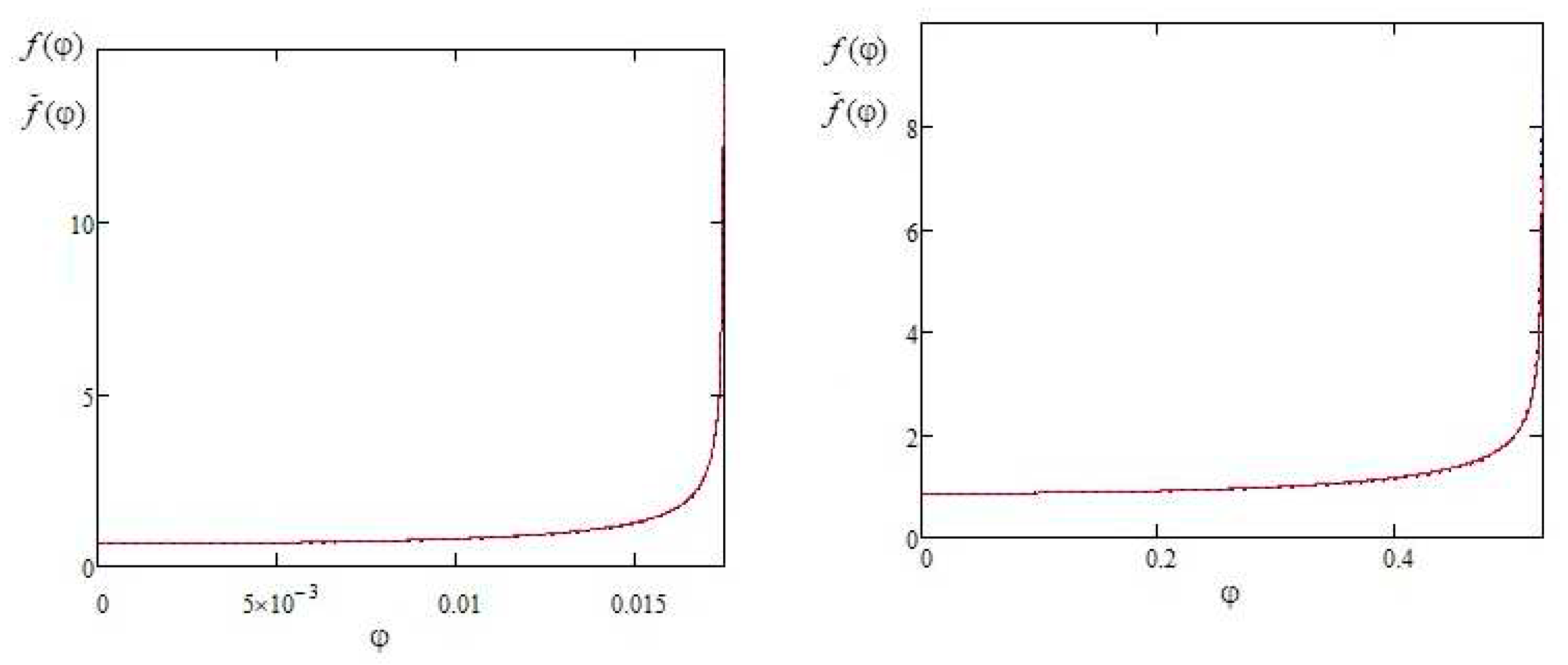
This expression gives a quite good description for contact angles smaller than 30 degrees (π/6). The graph that is represented in Figure 2 shows a comparison of the approximate expression (10) with the exact solution (3) for the contact angles of 1 degree and 30 degrees.

It can be seen from the comparison that the error of the approximate expression (10) increases as angle φ approaches θ. Except for the region of φ angles near θ, the deviation of the approximate formula (10) from the exact solution (4) practically does not exceed 2%, which makes formula (10) suitable for describing droplets with sharp contact angles in the range approximately 0-30 degrees.

However, the question of which simplified formulas would be appropriate to apply in other ranges of contact angles, for example, in the case of water drop deposited on hydrophobic substrates, still remains open. In Section 3 of this paper, we propose an approximate variant of exact expressions (3)- (4) in the whole range of contact angles

θ \in [0, ​ ​ ​ π)

) that answers this question.

2. New exact solutions for some values of contact angles

Previously [21,22], an expression was obtained that describes the vapor concentration near an evaporating drop:

\begin{array}{l} n (ω, ξ) = n_{S} - \frac{2 (n_{S} - n_{\infty})}{π - θ} {(\cosh ω - \cos ξ)}^{1 / 2} \cos \frac{π ξ}{2 (π - θ)} \times \\ \times \int_{ς = ω}^{\infty} {(\cosh \frac{π ς}{(π - θ)} - \cos \frac{π ξ}{(π - θ)})}^{- 1} \frac{\sinh \frac{π ς}{2 (π - θ)} d ς}{\sqrt{\cosh ς - \cosh ω}} \end{array}

(11)

This expression can also be represented as:

\begin{array}{l} n (ω, ξ) = n_{s} - \frac{(n_{s} - n_{\infty})}{2 γ} {(\cosh ω - \cos ξ)}^{1 / 2} \times \\ \times \int_{ω}^{\infty} [\frac{\sinh \frac{π ς}{2 γ}}{\cosh \frac{π ς}{2 γ} - \cos \frac{π ξ}{2 γ}} - \frac{\sinh \frac{π ς}{2 γ}}{\cosh \frac{π ς}{2 γ} + \cos \frac{π ξ}{2 γ}}] \frac{d ς}{\sqrt{\cosh ς - \cosh ω}} . \end{array}

(11a)

Here

γ = π - θ

. Integral (11a) can be represented as the sum of a finite number of terms for some specific contact angles [25,26]. It was shown that expression (11a) under the condition

ξ = \frac{π}{2 j}, where j = 1, 2, 3, \dots

(12)

can be rewritten as

\begin{array}{l} n (ω, ξ) = n_{s} - (n_{s} - n_{\infty}) {(\cosh ω - \cos ξ)}^{1 / 2} \times \\ \times \sum_{k = 0}^{k = j - 1} {\frac{1}{\sqrt{\cosh ω - \cos [ξ + 2 k π j^{- 1}]}} - \frac{1}{\sqrt{\cosh ω - \cos [ξ + (2 k - 1) π j^{- 1}]}}} \end{array}

(13)

Then, evaporation flux density is given by [21,22]

J = - D \frac{\cosh ω - \cos ξ}{R} \frac{\partial n (ω, ξ)}{\partial ξ} = \frac{(n_{s} - n_{\infty}) D}{R} (\cosh ω - \cos ξ) \frac{\partial ψ (ω, ξ)}{\partial ξ}

(14)

where

\begin{array}{l} ψ (ω, ξ) = {(\cosh ω - \cos ξ)}^{1 / 2} \times \\ \times \sum_{k = 0}^{k = j - 1} {\frac{1}{\sqrt{\cosh ω - \cos [ξ + 2 k π j^{- 1}]}} - \frac{1}{\sqrt{\cosh ω - \cos [ξ + (2 k - 1) π j^{- 1}]}}} \end{array}

By differentiating in the formula (13), we get

J = \frac{(n_{s} - n_{\infty}) D}{R} \tilde{J}

(15)

where

\begin{array}{l} \tilde{J} = {(\cosh ω - \cos ξ)}^{1 / 2} \frac{\sin (0.5 π j^{- 1})}{2} \times \\ \times \sum_{k = 0}^{k = j - 1} {\frac{1}{\sqrt{\cosh ω - \cos [ξ + 2 k π j^{- 1}]}} - \frac{1}{\sqrt{\cosh ω - \cos [ξ + (2 k - 1) π j^{- 1}]}}} - \\ - \frac{{(\cosh ω - \cos ξ)}^{3 / 2}}{2} \times \\ \times \sum_{k = 0}^{k = j - 1} {\frac{\sin [ξ + 2 k π j^{- 1}]}{{(\cosh ω - \cos [ξ + 2 k π j^{- 1}])}^{\frac{3}{2}}} - \frac{\sin [ξ + (2 k - 1) π j^{- 1}]}{{(\cosh ω - \cos [ξ + (2 k - 1) π j^{- 1}])}^{\frac{3}{2}}}} \end{array}

(16)

It can be shown that the first sum in formula (16) gives identically zero (can be verified by direct calculation), and the terms in brackets in the second sum are equal in absolute value. With this in mind, the expression is greatly simplified

\tilde{J} = {(\cosh ω - \cos ξ)}^{3 / 2} \sum_{k = 0}^{k = j - 1} \frac{\sin [ξ + 2 k π j^{- 1}]}{{(\cosh ω - \cos [ξ + 2 k π j^{- 1}])}^{\frac{3}{2}}}

(17)

Taking into account (11), we get

\tilde{J} (j) = {(\cosh ω - \cos 0.5 π j^{- 1})}^{3 / 2} \sum_{k = 0}^{k = j - 1} \frac{\sin [0.5 π j^{- 1} + 2 k π j^{- 1}]}{{(\cosh ω - \cos [0.5 π j^{- 1} + 2 k π j^{- 1}])}^{\frac{3}{2}}}

(18)

Thus, for any j, the evaporation flux density is given by [25]

J (j) = \frac{(n_{s} - n_{\infty}) D}{R} {(\cosh ω - \cos 0.5 π j^{- 1})}^{3 / 2} \sum_{k = 0}^{k = j - 1} \frac{\sin [0.5 π j^{- 1} + 2 k π j^{- 1}]}{{(\cosh ω - \cos [0.5 π j^{- 1} + 2 k π j^{- 1}])}^{\frac{3}{2}}}

(19)

If k=j, the term under summation in (19) has the form

\frac{\sin [0.5 π j^{- 1} + 2 j π j^{- 1}]}{{(\cosh ω - \cos [0.5 π j^{- 1} + 2 j π j^{- 1}])}^{\frac{3}{2}}} = \frac{\sin [0.5 π j^{- 1}]}{{(\cosh ω - \cos [0.5 π j^{- 1}])}^{\frac{3}{2}}}

(20)

If k=0, the term under summation in (19) has the same form

\frac{\sin [0.5 π j^{- 1}]}{{(\cosh ω - \cos [0.5 π j^{- 1}])}^{\frac{3}{2}}} = \frac{\sin [0.5 π j^{- 1}]}{{(\cosh ω - \cos [0.5 π j^{- 1}])}^{\frac{3}{2}}}

(21)

Taking into account (20) and (21), equation (19) can be transformed as

J (j) = \frac{(n_{s} - n_{\infty}) D}{R} {(\cosh ω - \cos 0.5 π j^{- 1})}^{3 / 2} \sum_{k = 1}^{k = j} \frac{\sin [0.5 π j^{- 1} + 2 k π j^{- 1}]}{{(\cosh ω - \cos [0.5 π j^{- 1} + 2 k π j^{- 1}])}^{\frac{3}{2}}}

(22)

Expression (22) is the equivalent to (19).

To apply expressions (19) or (22) for calculations, it is necessary to take into account the formula (11) and following geometric relationship [21,22]:

\cosh ω = \frac{\sin^{2} ξ}{\cos φ + \cos ξ} + \cos ξ

(23)

To establish a relationship between the parameter j and the corresponding contact angle

θ

, one has to use the geometric relation

ξ = π - θ

(24)

It means that

θ = π (1 - \frac{1}{2 j}) = π \frac{2 j - 1}{2 j}, where j = 1, 2, 3, \dots

(25)

Table 1 shows the first two solutions corresponding to j=1, 2, 3. It's obvious that

\lim_{j \to \infty} θ = π

(26)

First three solution of the expression (22) with j=1,2,3 are placed into Table 1. These mean that the general solution

f (θ)

given by equation (4) can be represented as:

f_{θ = 90^{o}} (φ) = 1

(27)

f_{θ = 135^{o}} (φ) = \frac{1}{\sqrt{2}} - \frac{0.25}{{(\frac{3}{2} + \sqrt{2} \cos φ)}^{\frac{3}{2}}}

(28)

f_{θ = 150^{o}} (φ) = \frac{1}{2} (1 + {(7 + 4 \sqrt{3} \cos φ)}^{- \frac{3}{2}} - 2 {(4 + 2 \sqrt{3} \cos φ)}^{- \frac{3}{2}})

(29)

Figure 3 represents the dependences of the evaporation flux density (dimensionless) on the polar angle, which is given by formulas (28) and (29).

It is easy to verify by direct calculation that formula (4) gives the same curves, which confirms the correctness of the mathematical transformation that led to the formula (19) or the expression (22).

3. New approximate solutions

3.1. Total evaporation rate

Let us consider compact approximate expression for the total evaporation rate of the form

\overset{⌣}{W} (θ) = 4 (\ln 2) π ρ D (n_{s} - n_{\infty}) \sin \frac{θ}{2}

(30)

and compare formula (30) with the very accurate approximation of Picknett and Bexon (6). For this purpose, one can represent equation (30) in the form (6):

\overset{⌣}{W} (θ) = 2 π ρ D (n_{s} - n_{\infty}) \overset{⌣}{g} (θ)

(31)

where

\overset{⌣}{g} (θ) = 2 \ln 2 \sin \frac{θ}{2}

(32)

Figure 4 shows a graph of the function

\overset{⌣}{g} (θ)

together with the exact solution

g (θ)

. We see that visually the approximate solution (30) practically does not differ from the exact one. The maximum relative error reaches 9 percent, and the average error over the entire contact angle change interval, calculated by the formula

\frac{1}{π} \int_{0}^{π} \frac{\overset{⌣}{g} (x) - g (x)}{g (x)} d x \cdot 100 \frac{0}{0}

(33)

does not exceed 1.5 percent (%).

Formula (30) can be recommended for estimating drop evaporation time if its contact angle varies over a wide range during evaporation. For example, this scenario occurs when a drop of aqueous solution evaporates on a hydrophobic substrate under contact line pinning conditions. Theoretically, equation (30) allows us to calculate the evaporation time of a sessile droplet at any character of dependence of the droplet radius on the contact angle during evaporation. Two extreme scenarios of contact line behavior are distinguished: the constant contact line radius mode (CCR) and the constant contact angle mode (CCA) [14].

The change in volume of a drop for time dt is defined by

d V = - W (θ) n_{L}^{- 1} d t

(34)

where

n_{L}

is volume concentration of evaporating molecules in the liquid. The volume of the droplet with contact angle θ and spherical segment radius ρ (Figure 1) is determined by

V = π ρ^{3} (\frac{2}{3} - \cos θ + \frac{\cos^{3} θ}{3})

(35)

Substituting equations (30) and (35) into expression (34), one can obtain the differential equation

π \frac{d}{d t} ρ^{3} (\frac{2}{3} - \cos θ + \frac{\cos^{3} θ}{3}) = - 4 π ρ D (n_{s} - n_{\infty}) n_{L}^{- 1} \ln 2 \sin \frac{θ}{2}

(36)

which allows to calculate the rate of drop size change under any scenario of contact line motion

θ (t)

. In particular, the condition that is satisfied in the CCR mode can be written as follows

R = ρ \sin θ = const

(37)

In that case

d V = \frac{π R^{3} d θ}{{(1 + c o s θ)}^{2}}

By expressing

ρ

from equation (37), substituting it into (36), and performing trigonometric transformations, we get the evaporating time of the droplet of radius R and contact angle θ for CCR mode

t = \frac{n_{L} R^{2}}{4 \ln 2 (n_{s} - n_{\infty}) D} \int_{0}^{\frac{θ}{2}} \frac{d ξ}{\cos^{3} ξ}

(38)

t = \frac{n_{L} R^{2}}{8 \ln 2 (n_{s} - n_{\infty}) D} [\frac{\sin \frac{θ}{2}}{\cos^{2} \frac{θ}{2}} + \ln (\tan (\frac{π + θ}{4}))], θ \in [0, ​ ​ ​ π)

(39)

If we consider a drop of aqueous solution on a hydrophobic surface with an initial contact angle close to π, then its dimensions are conveniently characterized by the radius of the spherical segment and the contact angle at the initial instant of time. Then formula (39) can be conveniently rewritten as

t_{C C R} = \frac{n_{L} ρ^{2} \sin^{2} θ}{8 \ln 2 (n_{s} - n_{\infty}) D} [\frac{\sin \frac{θ}{2}}{\cos^{2} \frac{θ}{2}} + \ln (\tan (\frac{π + θ}{4}))], θ \in [0, ​ ​ ​ π), ρ \sin θ = const .

(40)

Since, as follows from equation (35), the segment radius is described by the formula

ρ = V^{\frac{1}{3}} π^{- \frac{1}{3}} {(\frac{2}{3} - \cos θ + \frac{\cos^{3} θ}{3})}^{- \frac{1}{3}}

then expression (40) can be rewritten as

t_{C C R} = \frac{n_{L} V^{\frac{2}{3}} \sin^{2} θ}{8 π^{\frac{2}{3}} \ln 2 (n_{s} - n_{\infty}) D} [\frac{\sin \frac{θ}{2}}{\cos^{2} \frac{θ}{2}} + \ln (\tan (\frac{π + θ}{4}))] {(\frac{2}{3} - \cos θ + \frac{\cos^{3} θ}{3})}^{- \frac{2}{3}}

(40a)

Similarly, for the evaporation time of a drop in the CCA mode one can obtain

t_{C C A} = \frac{3 V^{\frac{2}{3}} n_{L}}{8 π^{\frac{2}{3}} \ln 2 D (n_{s} - n_{0}) \sin \frac{θ}{2}} {(\frac{2}{3} - \cos θ + \frac{\cos^{3} θ}{3})}^{\frac{1}{3}}, θ = const .

(41)

Let's look at a practical example [27]: we have the water droplet with initial volume 1 μL , and initial θ = 110 deg, vapor diffusion coefficient, D = 25.41 × 10⁻⁶ m²/s, saturated vapor concentration n_s = 0.0175 kg/m3, relative humidity (H)= 0.29. Calculations according to formulas (40a) and (40) give the following values:

t_{C C R} = 860 s

and

t_{C C A} = 974 s

. Figure 5 shows the graphs of the evaporation time of a drop with the indicated parameters as a function of the initial volume parameter in both modes. We see that at equal initial volumes and initial contact angles, evaporation in the CCR mode is faster than in the CCA mode, as it should be, based on the general ideas about evaporation.

The authors of the paper [27] calculated the evaporation time in this case on the basis of the Popov model [20], i.e., using the equation (5). They obtained the following values:

t_{C C R} = 870 s

and

t_{C C A} = 954 s

. We see that these values are insignificantly different from the values obtained by the formulas (40a) and (41). At the same time, as indicated in the paper [26], the experiment that was made for such a drop drying in the CCA mode gives the evaporation time of 1009 s. We can conclude that, with respect to the real experiment, the simplified formula (30) gives approximately the same error as the complex expression (5).

3.1. Evaporation flux density for acute and obtuse contact angles

The previously derived new expression for the evaporation flux density gives new possibilities for finding approximate relations. Let us consider the expression for the evaporation flux density in bipolar coordinates [21,22]:

J (ω) = \frac{π D (n_{S} - n_{\infty})}{2 {(π - θ)}^{2} R} {(\cosh ω - \cos (π - θ))}^{3 / 2} \int_{ω}^{\infty} \frac{\sinh \frac{π ς}{2 (π - θ)}}{\cosh^{2} \frac{π ς}{2 (π - θ)}} \frac{d ς}{\sqrt{\cosh ς - \cosh ω}}

(42)

where

\cosh ω

is determined by the equation (23).

Obviously, for obtuse contact angles, the value of

(π - θ)

is small. In this case, the argument of hyperbolic functions containing

(π - θ)

in the denominator under the integral will be large, so that

\tanh \frac{π ς}{2 (π - θ)} \to 1

. Consequently, the asymptotics of expression (42) is determined by

\cosh^{- 1} \frac{π ω}{2 (π - θ)}

. Therefore, taking into account equation (23), the asymptotic expression can be written as follows

J (φ) \propto \frac{\cosh^{- 1} \frac{π ω (φ)}{2 (π - θ)}}{\cos φ - \cos θ}

(43)

where

ω (φ) = arc \cosh [\frac{1 - \cos φ \cos θ}{\cos φ - \cos θ}]

(44)

Taking into account (23), one can obtain

\sinh ω = \frac{\sin φ \sin θ}{\cos φ - \cos θ}

(45)

Performing the transformations, we have

\cosh \frac{π ω (φ)}{2 (π - θ)} = \frac{1}{2} {[\frac{1 - \cos (φ + θ)}{\cos φ - \cos θ}]}^{\frac{π}{2 (π - θ)}} + \frac{1}{2} {[\frac{1 - \cos (φ - θ)}{\cos φ - \cos θ}]}^{\frac{π}{2 (π - θ)}}

(46)

Substituting equation (46) into (43), one can obtain

J (φ) \propto \frac{2 {[\cos φ - \cos θ]}^{\frac{π}{2 (π - θ)} - 1}}{{[1 - \cos (φ + θ)]}^{\frac{π}{2 (π - θ)}} + {[1 - \cos (φ - θ)]}^{\frac{π}{2 (π - θ)}}}

(47)

Comparing formula (43) with expressions (3)-(4), taking into account (47), let us write an approximate expression for function (4) in the following form

\overset{⌣}{f} (φ) = \frac{π \sin^{3} θ}{{(π - θ)}^{2} \sin \frac{θ}{2}} \frac{{[\cos φ - \cos θ]}^{\frac{π}{2 (π - θ)} - 1} \times P (θ)}{{[1 - \cos (φ + θ)]}^{\frac{π}{2 (π - θ)}} + {[1 - \cos (φ - θ)]}^{\frac{π}{2 (π - θ)}}}

(48)

where

P (θ)

is correction factor that, in general, depends on the contact angle.

Our studies have shown that, in the first approximation, to obtain a relatively good description of the evaporation flux density in the whole range of contact angles

θ \in [0, ​ ​ ​ π)

using formula (48), it is convenient to choose a correction factor in the form of a constant

P \approx 1.166

(49)

Taking into account (49), expression (48) can be rewritten as

\overset{⌣}{f} (φ) = \frac{1.166 π \sin^{3} θ}{{(π - θ)}^{2} \sin \frac{θ}{2}} \frac{{[\cos φ - \cos θ]}^{\frac{π}{2 (π - θ)} - 1}}{{[1 - \cos (φ + θ)]}^{\frac{π}{2 (π - θ)}} + {[1 - \cos (φ - θ)]}^{\frac{π}{2 (π - θ)}}}

(50)

Evaporation flux density can be calculated by a formula similar to equation (3):

J (φ) = \frac{D (n_{S} - n_{\infty})}{R} \overset{⌣}{f} (φ)

(51)

Figure 6 represents the calculation results of the dimensionless evaporation flux density, determined by the approximate formula (50), together with the exact solution, determined by expression (4), for some acute and obtuse contact angles of a sessile droplet.

In general, Figure 6 shows that the approximate formula (50) can adequately describe the behavior of the evaporation flux density over the entire range of contact angles

θ \in [0, ​ ​ ​ π)

, more accurately for acute angles than for obtuse angles. A more detailed approach requires breaking the entire range of contact angles into smaller sub-intervals and finding correction functions

P (θ)

for each sub-interval, possibly in a polynomial representation. This procedure is beyond the scope of this publication.

4. Discussion

The arsenal of formulas for calculating the slow evaporation of an axisymmetric drop of capillary dimensions deposited on a flat solid surface is reviewed. Such characteristics as vapor density, evaporation flux density, total evaporation rate are considered. Exact solutions obtained in the framework of the Maxwellian model, in which the evaporation process of the drop is limited by vapor diffusion from the drop surface to the surrounding air, are presented.

Along with the long-known solutions published by Popov et al. [19,20] during the last two decades, the existence of alternative expression to describe evaporation flux density is pointed out. This alternative equation depends explicitly on the polar angle and is a one-dimensional integral (3)-(4), while the corresponding mathematical equivalent expression of Popov et al. (1) is a double integral with implicit dependence on the cylindrical coordinate. We draw the attention of researchers to the paper [22], which, apparently, remained unknown to the authors of the newest review of Wilson and D’Ambrosio [23] on drop evaporation.

New complex solution (22) was derived for the evaporation flux density of a small liquid droplet having the shape of an axisymmetric spherical segment deposited on a horizontal substrate for the set of discrete contact angles

θ = π (1 - \frac{1}{2 j})

, where j=1,2,3… As an example, very simple exact expressions (28) and (29) were obtained explicitly for the evaporation flux density for droplets with contact angles

\frac{3 π}{4} = 135

deg and

\frac{5 π}{6} = 150

deg that do not contain integral function. They can also be used as approximate expressions for a narrow range of contact angles around the specified values.

Also, new approximate solutions are presented for the first time: equation (30) - total evaporation rate and expression (50) - mass loss per unit surface area per unit time in the whole range of contact angles

θ \in [0, ​ ​ ​ π)

). These expressions are described through elementary functions and do not contain integrals. Thus, they can be used in modeling without requiring significant computational resources.

Expression (50), taking into account (48), contains significant potential for successive improvements in accuracy through the breakdown of the contact angle determination domain into intervals and the introduction of individual correction factors. That may be a further task to advance work in this direction.

Author Contributions

Conceptualization, methodology, derivation of the equations, writing, P. Lebedev-Stepanov; calculations and visualization, Olga Savenko. All authors have read and agreed to the published version of the manuscript.

Funding

This work was performed within the State assignment of Federal Scientific Research Center "Crystallography and Photonics" of Russian Academy of Sciences.

Institutional Review Board Statement

Not applicable.

Informed Consent Statement

Not applicable.

Data Availability Statement

Not applicable.

Conflicts of Interest

Author declares no conflict of interest.

References

Brutin, D. Droplet Wetting and Evaporation; Elsevier Inc: Amsterdam, Netherlands, 2015. [Google Scholar]
Zang, D., Tarafdar, S., Tarasevich, Yu.Yu., Choudhury, M.D., Dutta, T. Evaporation of a droplet: from physics to applications. Phys. Rep. 2019, 804, 1–56. [CrossRef]
Lebedev-Stepanov P., Vlasov, K. Simulation of self-assembly in an evaporating droplet of colloidal solution by dissipative particle dynamics. Coll. and Surf. A: Physicochem. Eng. Aspects 2013, 432, 132–138. [CrossRef]
Kolegov, K., Barash, L. Applying droplets and films in evaporative lithography. Adv. Colloid and Interface Sci. 2020, 285, 102271. [CrossRef] [PubMed]
Schnall-Levin, M., Lauga, E., Brenner, M.P. Self-assembly of spherical particles on an evaporating sessile droplet. Langmuir 2006, 22, 4547. [CrossRef] [PubMed]
Kokornaczyk, M.O., Bodrova, N.B., Baumgartner, S. Diagnostic tests based on pattern formation in drying body fluids—a mapping review. Colloids Surf. B: Biointerfaces. 2021, 208, 112092–1. [CrossRef] [PubMed]
Hamadeh, L., Imran, S., Bencsik, M., Sharpe, G.R., Johnson, M.A., Fairhurst, D.,J. Machine learning analysis for quantitative discrimination of dried blood droplets. Sci. Rep 2020, 10, 3313–3326. [CrossRef] [PubMed]
Lebedev-Stepanov, P.V., Buzoverya, M.E., Vlasov, K.O., Potekhina, Yu.P. Morphological analysis of images of dried droplets of saliva for determination the degree of endogenous intoxication. J. of Bioinformatics and Genomics 2018, 4, 1–4.
Boinovich, L.B., Emelyanenko, A.M. Hydrophobic materials and coatings: principles of design, properties and applications. Russ. Chem. Rev. 2008, 77, 583–600. [CrossRef]
Lebedev-Stepanov, P.V. Introduction to self-organization and self-assembly of ensembles of nanoparticles. NRNU MEPhI: Moscow, Russia, 2015 [in Russian].
Maxwell, J.C. Diffusion. In Collected Scientific Papers, Niven, W.D., Ed. Cambridge University Press: Cambridge, UK, 2010, Vol. 2, 625-646.
Stefan, J. Über die dynamische Theorie der Diffusion der Gase. Sitzungsberichte Akad Wiss 1872, 65, 323–363. [Google Scholar]
Fuchs, N.A. Evaporation and Droplet Growth in Gaseous Media. Pergamon Press: London, UK, 2013; pp.1-80.
Picknett, R.G., Bexon, R. The evaporation of sessile or pendant drops in still air. J. Colloid Interface Sci. 1977, 61, 336. [CrossRef]
Talbot, E., C., De Dier, R., Sempels, W., Vermant, J. Droplets Drying on Surfaces. In Fundamentals of Inkjet Printing; Hoath, S.D. (Ed.) Wiley-VCH Verlag GmbH & Co: Weinheim, Germany, 2016; pp. 251–279. [Google Scholar]
Wilson, S.K., Duffy, B.R. Mathematical Models for the Evaporation of Sessile Droplets. In Drying of Complex Fluid Drops; Brutin, D.; Sefiane, K. (Eds.) The Royal Society of Chemistry: Croydon, UK, 2022; pp. 80–109. [Google Scholar]
Brutin, D., Starov, V. Recent advances in droplet wetting and evaporation. Chem. Soc. Rev. 2018, 47, 558–585. [CrossRef] [PubMed]
Murisic, N., Kondic. L. On evaporation of sessile drops with moving contact lines. J. Fluid Mech. 2011, 679, 219–246. [CrossRef]
Deegan, R.D., Bakajin, O., Dupont, T.F., Huber, G., Nagel, S.R., Witten, T.A. Contact line deposits in an evaporating drop. Phys. Rev. E 2000, 62, 756–765.
Popov, Yu., O. Evaporative deposition patterns: Spatial dimensions of the deposit. Phys. Rev. E 2005, 71, 036313–1. [Google Scholar] [CrossRef] [PubMed]
Lebedev-Stepanov, P. 2021 Sessile liquid drop evaporation: analytical solution in bipolar coordinates Preprint arXiv:2103.15582v3 [physics.flu-dyn].
Savenko, O.A., Lebedev-Stepanov, P.V. Quasi-Stationary Evaporation of a Small Liquid Droplet on a Flat Substrate: Analytical Solution in Bipolar Coordinates. Colloid journal. 2022, 84, 312–320. [CrossRef]
Wilson, S.K., D’Ambrosio, H.-M. Evaporation of Sessile Droplets. Annu. Rev. Fluid Mech 2023, 55, 481–509. [CrossRef]
Hu, H., Larson, R. G. J. Evaporation of a sessile droplet on a substrate. J. Phys. Chem. B 2002, 106, 1334.
Grinberg, G.A. Selected questions of mathematical theory of electric and magnetic phenomena. Academy of Science Publishing: Moscow, USSR 1948, pp. 404 [in Russian].
Lebedev-Stepanov, P.V. New exact solutions for the evaporation flux density of a small droplet on a flat horizontal substrate with a contact angle in the range of 135-180 degrees. ArXiv:2306.02322v2 [cond-mat.soft] 2023, pp.1-7.
Dash, S., Garimella, S.V. Droplet Evaporation Dynamics on a Superhydrophobic Surface with Negligible Hysteresis. Langmuir 2013, 29, 10785–10795. [CrossRef] [PubMed]

Figure 1. The geometry of the sessile droplet: θ is a contact angle, φ is a polar angle, ρ is a spherical segment radius, R is the radius of contact line, (z, r) are the cylindrical coordinates.

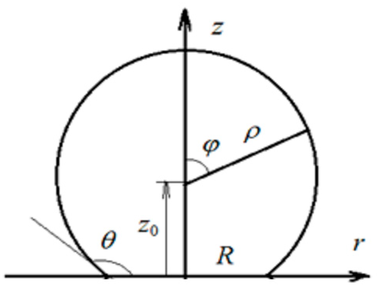
Figure 2. Comparison of exact (4) and approximate (10) formulas for calculating the evaporation flux density of sessile drop. (a) contact angle

\frac{π}{180}

: at the top - graphs of functions (4) and (10), bottom - relative error of the approximate formula in percent; (b) the same for contact angle

\frac{π}{6}

Figure 2. Comparison of exact (4) and approximate (10) formulas for calculating the evaporation flux density of sessile drop. (a) contact angle

\frac{π}{180}

: at the top - graphs of functions (4) and (10), bottom - relative error of the approximate formula in percent; (b) the same for contact angle

\frac{π}{6}

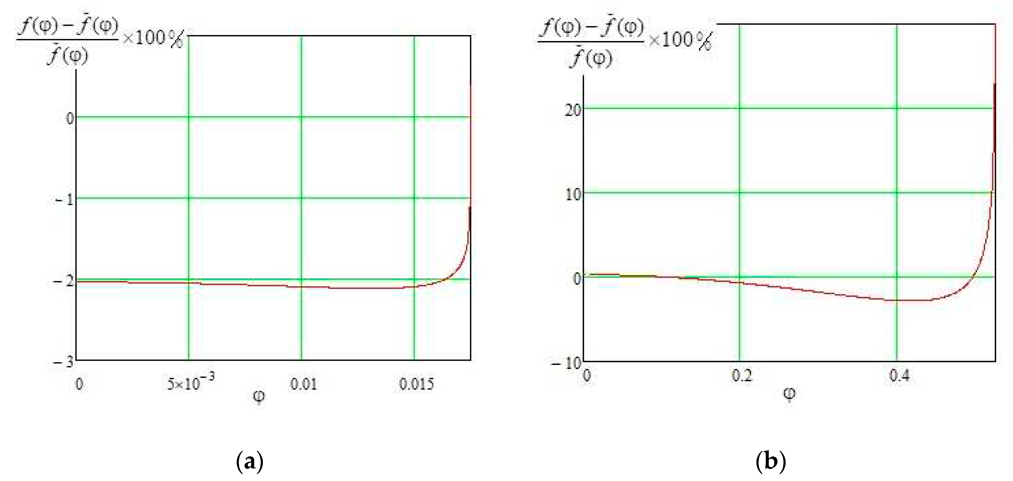
Figure 3. Graphs of the functions represented by formulas (28) and (29).

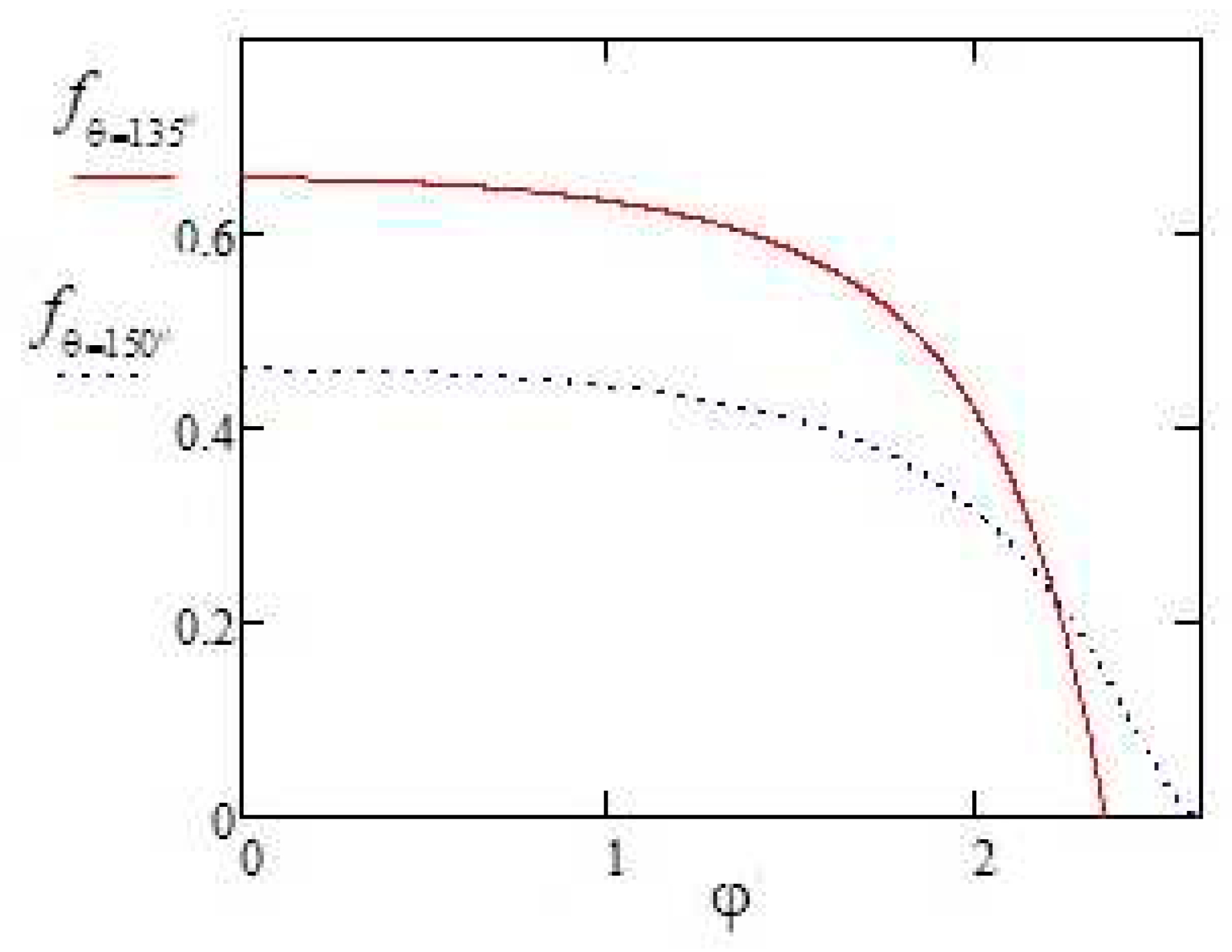
Figure 4. (a) approximate

\overset{⌣}{g} (θ)

and exact

g (θ)

solutions describing evaporation rate of sessile droplet depending on contact angle; (b) relative error of the approximate formula (30) in percent over the entire range of contact angles

[0, ​ ​ ​ π]

Figure 4. (a) approximate

\overset{⌣}{g} (θ)

and exact

g (θ)

solutions describing evaporation rate of sessile droplet depending on contact angle; (b) relative error of the approximate formula (30) in percent over the entire range of contact angles

[0, ​ ​ ​ π]

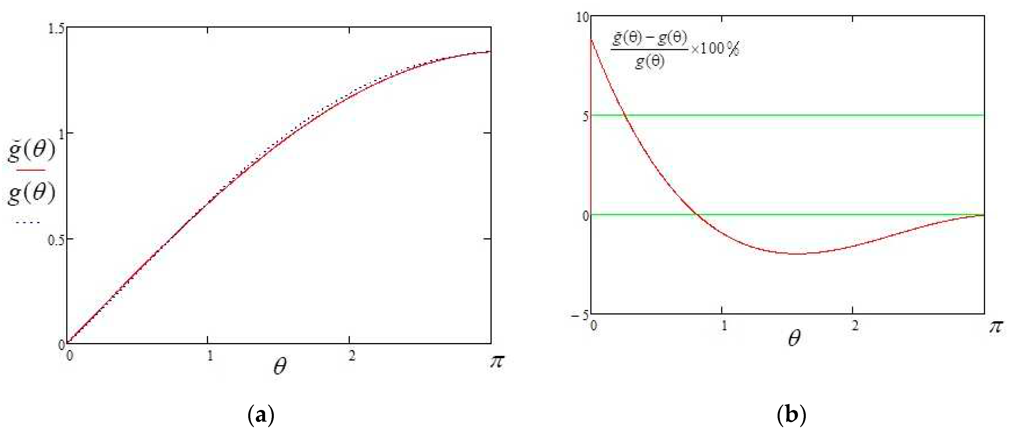
Figure 5. Evaporation time of a drop with an initial contact angle of 110 deg in different evaporation modes as a function of

V^{\frac{2}{3}}

. The CCR mode was calculated by equation (40a), and CCA mode was calculated by equation (41).

Figure 5. Evaporation time of a drop with an initial contact angle of 110 deg in different evaporation modes as a function of

V^{\frac{2}{3}}

. The CCR mode was calculated by equation (40a), and CCA mode was calculated by equation (41).

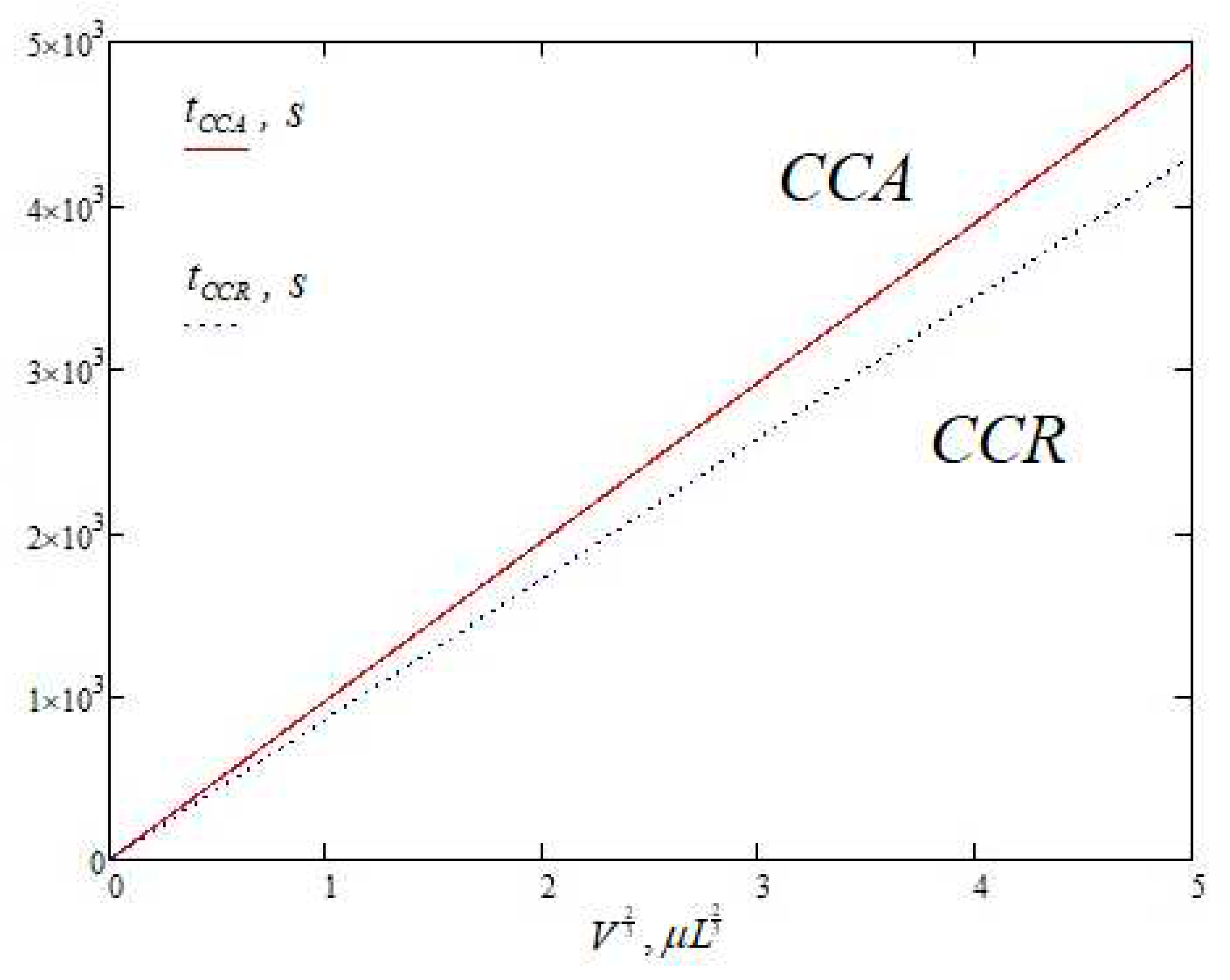
Figure 6. Comparison of exact (4) and approximate (50) expressions for calculating the evaporation flux density of sessile drop: (a) graphs of functions (4) and (50) for the acute contact angles

\frac{π}{180}

(top) and

\frac{π}{6}

(bottom); (b) the same for the obtuse contact angles

\frac{2 π}{3}

(top) and

\frac{170 π}{180}

(bottom).

\frac{π}{180}

(top) and

\frac{π}{6}

(bottom); (b) the same for the obtuse contact angles

\frac{2 π}{3}

(top) and

\frac{170 π}{180}

(bottom).

(a)

(b)

Table 1. First three solutions for evaporation flux density J (contact angles of 90 deg, 135 deg and 150 deg.

j	$θ$		J
1	$π (1 - \frac{1}{2}) = \frac{π}{2} = 90 \deg$	$J = \frac{(n_{s} - n_{\infty}) D}{R}$
2	$π (1 - \frac{1}{4}) = \frac{3 π}{4} = 135 \deg$	$J = \frac{(n_{s} - n_{\infty}) D}{R} (\frac{1}{\sqrt{2}} - \frac{0.25}{{(\frac{3}{2} + \sqrt{2} \cos φ)}^{\frac{3}{2}}})$
3	$π (1 - \frac{1}{6}) = \frac{5 π}{6} = 150 \deg$	$J = \frac{(n_{s} - n_{\infty}) D}{2 R} (1 + {(7 + 4 \sqrt{3} \cos φ)}^{- \frac{3}{2}} - 2 {(4 + 2 \sqrt{3} \cos φ)}^{- \frac{3}{2}})$

Disclaimer/Publisher’s Note: The statements, opinions and data contained in all publications are solely those of the individual author(s) and contributor(s) and not of MDPI and/or the editor(s). MDPI and/or the editor(s) disclaim responsibility for any injury to people or property resulting from any ideas, methods, instructions or products referred to in the content.

© 2023 by the authors. Licensee MDPI, Basel, Switzerland. This article is an open access article distributed under the terms and conditions of the Creative Commons Attribution (CC BY) license (http://creativecommons.org/licenses/by/4.0/).

Copyright: This open access article is published under a Creative Commons CC BY 4.0 license, which permit the free download, distribution, and reuse, provided that the author and preprint are cited in any reuse.

Downloads

112

Views

Comments

Subscription

Notify me about updates to this article or when a peer-reviewed version is published.

MDPI Initiatives

Important Links

Choose an area of interest and we will send you notifications of new preprints at your preferred frequency.

Disclaimer

Evaporation of Small Sessile Drop Deposited on Horizontal Solid Surface: New Exact Solutions and Approximations

Abstract

Keywords:

Subject:

1. Introduction

2. New exact solutions for some values of contact angles

3. New approximate solutions

3.1. Total evaporation rate

3.1. Evaporation flux density for acute and obtuse contact angles

4. Discussion

Author Contributions

Funding

Institutional Review Board Statement

Informed Consent Statement

Data Availability Statement

Conflicts of Interest

References

MDPI Initiatives

Important Links

Subscribe