1. Introduction
The task of visual object tracking is to maintain focus on a specific object in a continuous video, which is one of the fundamental tasks of computer vision and can be applied in autonomous driving, video surveillance, and UAV navigation. Correlation-based trackers calculate the relevance between the template and the search region to determine the position of the target [
1,
2], which can run at ultra-real-time speeds, but its performance is relatively poor due to the limitation of the simple model itself. In recent years, Siamese-based trackers have become a mainstream research direction [
3,
4,
5,
6,
7] , which utilizes weight-sharing neural networks to extract features of the template and the search region, and predicts the target location by calculating the similarity between them. Incorporating robust deep features has led to significant performance gains for Siamese trackers. However, this also requires expensive computational and storage capacity. Also, most trackers that use deep features are characterized by something other than real-time performance.
Transformer [
8] has demonstrated excellent performance in different vision domains, including video understanding [
9], object detection [
10,
11], image classification [
12,
13]. Recently, researchers have adapted the Transformer to object tracking and achieved state-of-the-art performance. However, the large number of matrix multiplication computations required by the attention mechanism therein has dramatically slowed down the inference while improving the performance, for example, the recent SeqTrack [
14] and MixFormer [
15], which, although they achieved 72.5% and 70.0% success rates on the LaSOT dataset, respectively, utilized 535.85G and 113.02G model Flops and 308.98M and 195.40M parameters for the best results. At the same time, their speeds were only 5.81 and 8.02 FPS [
16]. Despite the increasing demand for real-time trackers for human-computer interaction and UAV navigation, efficient tracking architectures (especially Transformer-based ones) have received less attention.
E.T.Track [
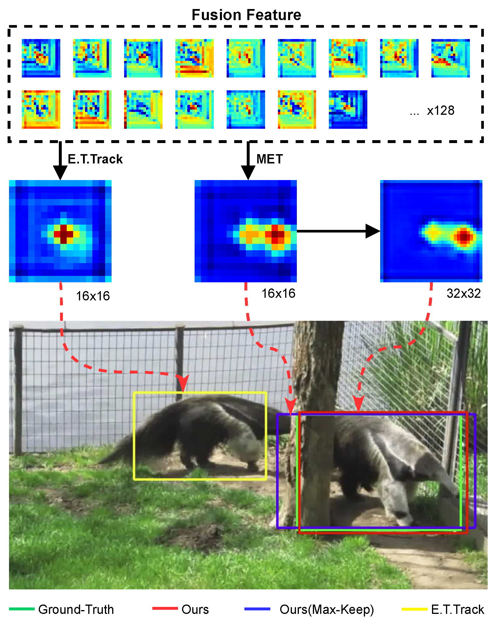
17] was the first to implement real-time tracking using Transformer. It utilizes the exemplar attention to simplify the tracking model with robustness and real-time performance. Expressly, exemplar attention assumes that when tracking a single object, a global query value is sufficient to describe the information available for tracking, capturing more explicit details on the target object relative to the correlation between the various local features of the standard attentional modeling. At the same time, the dataset samples are abstracted into a small set of learnable parameters that constitute the key values used to compute attention. However, E.T.Track views each response in the feature equally when changing the spatial dimensions of the feature map using 2D Adaptive Average Pooling. This inevitably introduces a large amount of background information in the compressed representation of the features, as shown in
Figure 1, which affects target localization. Further, E.T.Track’s feature channel adjustment strategy and compression of feature spatial dimensions to simplify the computation results in loss of information or introduction of redundant data, which can interfere with the accuracy of the bounding box.
Therefore, to solve these problems, as shown in
Figure 1, based on the exemplar Transformer, we utilize scaling-invariant max-filtering to suppress the interference before projecting the compressed representation into the query space, forming the enhancement Transformer, which screens the points from the feature to filter the suspected targets to be copied and maintained, KeepTrack [
18] supports this kind of idea, followed by 2D Adaptive Average Pooling. In addition, to reconstruct the lost information, we borrow from EMSAv2 [
19] and utilize Pixel-Shuffle [
20] to perform an up-sampling operation on the input feature of the enhancement Transformer, i.e., quadruple its spatial area to obtain fine-grained descriptions of the targets. Scaling-invariant max-filtering and Pixel-Shuffle are both very lightweight and have negligible impact on the tracker speed.
We demonstrate the proposed method on 5 benchmarks: LaSOT [
21], OTB100 [
22], UAV123 [
23], NFS [
24], and GOT-10K [
25]. Our proposed tracker runs at 46.8 FPS on the CPU, achieving a new state-of-the-art level, effectively bridging the Transformer with real-time object tracking, and providing a theoretical basis for deployment on resource-constrained devices. The main contributions of this work are as follows:
We design scaling-invariant max-filtering to suppress the background expression in the feature and filter the suspected targets to be enhanced and maintained, improving target localization accuracy;
We utilize Pixel-Shuffle to reconstruct the lost information, increasing the fine-grained level of the feature map and making the bounding box more compact;
We designed a large number of experiments and verified the effectiveness of our proposed method.
We organize this work as follows:
Section 2 reviews the work closely related to our approach.
Section 3 describes the architecture of AnteaTrack.
Section 4 presents the implementation of AnteaTrack and analyzes the experimental results.
Section 5 examines the strengths and weaknesses of AnteaTrack.
Section 6 summarizes this work.
2. Related Work
This section first introduces Siamese tracking, which forms the backbone of our proposed tracker, then the efficient tracking architecture, and finally, the Transformer-based tracker.
2.1. Siamese-Based Tracker
Siamese trackers utilize a weight-sharing backbone network to process template and search frames, and then obtain the target’s location by calculating the similarity between the template and the search features. SiamFC [
3] is a pioneering work on Siamese trackers with a simple structure but performance comparable to the state-of-the-art correlation-based trackers of the time. The SiamRPN [
4] utilizes a regional proposal network(RPN) [
26] to model the tracking problem as a local one-shot detection task and dispenses with online fine-tuning and multi-scale testing. Zhang [
6] found that the anchor-based Siamese tracker is trained only on positive anchor frames. This mechanism relies heavily on the distribution probabilities of the anchor frames at the time of initialization, thus making it difficult to find the target’s location when the overlap between the anchor frames and Ground-Truth is small. Therefore, it utilizes the anchor-free approach to directly predict the location and scale of the target object while utilizing deformable convolution to perceive the target object adaptively. The Siamese idea has been widely used in visual object tracking, including long-term tracking [
27,
28], fusion tracking [
29,
30], and real-time tracking [
7,
17].
2.2. Efficient Tracker
The fast development of UAV navigation and autonomous driving has expanded the demand for real-time visual object tracking. More extensive models and more parameters do trade-offs for better performance, but at the same time seriously affect the tracker’s speed. Lightweight trackers can solve this problem [
2,
31]. Methods such as KCF [
1] and fDSST [
32] based on correlation filtering can run at ultra-real-time speeds on computationally limited devices. However, limited by the expressive power of handcrafted features, it isn’t easy to satisfy the application requirements in terms of accuracy and robustness. LightTrack [
7] absorbs the idea of a one-shot neural architecture search(NAS), trains in a more extensive search space single hyper-parameterized weight-sharing model, and then determines the final architecture of the tracker by an evolutionary algorithm. E.T.Track [
17], most relevant to this work, designed an efficient Transformer structure and took the same backbone as LightTrack to implement the first Transformer-based real-time tracker. However, it uses Adaptive Average Pooling to directly down-sample the feature maps into vectors with spatial dimensions of
, a process that treats background and foreground equally, which can affect the judgment of the tracker. Therefore, we add scaling-invariant max-filtering before this, which is used to highlight the features of the suspected target while keeping the spatial dimension constant. In addition, E.T.Track performs channel adjustment on features from the backbone, which can cause information loss, so we used Pixel-Shuffle to refine the feature representation, thus compensating for it.
2.3. Transformer-Based Tracker
Recently, Yan [
33] introduced Transformer into target tracking and achieved good performance. Transformer-based tracking can be divided into two categories [
16]. One is CNN-Transformer-based trackers [
33,
34,
35,
36]. These trackers usually use a backbone based on the structure of the convolutional neural network to extract the template and the search region features, respectively, and then use Transformer to fuse the two region’s features, but due to the presence of CNN, Transformer cannot model the global information of the original image, so another class of paradigms uses the structure based on fully-Transformer. Specifically, this class of trackers can be categorized into Two-stream Two-stage type, which has a similar framework to the CNN-Transformer based trackers, but it uses the Transformer to produce the backbone, as in [
37,
38,
39]. While the latter considers feature extraction and fusion as a single stage [
15,
40,
41,
42]. According to the above categorization, AnteaTrack belongs to the CNN-Transformer-based architecture. However, our tracker pays more attention to inter-sample rather than intra-sample correlation when dealing with features from the backbone [
17].
3. Methods
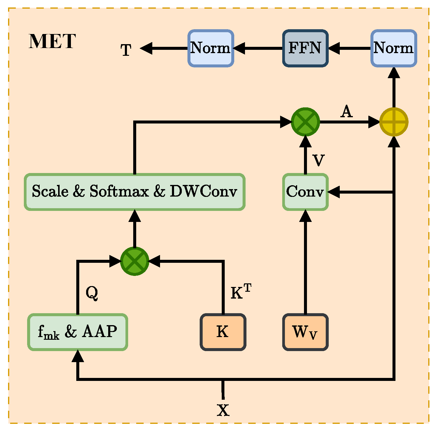
This section first introduces our proposed enhancement Transformer, which consists of two modules. Firstly, we use scaling-invariant max-filtering to filter out the suspected targets, as shown in
Figure 2. Then, based on the former, the features are spatially scaled using Pixel-Shuffle. Then the standard Transformer is introduced, and finally, the tracker framework proposed in this work is presented.
3.1. Standard Transformer
The proposal of Transformer [
8] has led to the widespread use of the attention mechanism in various domains, which is a sequential model that can be represented as
where
represents N feature vectors of dimension D, and the
means the FeedForward Network.
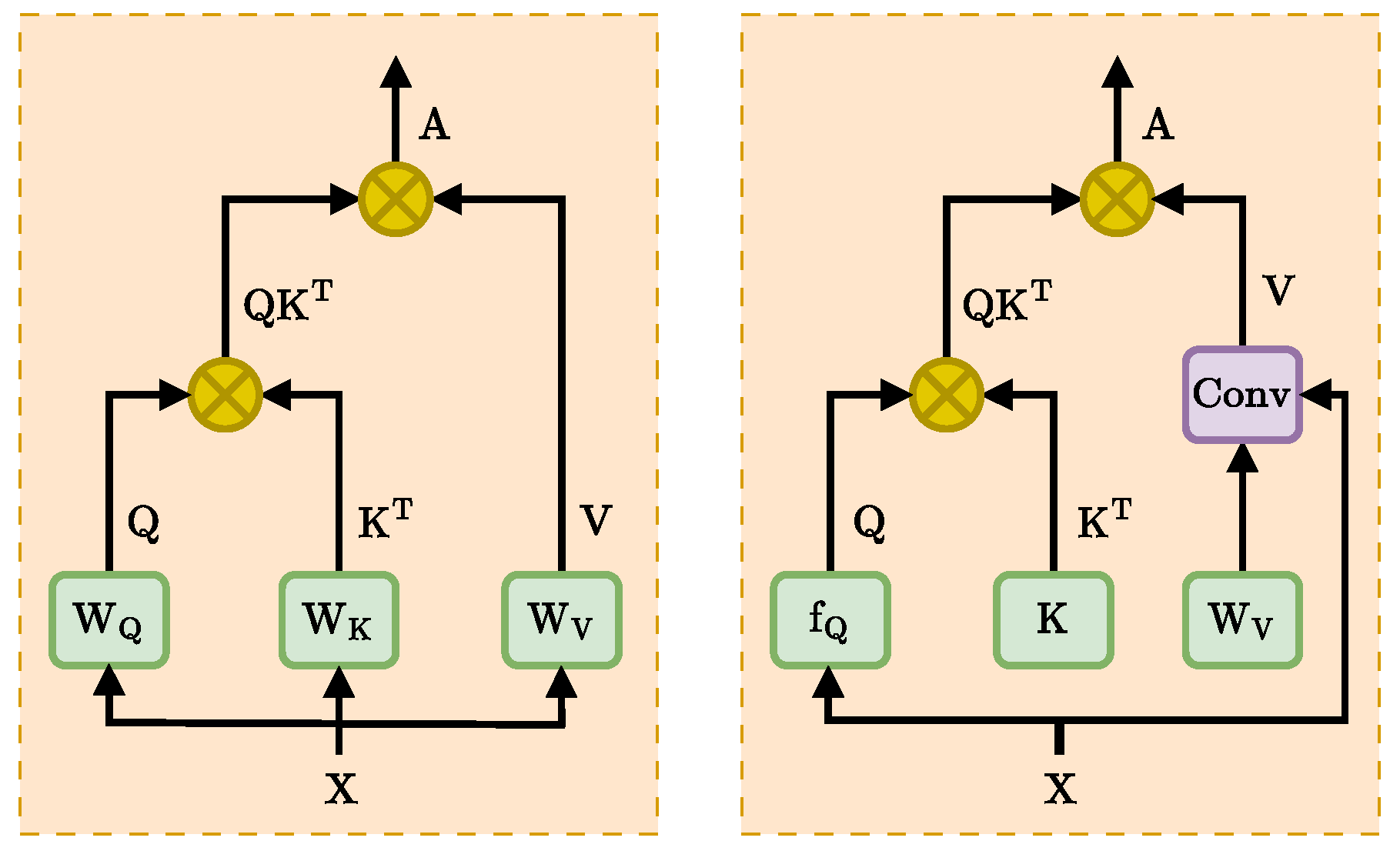
represents the self-attention mechanism, as shown in
Figure 3. The input sequences are abstracted as "query(Q),” "key(K)," and "value(V)" by multiplying with the learnable parameter matrix. Then, the Q and K are computed by dot product to get the similarity scores among all features, and finally, the output of the attention mechanism is calculated by multiplying with V, which is denoted as
, , and denote the learnable parameter matrix, and indicates the normalization constant, which limits the range of similarity. In this work, .
3.2. Scale-Invariant Max-Filtering Enhancement Transformer
There are local correlations between neighboring pixels of a 2D image, and they usually correspond to the same object. Therefore, the visual Transformer utilizes patch embedding to segment the image and map it to a lower dimensional space, which is then processed with the attention mechanism [
12]. In contrast, the exemplar Transformer pays more attention to the correlation between samples, as shown in
Figure 3. In its core component exemplar attention, the feature
is down-sampled using a 2D Adaptive Average Pooling operation with output spatial dimension
, which
denotes the spatial dimension of the feature,
. Then, it is projected to the query space to form Q using the parameter matrix, which can be expressed as
where
indicates that the input
X is down-sampled, Adaptive Average Pooling directly averages all feature components and aggregates them into a
feature vector. This introduces a large amount of background information that interferes with the accurate representation of the target.
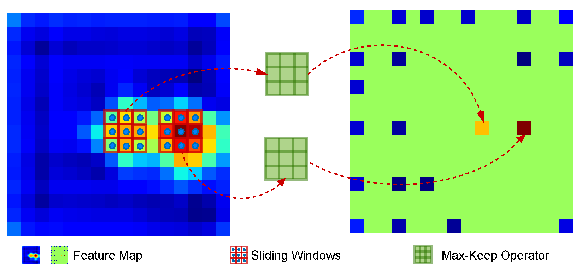
Therefore, as shown in
Figure 4, we design a scaling-invariant max-filtering operator for filtering out suspected targets before average pooling. Specifically, we use a sliding window of size
, stride
to sample the 2D feature maps and filter out the largest response used to replace the centroid, i.e., the suspected target, by max-pooling within the sampled region. As shown in
Figure 1, the center of the second row represents the classified features after MET processing, which effectively suppresses the background and enhances the expression of the suspected target. In addition, it ensures the structural integrity of the image. Then Q can be defined as
we refer to
as the max-keep function, which does not change the features’ spatial scale and introduces learnable parameters, thus consuming negligible computation and storage.
Keys and values are derived from linear transformations of serialized inputs, therefore, contain fewer local correlations and contextual relationships relative to convolution [
17]. However, in exemplar attention, inter-sample relationships are more critical than intra-sample relationships, so keys are treated as input-independent learnable parameters
, which
represents the number of exemplars. It encapsulates the dataset information to form instance-level exemplar representations, which can be flexibly adapted to the attention layer after interacting with the query. For values, the input is combined with the parameter matrix
using convolution rather than projection, with
Z representing an arbitrary spatial dimension. Thus, the value V can be defined as
where ⊛ denotes the convolution operation, the spatial bias built into the convolution provides a suitable generalization of the local information and a good inheritance of the output features from the backbone.
Finally, our scaling-invariant max-filtering enhancement attention can be expressed as
3.3. Fine-Grained Feature Representation with Pixel-Shuffle
Both the channel adjustment and the compressed input representation introduce redundancy or cause loss of information. As shown in
Figure 1, the MET output features lead to accurate target localization, but their bounding boxes need to be more precise. Therefore, we use Pixel-Shuffle to up-sample the feature in the spatial dimension before feeding it into the enhancement Transformer, refining the feature representation of the target counterpart to obtain a more compact bounding box. Thus, Equation (
6) can be expressed as
where
denotes the operation of spatial dimension increase using Pixel-Shuffle.
Pixel-Shuffle achieves the effect of increasing the spatial dimensionality by rearranging the features sampled on the channel, and, with a small number of learnable parameters, it can remove redundant data to a certain extent while improving the accuracy of the feature description. It consists of a single layer of convolution, therefore, has little effect on the efficiency of the tracker.
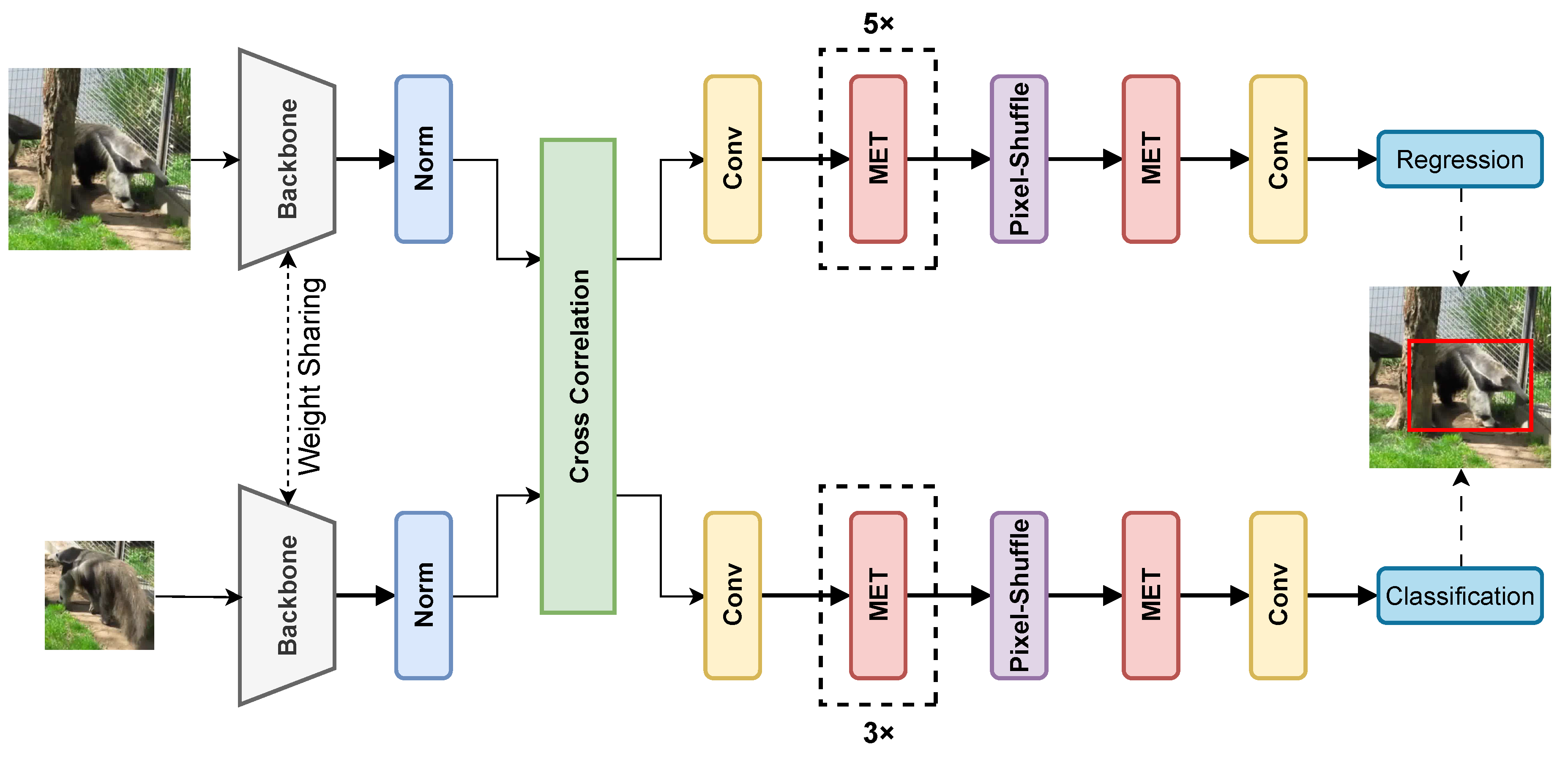
3.4. AnteaTrack Architecture
Figure 5 shows the flowchart of our proposed tracker. Based on the Siamese network, we use a weight-sharing lightweight backbone LT-Mobile [
7] to extract the features of the template and the search region. To improve the convergence speed, we process the output features of the backbone using a layer normalization and then fuse them using a pixel-level cross-correlation with channel tuning. Typically, the information requirements for classification and regression are not symmetric, with larger receptive fields capturing broader contextual information and smaller ones localizing features favorably and providing accurate location predictions. Therefore, we articulate a convolutional layer of size
and
at the end of the classification and regression branches and adjust the feature channels again.
The classification branch categorizes the search region into foreground and background, and the regression branch predicts the distance to the four sides of the bounding box. Therefore, we superimpose three and five METs in the two branches, respectively, then increase the spatial dimensionality of the features using Pixel-Shuffle, and finally end the branch using one MET. It is worth noting that when the spatial resolution of the features is increased, there is also a concomitant increase in the fine-graininess of the target. Therefore, in the MET module before and after Pixel-Shuffle, we use pooling kernels of different sizes, specifically, taking
when the spatial scale of the features is small and
is large. Finally, a single-layer convolution synthesizes the classification and regression features to obtain the target’s location and the bounding box prediction information. Based on the idea of an anchor-free fashion, in the training phase, we use the IoU loss [
43] to optimize the distance to the four sides of the bounding box. For the location prediction of the target, the binary cross entropy(BCE) loss is utilized for limiting.
4. Experiments and Analysis of Results
In this section, we first present the training and testing details of the tracker. Then, we compare the performance of our method with state-of-the-art methods on 5 datasets. Finally, we show the ablation study of the module proposed in this work.
4.1. Experimental Requirements and Implementation Details
We use two NVIDIA GeForce RTX 3090 GPUs for joint training. Specifically, the initialized weights of the backbone on ImageNet [
44] are loaded and trained for a total of 50 epochs, the parameters of the backbone are frozen, and the gradient update is removed for the first 10 epochs. For the first 5 epochs, the learning rate is adjusted from 0.02 to 0.1 using a step learning rate scheduler to "warm up" the model. The logarithmic learning rate scheduler is used for the remaining epochs to reduce the learning rate to 0.0002. The whole model is optimized using stochastic gradient descent(SGD) [
45], with a momentum of 0.9 and weight decay of 0.0001. In each epoch, we randomly sample 64k image pairs from LaSOT [
21], GOT10K [
25], and COCO [
46] at sampling intervals of 100, 30, and 1 frames [
17], respectively, using 32 image pairs per iteration for a total of 2000 iterations. Each image pair consists of a search frame and a template frame, which are pre-processed with random gray-scaling as well as jitter brightness, and, based on the Ground-Truth and the search scale factor(4 for the search and 2 for the template), cropped and scaled to
and
pixel sizes to form the search and template regions, respectively.
In the testing phase, we used an Intel(R) Core(TM) i5-10400F CPU @ 2.90GHz and preprocessed the images normalized in the channel dimension.
4.2. Evaluation Datasets and Analysis of Results
In this subsection, we compare non-real-time trackers (SiamRPN++ [
5], TransT [
34], TrDiMP [
36], OSTrack [
41], MATTrack [
47], MixFormer [
15], STARK [
33], TrSiam [
36], DiMP [
48], PrDiMP [
49]) and real-time trackers (KCF [
1], ECO [
2], LT-Mobile [
7], E.T.Track [
17]) to our tracking methods and report results on 5 datasets including GOT-10K [
25], LaSOT [
21], UAV123 [
23], OTB100 [
22], and NFS [
24].
4.2.1. GOT-10K Dataset and Analysis of Evaluation Results
GOT-10K [
25] is a large-scale dataset containing 10k high-resolution video sequences and more than 1.5 million bounding boxes, consisting of 9335 training, 180 validation, and 180 testing sequences covering multiple categories and motion patterns of field objects. In addition, the developers of GOT-10K built an online evaluation server to present the tracker as a leaderboard. We ran AnteaTrack on the testing sequences and obtained the official evaluation results in
Table 1.
GOT-10K uses the average overlap rate
and the success rate
with thresholds of 0.5 and 0.75, respectively, as evaluation metrics. As shown in Table 1, AnteaTrack obtains a performance improvement of 2.7% on
and 4.9% and 4.0% on
and
, respectively, relative to the baseline E.T.Track [
17]. GOT-10K contains a large number of field scenes with similar targets. MET suppresses the background while suppressing the similar targets. After obtaining relatively accurate localization, the fine-grained features brought by Pixel-Shuffle provide more compact bounding boxes.
4.2.2. OTB100 Dataset and Analysis of Evaluation Results
The OTB100 [
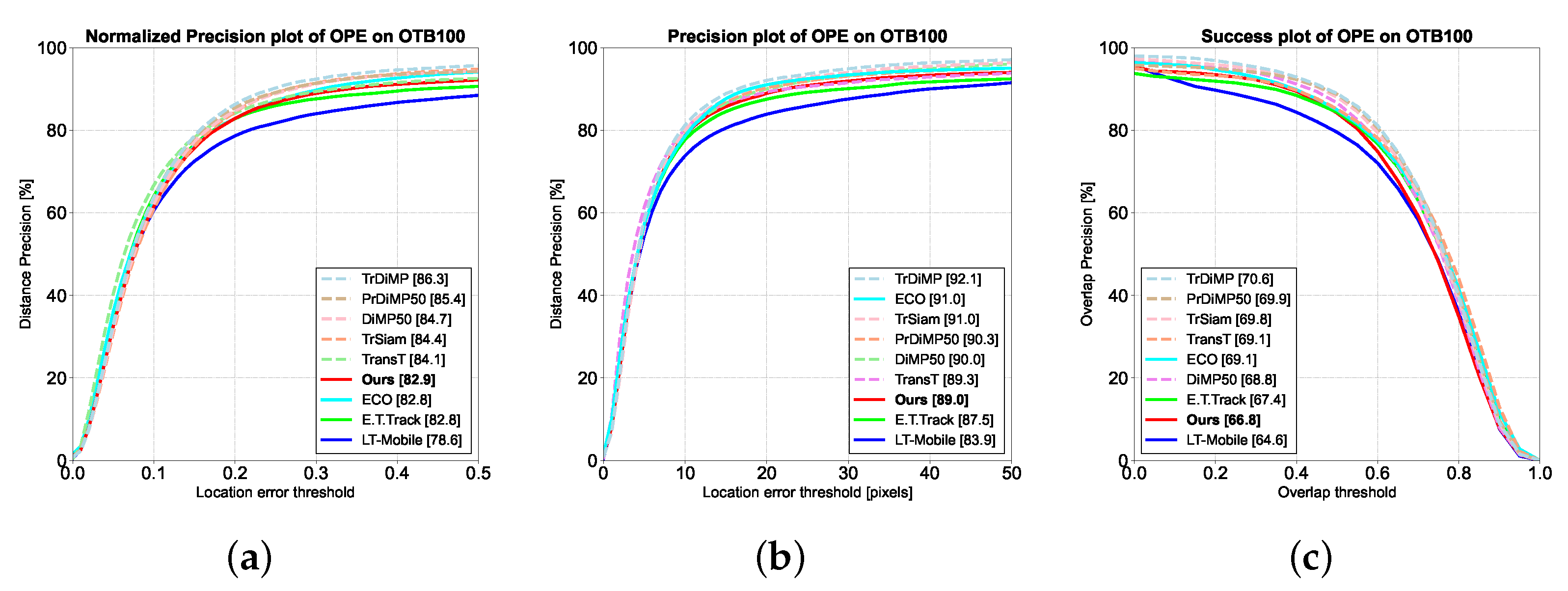
22] dataset contains 100 video sequences with 25 grayscale sequences containing 11 challenge attributes such as occlusion, fast motion, and background clutter. OTB100 defines the paradigm of using only the first frame of a sequence to initialize the tracker and complete the remaining picture inference as a one-pass evaluation(OPE). We evaluated AnteaTrack on OTB100 and reported the results in
Figure 6.
OTB100 uses the precision and success rates in OPE as metrics, and to balance the impact of image resolution and bounding box size on the precision, we also evaluated the normalized precision proposed in [
50]. As shown in
Figure 6, we outperform it and other real-time trackers in terms of normalized precision compared to the baseline, gaining a 1.5% performance improvement in precision to 89.0% and performing comparably in terms of success rate. MET can retain suspected targets, but due to the low resolution of the images contained in the OTB100, this can result in the output features of the backbone not being robust enough to affect the judgment of MET. In addition, the backbone of the ECO [
2] algorithm provides more shallow depth features. Therefore, it outperforms some non-real-time tracking algorithms regarding success and precision.
4.2.3. UAV123 Dataset and Analysis of Evaluation Results
The UAV123 [
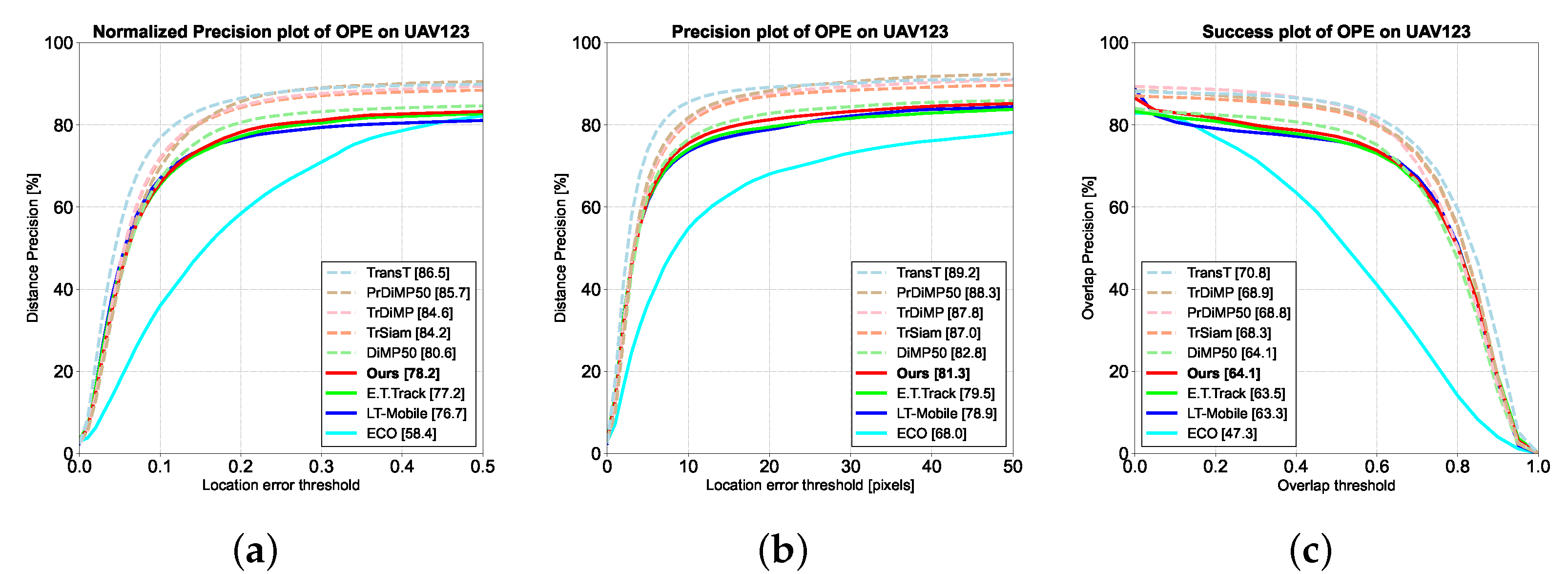
23] dataset contains 123 high-definition videos captured from low-altitude UAV viewpoints, totaling more than 110k frames with 12 challenge attributes. Unlike the above datasets, its viewpoints, altitudes, and motion patterns have been changed. We ran AnteaTrack on UAV123 and reported the tracking results in
Figure 7.
The metrics for UAV123 are the same as for OTB100 [
22]. As shown in
Figure 7, we achieved 76.9% and 81.7% in normalized precision and precision, obtaining 1.2% and 1.6% performance gains relative to E.T.Track [
17]. Regarding success rate, 62.3% was achieved, only 1.9% different from the non-real-time tracker DiMP50 [
48]. MET suppresses some background representations, while Pixel-Shuffle provides more detailed characterization, effectively tracking UAV123 with more small targets. In addition, we compare AnteaTrack with other trackers based on the challenge properties of UAV123 in sub
Section 4.3.
4.2.4. LaSOT Dataset and Analysis of Evaluation Results
The LaSOT [
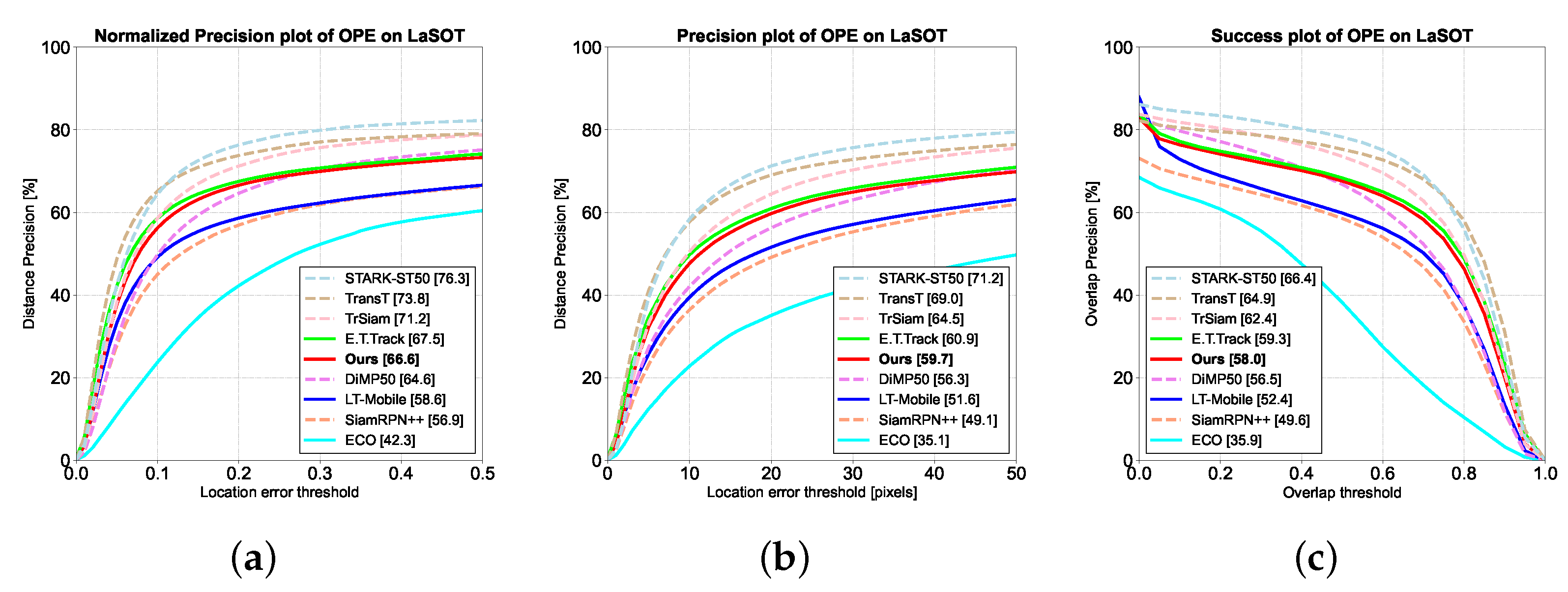
21] dataset consists of 1400 video sequences, of which 280 were used for testing. With more than 3.5M images from 70 categories, individual sequences are at least 1000 frames long, and targets may disappear briefly. We evaluated AnteaTrack on LaSOT’s test sequences and reported the results in
Figure 8.
LaSOT was evaluated on the same metrics as OTB100 [
22]. As shown in
Figure 8, AnteaTrack achieves 66.6% and 59.2% in normalized precision and precision, respectively, gaining 2% and 2.9% performance improvement over the non-real-time tracker DiMP50 [
48] and 1.5% performance improvement in success rate. However, E.T.Track [
17] slightly outperforms AnteaTrack on LaSOT. When the target is out-of-view, MET considers the most similar counterpart in the search area as the target. It suppresses the rest of the background, while it is more challenging to achieve re-finding when the target reappears due to the limitation of the search area. A more detailed analysis is provided in
Section 5.
4.2.5. NFS Dataset and Analysis of Evaluation Results
The NFS [
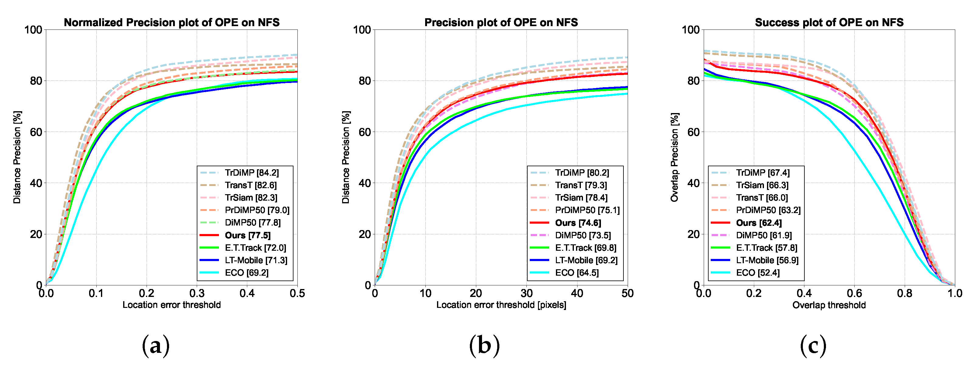
24] dataset explores the possibility of object tracking at higher video frame rates. It consists of 100 video sequences with a total number of video frames of about 380k and contains a subset of videos with two frame rates. We evaluated AnteaTrack on a subgroup of 30FPS and presented the results in
Figure 9.
The metrics for NFS are the same as OTB100 [
22]. As shown in
Figure 9, AnteaTrack improves the normalized precision by 5.5% compared to E.T.Track [22], with a precision of 74.6%, an improvement of 4.8%. The success rate is improved by 4.6%, surpassing DiMP50 [
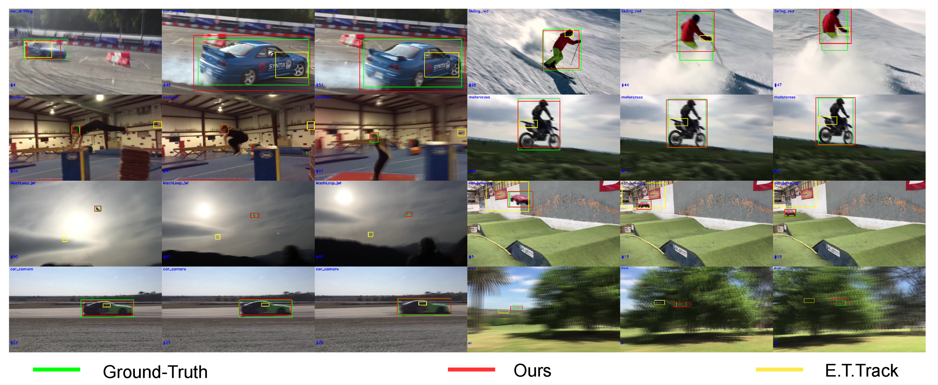
48]. NFS contains motion-blurred frames whose target counterparts must be sufficiently well-defined, resulting in missing detail information, while residual shadows introduce redundancy. As shown in
Figure 10, E.T.Track suffers from situations such as tracking drift or large deviations in the bounding box, but motion blur has little effect on AnteaTrack. This is because MET first filters out the suspected targets from a large amount of background information(equivalent to deblurring), then selects from among them. In addition, Pixel-Shuffle also removes redundant data due to residual shadows, leading to relatively accurate target localization and bounding boxes.
4.3. Attribute-Based Performance on UAV123
The UAV123 [
23] dataset has 12 challenge attributes: Aspect Ratio Change (ARC), Background Clutter (BC), Camera Motion (CM), Fast Motion (FM), Full Occlusion (FOC), Illumination Variation (IV), Low Resolution (LR), Out-of-View (OV), Partial Occlusion (POC), Similar Object (SOB), Scale Variation (SV) and Viewpoint Change (VC). We evaluated AnteaTrack based on attributes, and the results are shown in
Table 4. Compared to the baseline, AnteaTrack outperforms it in normalized precision on all attributes, with a slightly lower precision for LR and a somewhat weaker success for IV. Both low-resolution and illumination variations blur the boundary between the target and the background. MET’s property of suppressing the ground may discriminate suspects as targets, leading to tracking drift.
4.3.1. Pixel-Shuffle
We report the gains made by Pixel-Shuffle in
Table 2 and explore the performance of scaling-invariant max-filtering for combining different branches.
Table 3 reports the performance impact of similar methods, "Nearest " and "Bilinear Interpolation." In addition, Pixel-Shuffle changes the spatial scale of the features, so it is impossible to explore its implications in a separate branch.
As shown in
Table 2, E.T.Track [
17] provides relatively inaccurate target localization that cannot be corrected when only Pixel-Shuffle is used, resulting in a relatively small performance gain of only 1.8% on the GOT-10K [
25] and virtually no gain on UAV123 [
23]. The target size is small in UAV123, so fine-grained features have little effect on the accuracy of the bounding box. However, the impact is more significant in the presence of scaling-invariant max-filtering in the classification, gaining a 3% improvement on GOT-10K, and the most gains are made when we use scaling-invariant max-filtering and Pixel-Shuffle jointly.
Not all spatial resolution improvements result in enhancements. As shown in
Table 3, the "Nearest" and "Bilinear Interpolation" methods decrease by 21.5% and 22.6, respectively. They are simple methods that determine the value of the current pixel based on the value of the nearest pixel; however, deep features contain more semantic information, and these methods treat them in an unlearnable way, which destroys the original information structure and causes performance degradation.
Table 4.
Performance comparison of AnteaTrack on the 12 challenge attributes of UAV123 [
23]. The gray portion of the table is for non-real-time trackers, with the best scores in
blue, while the best results for real-time tracking in
red. (a), (b) and (c) represent the normalized precision, precision and success respectively, "↑" indicates an improvement relative to baseline and vice versa.
| (a) Normalized precision |
|---|
| |
non-real-time |
real-time |
| |
TrDiMP
[36]
|
TrSiam
[36]
|
DiMP50
[48]
|
PrDiMP50
[49]
|
TransT
[34]
|
ECO
[2]
|
LT-Mobile
[7]
|
E.T.Track
[17]
|
AnteaTrack
(Ours)
|
| ARC |
0.812 |
0.807 |
0.775 |
0.819 |
0.816 |
0.570 |
0.732 |
0.724 |
0.744↑ |
| BC |
0.567 |
0.644 |
0.607 |
0.688 |
0.567 |
0.534 |
0.543 |
0.537 |
0.547↑ |
| CM |
0.821 |
0.849 |
0.827 |
0.862 |
0.859 |
0.650 |
0.788 |
0.768 |
0.788↑ |
| FM |
0.783 |
0.770 |
0.774 |
0.800 |
0.824 |
0.577 |
0.758 |
0.749 |
0.758↑ |
| FOC |
0.614 |
0.659 |
0.599 |
0.677 |
0.625 |
0.484 |
0.549 |
0.498 |
0.571↑ |
| IV |
0.762 |
0.804 |
0.795 |
0.779 |
0.781 |
0.599 |
0.711 |
0.712 |
0.697 ↓ |
| LR |
0.669 |
0.630 |
0.654 |
0.694 |
0.708 |
0.531 |
0.600 |
0.592 |
0.600↑ |
| OV |
0.821 |
0.825 |
0.781 |
0.788 |
0.849 |
0.592 |
0.762 |
0.717 |
0.762↑ |
| POC |
0.755 |
0.761 |
0.743 |
0.785 |
0.784 |
0.591 |
0.661 |
0.669 |
0.693↑ |
| SOB |
0.791 |
0.782 |
0.791 |
0.802 |
0.804 |
0.639 |
0.666 |
0.658 |
0.680↑ |
| SV |
0.795 |
0.792 |
0.782 |
0.814 |
0.824 |
0.633 |
0.746 |
0.732 |
0.747↑ |
| VC |
0.846 |
0.842 |
0.806 |
0.857 |
0.865 |
0.584 |
0.767 |
0.772 |
0.782↑ |
| (b) Precision |
| |
non-real-time |
real-time |
| |
TrDiMP
[36]
|
TrSiam
[36]
|
DiMP50
[48]
|
PrDiMP50
[49]
|
TransT
[34]
|
ECO
[2]
|
LT-Mobile
[7]
|
E.T.Track
[17]
|
AnteaTrack
(Ours)
|
| ARC |
0.851 |
0.842 |
0.808 |
0.851 |
0.840 |
0.654 |
0.760 |
0.762 |
0.787↑ |
| BC |
0.540 |
0.722 |
0.687 |
0.775 |
0.614 |
0.624 |
0.625 |
0.599 |
0.625↑ |
| CM |
0.864 |
0.892 |
0.872 |
0.903 |
0.893 |
0.721 |
0.826 |
0.813 |
0.839↑ |
| FM |
0.842 |
0.823 |
0.832 |
0.858 |
0.860 |
0.652 |
0.800 |
0.793 |
0.803↑ |
| FOC |
0.687 |
0.731 |
0.673 |
0.760 |
0.678 |
0.576 |
0.602 |
0.571 |
0.652↑ |
| IV |
0.809 |
0.850 |
0.847 |
0.838 |
0.816 |
0.710 |
0.757 |
0.757 |
0.751 ↓ |
| LR |
0.767 |
0.720 |
0.747 |
0.790 |
0.772 |
0.683 |
0.673 |
0.677 |
0.674 ↓ |
| OV |
0.835 |
0.835 |
0.790 |
0.797 |
0.857 |
0.590 |
0.767 |
0.743 |
0.795↑ |
| POC |
0.810 |
0.814 |
0.797 |
0.839 |
0.823 |
0.669 |
0.705 |
0.721 |
0.748↑ |
| SOB |
0.848 |
0.833 |
0.800 |
0.848 |
0.850 |
0.747 |
0.716 |
0.725 |
0.763↑ |
| SV |
0.845 |
0.839 |
0.830 |
0.862 |
0.860 |
0.707 |
0.785 |
0.778 |
0.796↑ |
| VC |
0.878 |
0.870 |
0.828 |
0.883 |
0.892 |
0.680 |
0.789 |
0.795 |
0.813↑ |
| (c) Success |
| |
non-real-time |
real-time |
| |
TrDiMP
[36]
|
TrSiam
[36]
|
DiMP50
[48]
|
PrDiMP50
[49]
|
TransT
[34]
|
ECO
[2]
|
LT-Mobile
[7]
|
E.T.Track
[17]
|
AnteaTrack
(Ours)
|
| ARC |
0.643 |
0.639 |
0.601 |
0.645 |
0.648 |
0.445 |
0.585 |
0.581 |
0.594↑ |
| BC |
0.429 |
0.495 |
0.461 |
0.527 |
0.430 |
0.387 |
0.433 |
0.409 |
0.428 ↑ |
| CM |
0.661 |
0.683 |
0.660 |
0.662 |
0.692 |
0.506 |
0.644 |
0.627 |
0.640 ↑ |
| FM |
0.629 |
0.617 |
0.615 |
0.640 |
0.656 |
0.415 |
0.610 |
0.595 |
0.603↑ |
| FOC |
0.435 |
0.474 |
0.422 |
0.491 |
0.444 |
0.308 |
0.386 |
0.353 |
0.416↑ |
| IV |
0.601 |
0.634 |
0.627 |
0.617 |
0.617 |
0.458 |
0.574 |
0.568 |
0.558 ↓ |
| LR |
0.517 |
0.488 |
0.495 |
0.530 |
0.542 |
0.396 |
0.459 |
0.457 |
0.458 ↑ |
| OV |
0.632 |
0.634 |
0.590 |
0.608 |
0.663 |
0.425 |
0.601 |
0.571 |
0.605↑ |
| POC |
0.593 |
0.599 |
0.576 |
0.619 |
0.614 |
0.456 |
0.523 |
0.529 |
0.546↑ |
| SOB |
0.634 |
0.627 |
0.594 |
0.641 |
0.638 |
0.518 |
0.537 |
0.534 |
0.550↑ |
| SV |
0.645 |
0.643 |
0.625 |
0.656 |
0.667 |
0.496 |
0.608 |
0.599 |
0.605 ↑ |
| VC |
0.689 |
0.683 |
0.641 |
0.688 |
0.708 |
0.473 |
0.633 |
0.635 |
0.641↑ |
5. Discussion
Tracking drift often stems from poor handling of several keyframes. AnteaTrack has been improved on GOT-10K [
25], UAV123 [
23], and NFS [
24]. As in
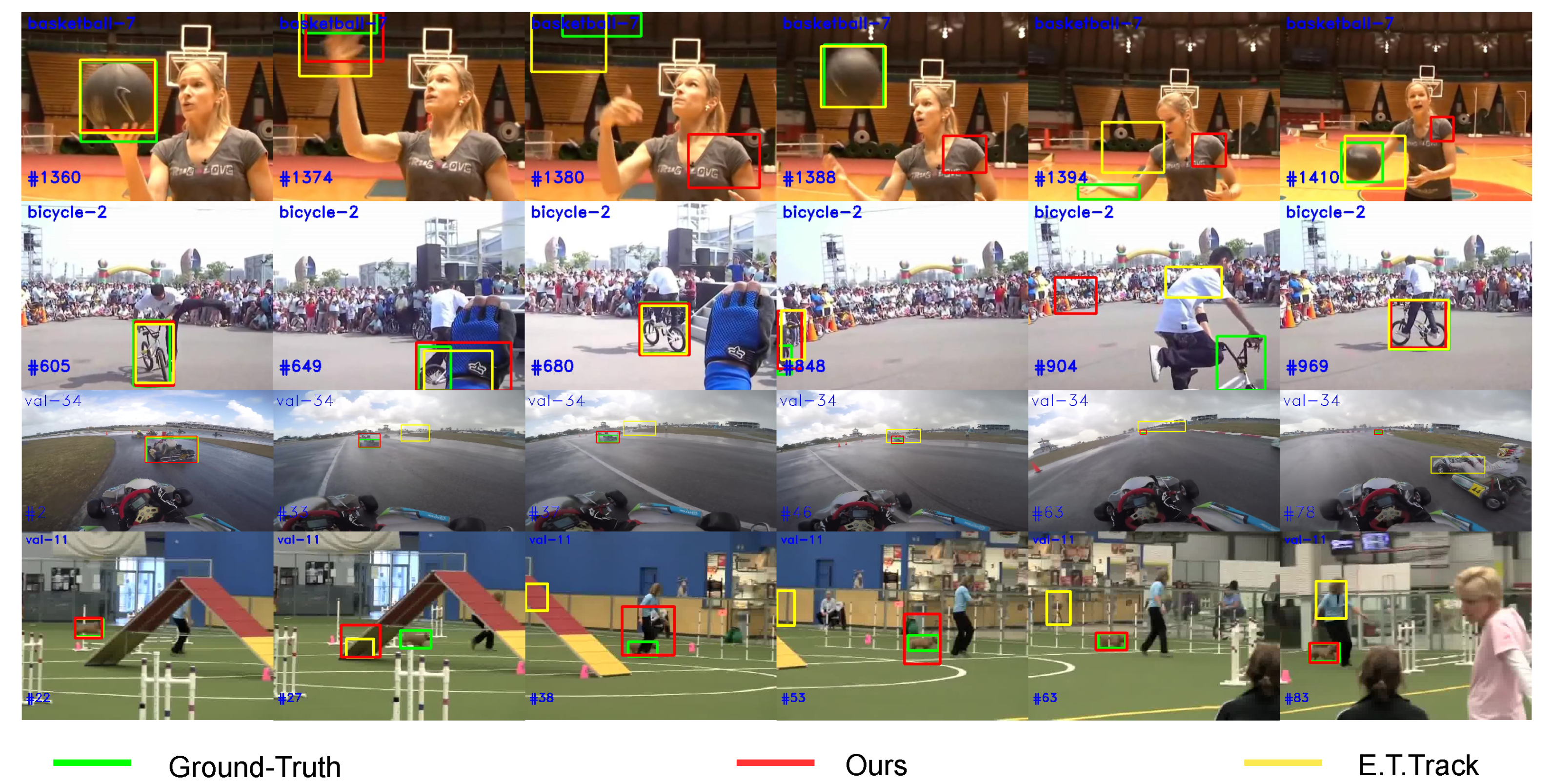
Figure 11, line 1, after the target is briefly out of view, the baseline E.T.Track [
17] can follow it, while AnteaTrack cannot. The target is heavily occluded in the second row, but both trackers successfully retrieve it. For the former, the presence of highly similar objects and the fact that once the scaling-invariant max-filtering operator treats the target as a background, it suppresses it. The predefined search factor limits the region, leading to tracking failure. The latter do not have similarities and can therefore be re-fetched. The last two lines of pictures have even fewer frames, and the target is moving very fast. The E.T.Track drifts considerably, i.e., as shown in (val-34, #46), it briefly returns to the target with a relatively sizeable bounding box but soon drifts again.
The search feature produces more changes relative to the template at higher frame sizes. When the target is out-of-view, the MET prompts AnteaTrack to look for a similarity in the search region and enhance it. At the same time, AnteaTrack’s cosine weighting of the categorized features fails to suppress its expression while being constrained by the search region, failing to retrieve it. However, AnteaTrack can correct for transient drift when the search frame does not co-occur with the out-of-view and similar objects. In addition, MET’s enhancement of suspected targets and suppression of the background allows for more accurate target localization, and Pixel-Shuffle provides refined feature representation to find tighter bounding boxes.
6. Conclusion
In this work, we utilize scaling-invariant max-filtering to suppress the background expression in the search region while enhancing the suspected targets, significantly improving the localization precision. In addition, to obtain a more compact bounding box, we utilize Pixel-Shuffle to enhance the fine-graininess of classification and regression features while compensating for information loss and removing redundancy, and have little impact on speed, being able to run at more than real-time speeds on resource-constrained CPUs. Our tracker handles disturbances such as fast motion, small size, and occlusion well. However, scaling-invariant max-filtering needs a certain degree of learnability, so the robustness of the tracker needs to be improved. Finding a more flexible background suppression method is a direction worth exploring.
Author Contributions
Conceptualization, Xingzhong Xiong; Funding acquisition, Xingzhong Xiong, Fanqin Meng and Jun Liu; Investigation, Zhen Chen; Methodology, Zhen Chen; Project administration, Xingzhong Xiong, Fanqin Meng and Jun Liu; Supervision, Zhen Chen, Xingzhong Xiong, Fanqin Meng, Xianbing Xiao and Jun Liu; Writing – original draft, Zhen Chen; Writing – review & editing, Zhen Chen, Xingzhong Xiong, Xianbing Xiao and Jun Liu.
Funding
This research was funded by the Science and Technology Department of Sichuan Province grant number 2023NSFSC1987, Opening Project of Key Laboratory of Higher Education of Sichuan Province for Enterprise Informationalization and Internet of Things grant number 2022WYJ04 and in part by the Postgraduate Innovation Fund Project of Sichuan University of Science and Engineering grant Y2022120 number and the Artificial Intelligence Key Laboratory of Sichuan Province grant number 2019RZJ04.
Institutional Review Board Statement
Not applicable.
Informed Consent Statement
Not applicable.
Data Availability Statement
Public datasets.
Conflicts of Interest
The authors declare that they have no conflict of interest.
References
- Henriques, J.F.; Caseiro, R.; Martins, P.; Batista, J. High-Speed Tracking with Kernelized Correlation Filters. IEEE Transactions on Pattern Analysis and Machine Intelligence 2015, 37, 583–596. [Google Scholar] [CrossRef]
- Danelljan, M.; Bhat, G.; Shahbaz Khan, F.; Felsberg, M. ECO: Efficient Convolution Operators for Tracking. Proceedings of the IEEE Conference on Computer Vision and Pattern Recognition, 2017, pp. 6638–6646.
- Bertinetto, L.; Valmadre, J.; Henriques, J.F.; Vedaldi, A.; Torr, P.H.S. Fully-Convolutional Siamese Networks for Object Tracking. Computer Vision – ECCV 2016 Workshops; Hua, G., Jégou, H., Eds.; Springer International Publishing: Cham, 2016. [Google Scholar] [CrossRef]
- Li, B.; Yan, J.; Wu, W.; Zhu, Z.; Hu, X. High Performance Visual Tracking With Siamese Region Proposal Network. Proceedings of the IEEE Conference on Computer Vision and Pattern Recognition, 2018, pp. 8971–8980.
- Li, B.; Wu, W.; Wang, Q.; Zhang, F.; Xing, J.; Yan, J. SiamRPN++: Evolution of Siamese Visual Tracking With Very Deep Networks. Proceedings of the IEEE/CVF Conference on Computer Vision and Pattern Recognition, 2019, pp. 4282–4291.
- Zhang, Z.; Peng, H.; Fu, J.; Li, B.; Hu, W. Ocean: Object-Aware Anchor-Free Tracking. Computer Vision – ECCV 2020; Vedaldi, A., Bischof, H., Brox, T., Frahm, J.M., Eds.; Springer International Publishing: Cham, 2020. [Google Scholar] [CrossRef]
- Yan, B.; Peng, H.; Wu, K.; Wang, D.; Fu, J.; Lu, H. LightTrack: Finding Lightweight Neural Networks for Object Tracking via One-Shot Architecture Search. Proceedings of the IEEE/CVF Conference on Computer Vision and Pattern Recognition, 2021, pp. 15180–15189.
- Vaswani, A.; Shazeer, N.; Parmar, N.; Uszkoreit, J.; Jones, L.; Gomez, A.N. ; Kaiser,.; Polosukhin, I. Attention Is All You Need. Advances in Neural Information Processing Systems. Curran Associates, Inc., 2017, Vol. 30.
- Lin, J.; Gan, C.; Han, S. Tsm: Temporal Shift Module for Efficient Video Understanding. Proceedings of the IEEE/CVF International Conference on Computer Vision, 2019, pp. 7083–7093.
- Carion, N.; Massa, F.; Synnaeve, G.; Usunier, N.; Kirillov, A.; Zagoruyko, S. End-to-End Object Detection with Transformers. Computer Vision – ECCV 2020; Vedaldi, A., Bischof, H., Brox, T., Frahm, J.M., Eds.; Springer International Publishing: Cham, 2020. [Google Scholar] [CrossRef]
- Jia, D.; Yuan, Y.; He, H.; Wu, X.; Yu, H.; Lin, W.; Sun, L.; Zhang, C.; Hu, H. Detrs with Hybrid Matching. Proceedings of the IEEE/CVF Conference on Computer Vision and Pattern Recognition, 2023, pp. 19702–19712.
- Dosovitskiy, A.; Beyer, L.; Kolesnikov, A.; Weissenborn, D.; Zhai, X.; Unterthiner, T.; Dehghani, M.; Minderer, M.; Heigold, G.; Gelly, S. An Image Is Worth 16x16 Words: Transformers for Image Recognition at Scale. arXiv preprint arXiv:2010.11929 2020, [2010.11929]. arXiv:2010.11929 2020, [2010.11929].
- Liu, Z.; Lin, Y.; Cao, Y.; Hu, H.; Wei, Y.; Zhang, Z.; Lin, S.; Guo, B. Swin Transformer: Hierarchical Vision Transformer Using Shifted Windows. Proceedings of the IEEE/CVF International Conference on Computer Vision, 2021, pp. 10012–10022.
- Chen, X.; Peng, H.; Wang, D.; Lu, H.; Hu, H. SeqTrack: Sequence to Sequence Learning for Visual Object Tracking. Proceedings of the IEEE/CVF Conference on Computer Vision and Pattern Recognition, 2023, pp. 14572–14581.
- Cui, Y.; Jiang, C.; Wang, L.; Wu, G. Mixformer: End-to-end Tracking with Iterative Mixed Attention. Proceedings of the IEEE/CVF Conference on Computer Vision and Pattern Recognition, 2022, pp. 13608–13618.
- Thangavel, J.; Kokul, T.; Ramanan, A.; Fernando, S. Transformers in Single Object Tracking: An Experimental Survey. arXiv preprint arXiv:2302.11867 2023, [2302.11867]. arXiv:2302.11867 2023, [2302.11867].
- Blatter, P.; Kanakis, M.; Danelljan, M.; Van Gool, L. Efficient Visual Tracking With Exemplar Transformers. Proceedings of the IEEE/CVF Winter Conference on Applications of Computer Vision, 2023, pp. 1571–1581.
- Mayer, C.; Danelljan, M.; Paudel, D.P.; Van Gool, L. Learning Target Candidate Association to Keep Track of What Not to Track. Proceedings of the IEEE/CVF International Conference on Computer Vision, 2021, pp. 13444–13454.
- Zhang, Q.; Yang, Y.B. Rest v2: Simpler, Faster and Stronger. Advances in Neural Information Processing Systems 2022, 35, 36440–36452. [Google Scholar]
- Shi, W.; Caballero, J.; Huszár, F.; Totz, J.; Aitken, A.P.; Bishop, R.; Rueckert, D.; Wang, Z. Real-Time Single Image and Video Super-Resolution Using an Efficient Sub-Pixel Convolutional Neural Network. Proceedings of the IEEE Conference on Computer Vision and Pattern Recognition, 2016, pp. 1874–1883.
- Fan, H.; Lin, L.; Yang, F.; Chu, P.; Deng, G.; Yu, S.; Bai, H.; Xu, Y.; Liao, C.; Ling, H. LaSOT: A High-Quality Benchmark for Large-Scale Single Object Tracking. Proceedings of the IEEE/CVF Conference on Computer Vision and Pattern Recognition, 2019, pp. 5374–5383.
- Wu, Y.; Lim, J.; Yang, M.H. Object Tracking Benchmark. IEEE Transactions on Pattern Analysis and Machine Intelligence 2015, 37, 1834–1848. [Google Scholar] [CrossRef] [PubMed]
- Mueller, M.; Smith, N.; Ghanem, B. A Benchmark and Simulator for UAV Tracking. Computer Vision – ECCV 2016; Leibe, B., Matas, J., Sebe, N., Welling, M., Eds.; Springer International Publishing: Cham, 2016. [Google Scholar] [CrossRef]
- Kiani Galoogahi, H.; Fagg, A.; Huang, C.; Ramanan, D.; Lucey, S. Need for Speed: A Benchmark for Higher Frame Rate Object Tracking. Proceedings of the IEEE International Conference on Computer Vision, 2017, pp. 1125–1134.
- Huang, L.; Zhao, X.; Huang, K. GOT-10k: A Large High-Diversity Benchmark for Generic Object Tracking in the Wild. IEEE Transactions on Pattern Analysis and Machine Intelligence 2021, 43, 1562–1577. [Google Scholar] [CrossRef] [PubMed]
- Ren, S.; He, K.; Girshick, R.; Sun, J. Faster R-Cnn: Towards Real-Time Object Detection with Region Proposal Networks. Advances in neural information processing systems 2015, 28. [Google Scholar] [CrossRef] [PubMed]
- Huang, L.; Zhao, X.; Huang, K. Globaltrack: A Simple and Strong Baseline for Long-Term Tracking. Proceedings of the AAAI Conference on Artificial Intelligence, 2020, Vol. 34, pp. 11037–11044.
- Yan, B.; Zhao, H.; Wang, D.; Lu, H.; Yang, X. ’skimming-Perusal’tracking: A Framework for Real-Time and Robust Long-Term Tracking. Proceedings of the IEEE/CVF International Conference on Computer Vision, 2019, pp. 2385–2393.
- Xue, Y.; Zhang, J.; Lin, Z.; Li, C.; Huo, B.; Zhang, Y. SiamCAF: Complementary Attention Fusion-Based Siamese Network for RGBT Tracking. Remote Sensing 2023, 15, 3252. [Google Scholar] [CrossRef]
- Zhang, T.; Liu, X.; Zhang, Q.; Han, J. SiamCDA: Complementarity-and Distractor-Aware RGB-T Tracking Based on Siamese Network. IEEE Transactions on Circuits and Systems for Video Technology 2021, 32, 1403–1417. [Google Scholar] [CrossRef]
- Deng, A.; Han, G.; Chen, D.; Ma, T.; Liu, Z. Slight Aware Enhancement Transformer and Multiple Matching Network for Real-Time UAV Tracking. Remote Sensing 2023, 15, 2857. [Google Scholar] [CrossRef]
- Danelljan, M.; Häger, G.; Khan, F.; Felsberg, M. Accurate Scale Estimation for Robust Visual Tracking. British Machine Vision Conference, Nottingham, -5, 2014. Bmva Press, 2014. 1 September.
- Yan, B.; Peng, H.; Fu, J.; Wang, D.; Lu, H. Learning Spatio-Temporal Transformer for Visual Tracking. Proceedings of the IEEE/CVF International Conference on Computer Vision, 2021, pp. 10448–10457.
- Chen, X.; Yan, B.; Zhu, J.; Wang, D.; Yang, X.; Lu, H. Transformer Tracking. Proceedings of the IEEE/CVF Conference on Computer Vision and Pattern Recognition, 2021, pp. 8126–8135.
- Mayer, C.; Danelljan, M.; Bhat, G.; Paul, M.; Paudel, D.P.; Yu, F.; Van Gool, L. Transforming Model Prediction for Tracking. Proceedings of the IEEE/CVF Conference on Computer Vision and Pattern Recognition, 2022, pp. 8731–8740.
- Wang, N.; Zhou, W.; Wang, J.; Li, H. Transformer Meets Tracker: Exploiting Temporal Context for Robust Visual Tracking. Proceedings of the IEEE/CVF Conference on Computer Vision and Pattern Recognition, 2021, pp. 1571–1580.
- Xie, F.; Wang, C.; Wang, G.; Yang, W.; Zeng, W. Learning Tracking Representations via Dual-Branch Fully Transformer Networks. Proceedings of the IEEE/CVF International Conference on Computer Vision, 2021, pp. 2688–2697.
- Lin, L.; Fan, H.; Zhang, Z.; Xu, Y.; Ling, H. Swintrack: A Simple and Strong Baseline for Transformer Tracking. Advances in Neural Information Processing Systems 2022, 35, 16743–16754. [Google Scholar]
- Fu, Z.; Fu, Z.; Liu, Q.; Cai, W.; Wang, Y. Sparsett: Visual Tracking with Sparse Transformers. arXiv preprint arXiv:2205.03776 2022, [2205.03776]. arXiv:2205.03776 2022, [2205.03776].
- Javed, S.; Danelljan, M.; Khan, F.S.; Khan, M.H.; Felsberg, M.; Matas, J. Visual Object Tracking with Discriminative Filters and Siamese Networks: A Survey and Outlook. IEEE Transactions on Pattern Analysis and Machine Intelligence 2022, 45, 6552–6574. [Google Scholar] [CrossRef] [PubMed]
- Ye, B.; Chang, H.; Ma, B.; Shan, S.; Chen, X. Joint Feature Learning and Relation Modeling for Tracking: A One-Stream Framework. European Conference on Computer Vision. Springer, 2022, pp. 341–357.
- Wei, X.; Bai, Y.; Zheng, Y.; Shi, D.; Gong, Y. Autoregressive Visual Tracking. Proceedings of the IEEE/CVF Conference on Computer Vision and Pattern Recognition, 2023, pp. 9697–9706.
- Yu, J.; Jiang, Y.; Wang, Z.; Cao, Z.; Huang, T. Unitbox: An Advanced Object Detection Network. Proceedings of the 24th ACM International Conference on Multimedia, 2016, pp. 516–520.
- Deng, J.; Dong, W.; Socher, R.; Li, L.J.; Li, K.; Fei-Fei, L. Imagenet: A Large-Scale Hierarchical Image Database. 2009 IEEE Conference on Computer Vision and Pattern Recognition. Ieee, 2009, pp. 248–255.
- Ruder, S. An Overview of Gradient Descent Optimization Algorithms, 2017, [arxiv:cs/1609. 0 4747. [CrossRef]
- Lin, T.Y.; Maire, M.; Belongie, S.; Hays, J.; Perona, P.; Ramanan, D.; Dollár, P.; Zitnick, C.L. Microsoft COCO: Common Objects in Context. Computer Vision – ECCV 2014; Fleet, D., Pajdla, T., Schiele, B., Tuytelaars, T., Eds.; Springer International Publishing: Cham, 2014. [Google Scholar] [CrossRef]
- Zhao, H.; Wang, D.; Lu, H. Representation Learning for Visual Object Tracking by Masked Appearance Transfer. Proceedings of the IEEE/CVF Conference on Computer Vision and Pattern Recognition, 2023, pp. 18696–18705.
- Bhat, G.; Danelljan, M.; Gool, L.V.; Timofte, R. Learning Discriminative Model Prediction for Tracking. Proceedings of the IEEE/CVF International Conference on Computer Vision, 2019, pp. 6182–6191.
- Danelljan, M.; Gool, L.V.; Timofte, R. Probabilistic Regression for Visual Tracking. Proceedings of the IEEE/CVF Conference on Computer Vision and Pattern Recognition, 2020, pp. 7183–7192.
- Müller, M.; Bibi, A.; Giancola, S.; Alsubaihi, S.; Ghanem, B. TrackingNet: A Large-Scale Dataset and Benchmark for Object Tracking in the Wild. In Computer Vision – ECCV 2018; Ferrari, V., Hebert, M., Sminchisescu, C., Weiss, Y., Eds.; Springer International Publishing: Cham, 2018. [Google Scholar] [CrossRef]
|
Disclaimer/Publisher’s Note: The statements, opinions and data contained in all publications are solely those of the individual author(s) and contributor(s) and not of MDPI and/or the editor(s). MDPI and/or the editor(s) disclaim responsibility for any injury to people or property resulting from any ideas, methods, instructions or products referred to in the content. |
© 2023 by the authors. Licensee MDPI, Basel, Switzerland. This article is an open access article distributed under the terms and conditions of the Creative Commons Attribution (CC BY) license (http://creativecommons.org/licenses/by/4.0/).
