1. Introduction
The contemporary world is marked by industrialization, urbanization, globalization, and climate change, has increased energy demand. Accurate energy consumption and generation forecasting have become essential in this context. The challenges posed by the COVID-19 pandemic, geopolitics, and climate change have emphasized the necessity for a sustainable and predictable energy supply. To achieve this, the electricity grid system must rely on renewable sources such as wind and solar power. However, the reliability and dependability of these sources are influenced by weather and climatic conditions.
The energy sector in Kenya has undergone significant reforms in the past three decades, transforming the generation, transmission, consumption, and regulation sub-sectors. Traditionally reliant on hydroelectric power, Kenya enacted laws to incorporate renewable energy sources and connect them to the national grid, diversifying the energy mix [
1]. Reforms, such as the establishment of the Energy Regulatory Board (now Energy and Petroleum Regulatory Authority) and the unbundling of Kenya Power and Lighting Company Limited, led to the formation of the Kenya Electricity Generating Company (KenGen) for electricity generation [
2].
Further reforms introduced independent power producers and the Rural Electrification and Renewable Energy Corporation (REREC), aimed at accelerating electricity access in rural areas and exploring renewable energy sources. The Energy Act of 2006 allowed private companies to explore, generate, and distribute electricity directly to consumers, promoting competition in the market [
3]. The Energy Act of 2019 brought together various energy laws and reforms into a unified legal framework. This framework has increased investment, improved access to electricity, and enhanced energy security in the country.
Despite these reforms, Kenya faces challenges regarding electricity reliability, quality, affordability, and accessibility. Power interruptions and blackouts exceed global averages, causing significant revenue losses and hindering economic growth [
4]. Overreliance on renewable sources, mainly hydro, and wind, emphasizes the importance of accurate electricity generation forecasting [
3]. Unreliable power supply and high electricity costs have led consumers to adopt secondary backup systems, primarily fossil fuel generators.
In recent years, Kenya has made efforts to shift towards a decarbonized sector, increase accessibility to electricity, and enhance power reliability. The energy mix 2022 was predominantly composed of renewable sources, including geothermal, hydro, wind, and solar, accounting for approximately 81% of generated electricity [
5].
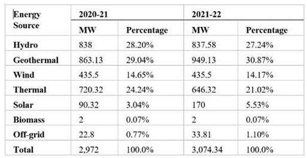
Table 1 shows the Kenya Electricity mix comparison between 2021 and 2022. It shows a steady rise in uptake of renewable energy sources with a decline in the use of thermal power plants in the national grid. The uptake of solar power into the national grid increased significantly from 3% to 5.5% between 2021 and 2022. The government's commitment to diversify the energy mix and transition to 100% renewable sources has increased investments in wind and solar energy projects. The Lake Turkana Wind Power has significantly contributed to wind energy generation in the country [
6].
While the increased installed capacity of renewable sources has allowed more consumers to be connected to the grid, reliability issues persist due to the intermittent nature of renewable energy. Power outages and higher electricity costs remain challenges to be addressed. The government and distribution bodies continue to explore solutions to ensure a reliable and sustainable energy supply for the country.
As a developing economy, Kenya's energy sector faces challenges in power reliability, system resilience, and overall system performance. While significant progress has been made in reducing power disruptions, grid resilience remains a major challenge. The Energy and Petroleum Regulatory Authority (EPRA) attributes this to aging generating systems and grid networks, as well as the detrimental impact of relying heavily on Renewable Energy Resources (RES), which are subject to weather conditions [
7]. The deployment of RES for clean energy goals has raised concerns about their reliability due to their volatile nature in meeting load demand. However, it is important to recognize that RES can be actively monitored and controlled alongside conventional resources, generation systems, and loads within hybrid Renewable Energy Systems (hRES) [
8]. The development of the Garissa Solar Power plant, supported by the national government, aligns with the goals of improving electricity accessibility and transitioning to RES. It is part of a larger effort to explore and develop other renewable sources such as wind, geothermal, and solar energy.
In this research project, the main goal was to develop a machine learning (ML) based power generation prediction model that can be used to predict the power generation of solar power plants in Kenya. The research study used data collected from Garissa solar power plant in Kenya.
Garissa Solar Power Plant
Garissa County is located in Kenya's northeast region and covers an area of 44,174.1 km2. It shares borders with Somalia to the east, Wajir County to the north, Isiolo County to the northwest, Tana River County to the west, and Lamu County to the south [
9]. The county experiences a semi-arid climate with hot and mostly sunny weather throughout the year and the annual rainfall averages around 275 millimeters. It has two rainy seasons: March to May and October to December, with the latter being shorter [
10]. The temperature ranges from 20-40 degrees Celsius, with the hottest months being September to January. The wind speed varies significantly throughout the year, with the windy half occurring from May to October. The highest average hourly wind speed is observed in August, while December has the lowest. The prevailing winds are from the south between March and November and from the east between November and March. The relative humidity fluctuates wildly, with high humidity from September to June and lower humidity in August.
2 Forecasting Techniques
Mamun et al. discuss forecasting techniques to predict future outcomes based on historical data and other relevant factors [
11]. These techniques provide stakeholders with insights into future predictions by analyzing trends. Demand forecasting, a specific type, predicts future product demand by examining current and future consumption and determining the quantity to be supplied [
12]. Forecasting has evolved from simple methods like observing the weather and animal behavior to using sophisticated models and computers to predict temperatures and rainfall probabilities accurately. Forecasting has become crucial in decision-making and planning for minimizing risks and maximizing utilities, especially for planners, investors, and managers [
13] [
14]. Time series forecasting, which focuses on identifying current and past data patterns, is commonly used. Stochastic forecasting models utilize probability theory and statistical methods to predict the behavior of systems affected by random fluctuations [
15].
2.1. Stochastic Forecasting Techniques
Stochastic Differential Equations (SDE) are described as equations that incorporate randomness and unpredictability into the forecasting process [
16]. They consider uncertain factors such as market volatility, consumer consumption, regulations, and geopolitics. Autoregressive integrated moving average (ARIMA) is a statistical model that measures events over time. It relies on historical data and trends to predict future outcomes. ARIMA-ANN, a combination of ARIMA and artificial neural network (ANN), improves forecasting accuracy by detecting non-linear patterns [
17]. The Bayesian Filter, specifically the Bayesian network (BN), is a probabilistic technique used for modeling systems under uncertainty. It considers uncertain parameters like building design, consumer behavior, and system robustness. BN has applications in wind energy modeling, power output forecasting, energy consumption forecasting, and maintenance decision-making [
18]. Geometric Brownian Motion (GBM) is a continuous-time process commonly used in finance to model asset price dynamics. It assumes a constant drift and volatility over time [
19]. GBM has been applied to modeling electricity consumption and simulating price analysis in the energy sector (1).
Where:
µ: drift coefficient
σ: Volatility coefficient
Bt: Brownian motion
Li and Djauhari conducted a study in Malaysia using GBM to model electricity consumption. Their findings showed that the GBM model outperformed the ARIMA model regarding mean absolute percentage error and modeling running time [
20]. This indicates that the GBM approach is more effective in taking into account energy usage. Additionally, Wang and colleagues indicated that GBM is suitable for simulating charge evaluation and determining the flexibility of electric power [
21].
2.2. Machine Learning Forecasting Techniques
2.2.1. Linear Regression
Through linear regression, which is a statistical method that fits dependent and independent variables, it is possible to pick out relationships and patterns among variables and make predictions based on established line. Observation by Ciulla and D'Amico [
22] holds that the usage of more than one linear regression (MLR) for predicting the strength performance of homes emphasizes its accuracy in forecasting and constructing overall performance. However, the findings also acknowledge boundaries, such as the belief of linearity and the requirement of a big dataset for progressed accuracy.
Where:
ŷ = predicted output
β0, β1 =coefficients
x = input
ϵ = error
2.2.2. Decision Tree Regressor
The is a supervised ML technique that make use of a tree structure in predicting the future data based on determined features. It subdivides a dataset into smaller subsets and gradually constructs a decision tree representing the relationships between the features and the predicted outcomes [
23]. The resulting decision tree incorporates decision nodes and leaf nodes, providing a transparent and interpretable framework for making predictions.
2.2.3. Random Forest Algorithm
This algorithm combines multiple decision tress by dividing input parameters into subsets and selection trees which are constructed using the features from each subset [
24]. The algorithm improves of the predictions accuracy through harnessing the collective decision making abilities of the trees.
2.2.4. K–Nearest Neighbors Regression
Considering all available instances, the algorithm uses a similarity metric to predict the numerical target. It selects a specific point and examines its "k" neighbors to determine similarities. By calculating regression for the dataset, the algorithm considers the chosen number of nearest neighbors and averages their results to provide an estimated outcome [
25]. Additionally, the algorithm applies a classification method, categorizing test instances based on their proximity to a predefined set of k-class centers, determined by their features [
24]. Distance measures like Minkowski, Euclidean, or Manhattan distance determine the closeness between models and centers.
Where:
v = class label;
yi = class label of ith nearest neighbors;
I = function returning 1 or 0 for true and false arguments.
2.2.5. Artificial Neural Networks (ANN)
ANN is an ML approach inspired by the structure and functionality of the human brain. It consists of interconnected artificial neurons, or nodes, arranged in three layers: input, hidden, and output. The goal of regression ANNs is to predict an output variable based on the input variables. Designing an artificial neural network (ANN) involves defining distinct hyperparameters, including the quantity of hidden layers, the nodes contained within each layer, and the learning rate. These factors collectively exert significant influence on the network's overall performance [
26]. To obtain optimal performance, the values of these hyperparameters were tweaked using cross-validation. The outcomes of Lu et al. [
27] and Elsheikh et al. [
28] demonstrated the approach's ability to improve building energy efficiency and reduce energy consumption.
2.2.6. Recurrent Neural Networks
RNN is an ANN with the unique characteristic of allowing connections between nodes to form cycles. The core concept underlying RNNs involves retaining the output of a particular layer and feeding it back as input, empowering the network to make predictions based on its previous outputs [
29]. Within the RNN architecture, several hyperparameters are to be specified, including the quantity of recurrent layers, the number of units within each layer, and the learning rate. When predicting solar radiation, the RNN model employs historical data and different meteorological factors [
30]. Findings indicate that the model demonstrates improved prediction accuracy and reduces solar energy system design and operation errors.
2.2.7. Extreme Gradient Boosting (XGBoost) Regression
The XGBoost algorithm is a boosting algorithm that is particularly effective in handling large datasets and making highly accurate predictions. By leveraging these estimators, the algorithm aims to enhance prediction accuracy.
Where:
L(θ) = l(ŷ_i,y_i) and Ω(θ)= γT+ 1/2 λ〖||w||〗^2
Given:
F_obj (θ) = objective function;
L(θ) = loss function;
Ω(θ) = regulation term;
ŷ_i = prediction;
y_i = real value;
T = number of tree leaves;
λ = regulation parameter;
γ = learning rate; and
w = weights of the leaves.
Singh et al. state that the Xgboost regression algorithm can optimize wind power production and reduce greenhouse gas emissions by utilizing historical data and meteorological parameters [
31]. Similarly, Wang et al. found that the Xgboost algorithm's ability to handle non-linear relationships and large datasets is valuable for optimizing energy consumption and reducing costs in industrial settings, particularly for short-term and load forecasting of industrial customers [
31].
2.3. Empirical Research
Accurate prediction of solar Photovoltaic (PV) energy is essential for effective resource planning and participation in energy markets. Various techniques have been explored for forecasting PV solar power, including statistical methods, machine learning techniques, physical models, and hybrid approaches [
32]. Traditional methods face limitations in establishing connections and uncovering implicit information from limited data. Accurate energy forecasting allows energy providers to optimize production schedules, grid operators to manage energy flow and prevent blackouts, and facilitates the integration of renewable energy sources into the power grid [
31]. Forecasting relies on historical data, meteorological conditions, and energy output, with hybrid models combining statistical and physical modeling approaches [
32]. Challenges include the unpredictable nature of weather patterns, the need for extensive data collection, especially in underdeveloped countries, and the complexity and maintenance costs of forecasting models due to the complex behavior of energy systems [
33].
3. Methods and Materials
Electricity generation from solar PV is a factor of various variables in solar plants and environmental factors. Solar irradiance, a crucial factor for solar electricity output, is influenced by location, time of day, season, and weather conditions [
34]. Factors such as wind speed, temperature, and humidity also affect the performance of solar panels by influencing the efficiency of the cells and the accumulation of dust and pollutants on their surface [
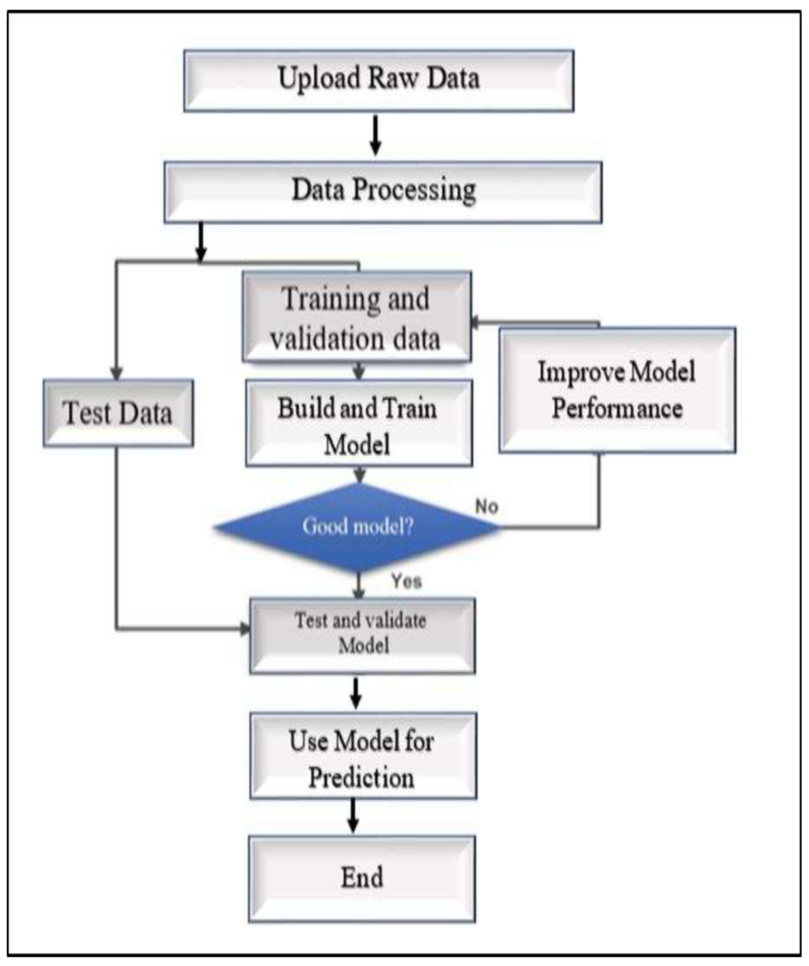
35]. In this research, multiple models were developed using selected ML algorithms for prediction, and their performance was evaluated using model evaluation metrics. The best-performing model was then selected for energy forecasting using forecasted weather data. The flowchart in
Figure 1 outlines the steps used in developing energy prediction models.
The study used three years of data collected from Kenya's Garissa solar power plant. REREC, which is responsible of the plant's commissioning and operation, provided the data. The variables studied included hourly power generation during a three-year period as well as environmental variables such as irradiance, humidity, wind speed, and temperature. The plant is made up of five interconnected modules that work together to generate a single output to the low-voltage transformer. Cleaning the data, arranging the features and labels for training, and separating the data into training and testing sets were all part of the data preprocessing stage.
The data was uploaded to the Collab platform and processed accordingly. The model-building process took place on the Collab platform using the TensorFlow library. The model architecture was created and configured. The next step was training, validating, and testing the model using 60% of the data for training,20% for validation 20% for testing. To evaluate the models, various metrics were utilized, including the coefficient of determination (R2), Mean Absolute Error (MAE), and Root Mean Squared Error (RMSE) [
35]. These metrics assess the performance and accuracy of the model. The models were ranked based on the evaluation results, and the best-performing model was selected for energy generation forecasting.
4. Results and Discussions
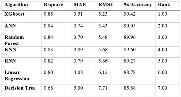
The study compared the performance of seven machine learning (ML) algorithms that were selected from literature These models include; Xgboost, ANN, RNN, KNN, Decision Tree, Random Forest, and Linear Regression. The models were evaluated using metrics such as RMSE, MAE, and R2 scores. The results showed that the Xgboost model had the highest accuracy, with an accuracy rate of 90.42% in predicting power output. It achieved an R2 value of 0.85 and a MAE of 3.50 kW as shown in
Table 2.
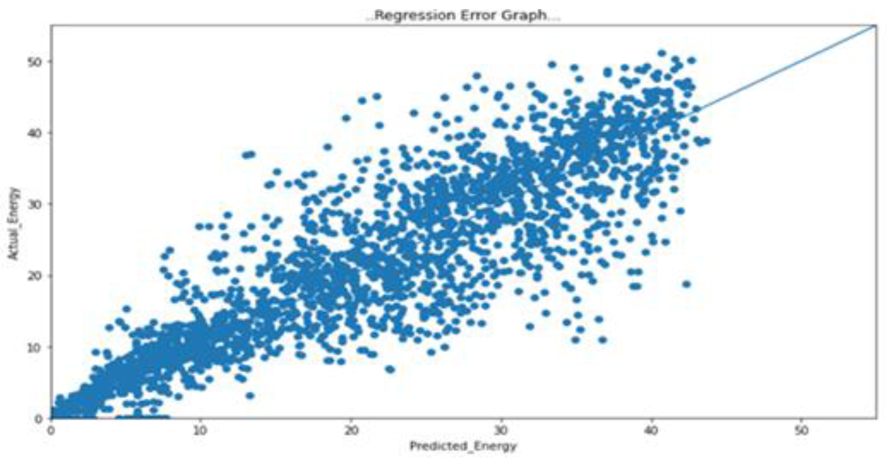
A scatter graph of the actual energy generated vs. the predicted energy data was plotted, as shown in
Figure 2 to ascertain the regression pattern for simplifying analysis.
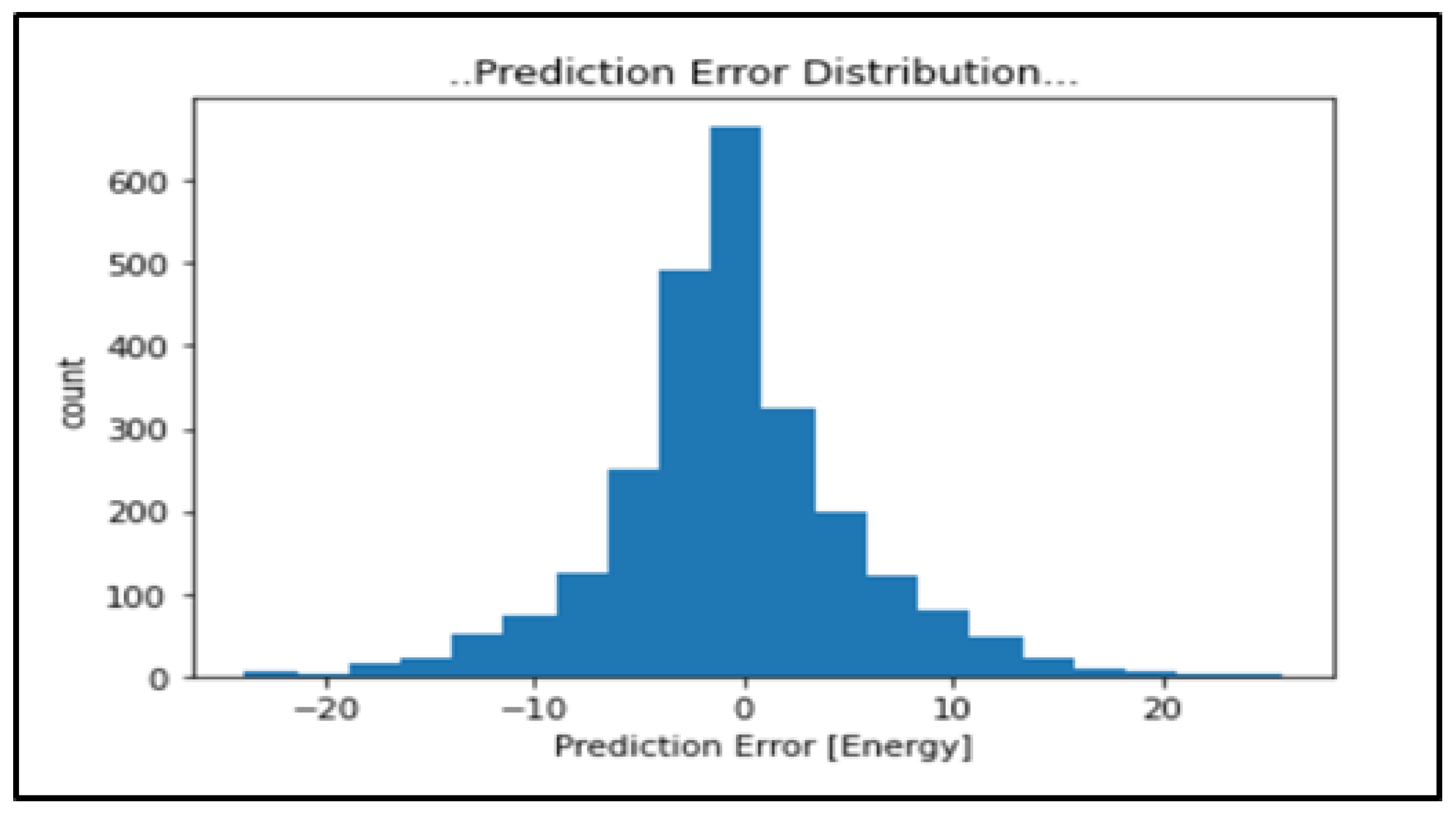
The scatter plot analysis demonstrates a linear relationship between the predicted and actual generated energy. The points on the graph cluster tightly together, indicating a high degree of correlation and a strong relationship between the expected and caused energy values. This suggests that the predictions closely align with the actual energy production. The prediction accuracy plot, displayed as a unimodal symmetrical histogram, indicates that the predicted and actual data were mainly very close, with minimal differences. This shows a high level of accuracy in the predictions, further reinforcing the model's reliability. We can examine and acquire an insight into the efficacy of the models in properly estimating energy generation for the solar power plant by using these visualization tools.
Figure 3 depicts the model’s predicted accuracy distribution. This shows a unimodal symmetrical histogram. This indicated that the difference between predicted and actual data was usually close to zero. It means that the predicted energy was close to the actual generated energy in most instances, indicating that the model can be used to make reliable predictions.
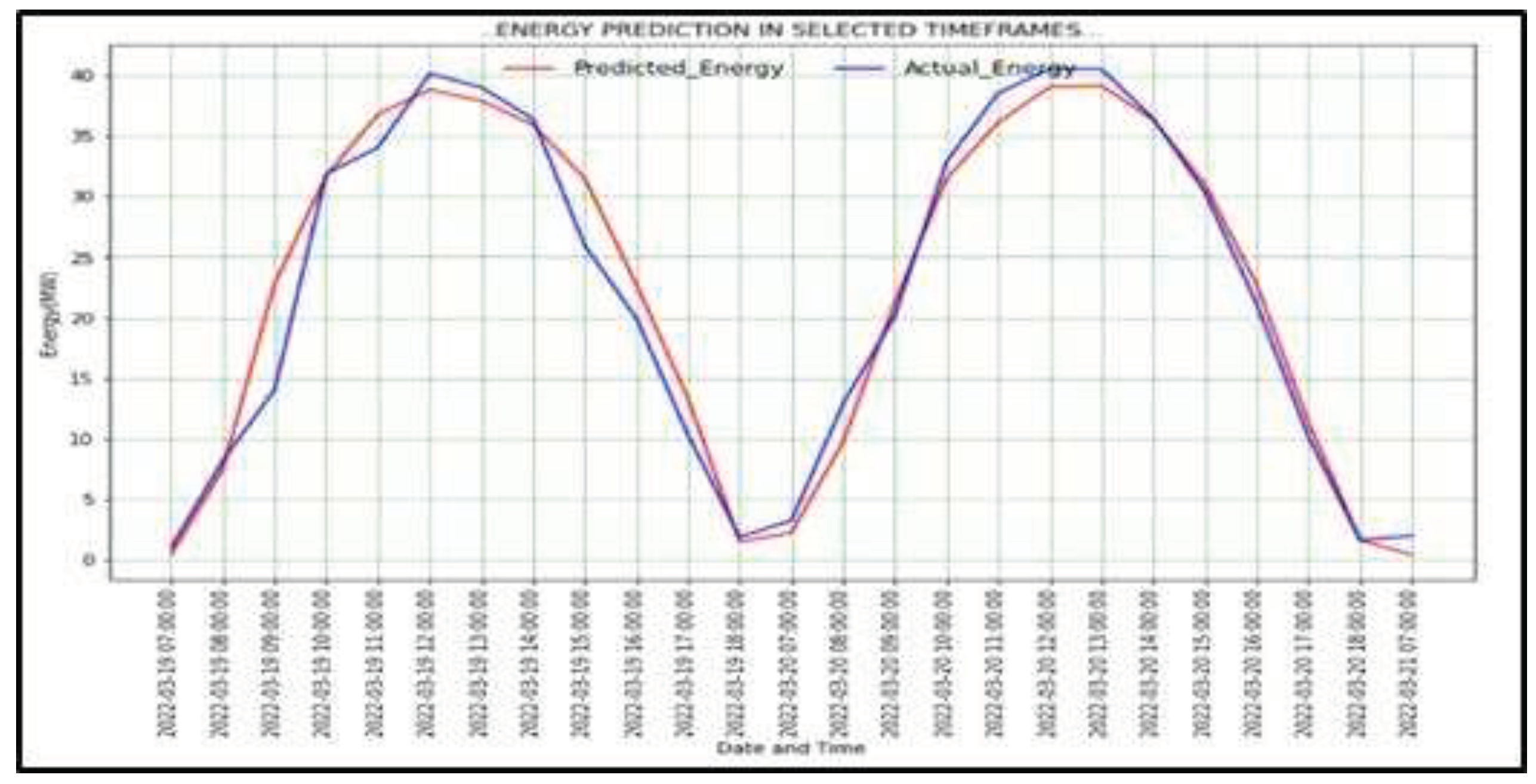
The predicted energy was then plotted against the actual generated data. The plot shows that there was a similarity between the predicted and actual generated energy as shown in
Figure 4.
Discussions
The findings of this study reveals that using weather and operational information as input, accurate power output predictions for the Garissa Solar Power Plant may be obtained. The XGBoost algorithm predicted power output with a high accuracy rate of 90.42%. Because of fluctuating weather conditions and inadequate data, XGBoost's robustness in dealing with missing data and outliers contributed to its accuracy [
31]. This study emphasizes the larger potential of machine learning (ML) in renewable energy, where precise power output prediction is critical for grid stability and reliability.
Other research has focused on the effect of input features, ML method selection, dataset size, and prediction horizon length on the accuracy of ML models in energy prediction [
31]. It is critical for accurate predictions to select important and less noisy input information. Weather, building attributes, and generated electricity all have a substantial impact on model performance [
36] [
37]. In numerous research, various ML methods such ANN, KNN, random forest, SVR, and MLR have been examined [
31]. The performance of various methods varies depending on the properties of the dataset, with ANN frequently outperforming others due to its capacity to handle huge and complex datasets.
ML techniques like as LSTM, SVR, and XGBoost have also been studied in terms of predicting energy use and solar power output. LSTM has exhibited greater accuracy in time-series data handling, whereas XGBoost has demonstrated good accuracy and efficient training time [
38]. The precision of machine learning-driven prediction models is established through the quality and accessibility of data, alongside the intricacy of the model's structure. Only correct and complete data can lead to reasonable forecasts, highlighting the significance of ongoing monitoring, validation, and model modification as new data becomes available.
Accurate power output prediction enables real-time system performance optimization. Operators can make informed decisions based on expected power output, such as altering solar panel tilt angles or activating backup power sources [
39]. Accurate power generation forecasting also supports power generation firms in practical operation and maintenance planning. In solar irradiance, electricity generation, and load forecasting, ML models, particularly Xgboost, have demonstrated improved accuracy and lower prediction errors [
31] [
40]. In addition, ML models have been used to increase the accuracy and reliability of battery management systems, with regression models and deep learning neural network designs generating good R2 scores in predicting battery characteristics and building energy usage.
5. Conclusions
Because of their intermittent nature, RES presents some challenges when integrating into grid systems. It is imperative to accurately forecast RES factors for grid integration, reliability, and stability. This research focused on developing a machine learning-based prediction model for power generation at the Garissa Solar Power Plant in Kenya. Data from the plant, including temperature, humidity, windspeed, irradiance, and electricity generated over three years, was used to train and test seven machine learning algorithms. Performance evaluation metrics such as MAE, MAPE, and RMSE were used to assess and rank the algorithms. The XGBoost algorithm demonstrated the highest accuracy, with 90.42% prediction accuracy. Other algorithms like Random Forest and RNN also showed good performance. ML algorithms' performance depends on their ability to handle complex datasets, and accurate data is crucial for plant performance and grid stability. Continuous monitoring, validation, and refinement of prediction models are necessary. Aggregated-level energy performance prediction provides more accurate results, enabling real-time adjustments to optimize system performance.
Acknowledgments
The authors would like to express their gratitude to REREC for availing data that was used for the study and to staff members at the Department of Energy Policy and Engineering at KEPCO International Graduate School for their technical assistance and inputs.
Conflicts of Interest
The authors declare no conflict of interest regarding the publication of this paper.
References
- Gore, C. D., Brass, J. N., Baldwin, E., & MacLean, L. M. (2019). Political autonomy and resistance in electricity sector liberalization in Africa. World development, 120, 193-209. [CrossRef]
- Foster, V., Eberhard, A., & Dyson, G. (2022). The evolution of electricity sectors in Africa: ongoing obstacles and emerging opportunities to reach universal targets. Digest of the, 70. [CrossRef]
- Ambani, B. (24-Nov-2022). “Electricity outage hits parts of Kenya as power system fails,” The East African. [Online]. Available: https://www.theeastafrican.co.ke/tea/news/east-africa/kenya-suffers-nationwide-power-outage-4032052.
- Boamah, F., Williams, D. A., & Afful, J. (2021). Justifiable energy injustices? Exploring institutionalised corruption and electricity sector “problem-solving” in Ghana and Kenya. Energy Research & Social Science, 73, 101914. [CrossRef]
- Lima, Y. A. (2023). Renewable energy in Africa: Kenya's success and its possible implementation in Angola. Payne Institute Student Commentary Series: Commentary, 1(1), 1-15. www.trade.gov/country-commercial-guides/kenya-energy-electrical-power-systems#:~:text=Current%20Energy%20Mix%3A%20Kenya's%20energy,thermal%2C%20biomass%2C%20and%20imports.
- Kiplagat, J. K., Wang, R. Z., & Li, T. X. (2011). Renewable energy in Kenya: Resource potential and status of exploitation. Renewable and Sustainable Energy Reviews, 15(6), 2960-2973. [CrossRef]
- Musonye, X. S., Davíðsdóttir, B., Kristjánsson, R., Ásgeirsson, E. I., & Stefánsson, H. (2020). Integrated energy systems’ modeling studies for sub-Saharan Africa: A scoping review. Renewable and Sustainable Energy Reviews, 128, 109915. [CrossRef]
- Wang, X., Palazoglu, A., & El-Farra, N. H. (2015). Operational optimization and demand response of hybrid renewable energy systems. Applied Energy, 143, 324-335. [CrossRef]
- Ogeya, M. C., Osano, P., Kingiri, A., & Okemwa, J. M. (2021). Challenges and opportunities for the expansion of renewable electrification in Kenya. Youba Sokona, Vice-Chair of the Intergovernmental Panel on Climate Change (IPCC), 46. [CrossRef]
- Isako, T., & Kimindu, V. (2019). Camel milk value chain in Kenya: A review. J Marketing Consumer Res, 58, 51-64. https://www.iiste.org/Journals/index.php/JMCR/article/view/48809.
- Al Mamun, A., Sohel, M., Mohammad, N., Sunny, M. S. H., Dipta, D. R., & Hossain, E. (2020). A comprehensive review of the load forecasting techniques using single and hybrid predictive models. IEEE Access, 8, 134911-134939. [CrossRef]
- Petropoulos, F., Apiletti, D., Assimakopoulos, V., Babai, M. Z., Barrow, D. K., Taieb, S. B., ... & Ziel, F. (2022). Forecasting: theory and practice. International Journal of Forecasting, 38(3), 705-871.
- Negnevitsky, M., Mandal, P., & Srivastava, A. K. (2009, July). An overview of forecasting problems and techniques in power systems. In 2009 IEEE Power & Energy Society General Meeting (pp. 1-4). IEEE. [CrossRef]
- Petropoulos, F., Apiletti, D., Assimakopoulos, V., Babai, M. Z., Barrow, D. K., Taieb, S. B., ... & Ziel, F. (2022). Forecasting: theory and practice. International Journal of Forecasting, 38(3), 705-871. [CrossRef]
- Wekesa, D. W., Wang, C., Wei, Y., Kamau, J. N., & Danao, L. A. M. (2015). A numerical analysis of unsteady inflow wind for site specific vertical axis wind turbine: A case study for Marsabit and Garissa in Kenya. Renewable Energy, 76, 648-661. [CrossRef]
- Zhang, X., Xu, Y., Schmalfuß, B., & Pei, B. (2019). Random attractors for stochastic differential equations driven by two-sided Lévy processes. Stochastic Analysis and Applications, 37(6), 1028-1041. [CrossRef]
- Milano, F., & Zárate-Miñano, R. (2013). A systematic method to model power systems as stochastic differential algebraic equations. IEEE Transactions on Power Systems, 28(4), 4537-4544. [CrossRef]
- Adedipe, T., Shafiee, M., & Zio, E. (2020). Bayesian network modelling for the wind energy industry: An overview. Reliability Engineering & System Safety, 202, 107053. [CrossRef]
- Noel, K. (2019). Neural Stochastic Control Application: Optimal Portfolio Allocation. Available at SSRN 3420201. [CrossRef]
- Jakaša, T., Andročec, I., & Sprčić, P. (2011, May). Electricity price forecasting—ARIMA model approach. In 2011 8th International Conference on the European Energy Market (EEM) (pp. 222-225). IEEE.
- Siami-Namini, S., Tavakoli, N., & Namin, A. S. (2018, December). A comparison of ARIMA and LSTM in forecasting time series. In 2018 17th IEEE international conference on machine learning and applications (ICMLA) (pp. 1394-1401). IEEE.
- Tamer, T., Dino, I. G., & Akgül, C. M. (2022). Data-driven, long-term prediction of building performance under climate change: Building energy demand and BIPV energy generation analysis across Turkey. Renewable and Sustainable Energy Reviews, 162, 112396. [CrossRef]
- Osisanwo, F. Y., Akinsola, J. E. T., Awodele, O., Hinmikaiye, J. O., Olakanmi, O., & Akinjobi, J. (2017). Supervised machine learning algorithms: classification and comparison. International Journal of Computer Trends and Technology (IJCTT), 48(3), 128-138. [CrossRef]
- Ranjbar, S., Farsa, A. R., & Jamali, S. (2020). Voltage-based protection of microgrids using decision tree algorithms. International Transactions on Electrical Energy Systems, 30(4), e12274. [CrossRef]
- Song, Y., Liang, J., Lu, J., & Zhao, X. (2017). An efficient instance selection algorithm for k nearest neighbor regression. Neurocomputing, 251, 26-34. [CrossRef]
- Fei, G., Wang, S., & Liu, B. (2016, August). Learning cumulatively to become more knowledgeable. In Proceedings of the 22nd ACM SIGKDD International Conference on Knowledge Discovery and Data Mining (pp. 1565-1574). [CrossRef]
- Cao, X., Dai, X., & Liu, J. (2016). Building energy-consumption status worldwide and the state-of-the-art technologies for zero-energy buildings during the past decade. Energy and buildings, 128, 198-213. [CrossRef]
- Khandelwal, I., Adhikari, R., & Verma, G. (2015). Time series forecasting using hybrid ARIMA and ANN models based on DWT decomposition. Procedia Computer Science, 48, 173-179. [CrossRef]
- Jozefowicz, R., Zaremba, W., & Sutskever, I. (2015, June). An empirical exploration of recurrent network architectures. In International conference on machine learning (pp. 2342-2350). PMLR.
- Sameen, M. I., & Pradhan, B. (2017). Severity prediction of traffic accidents with recurrent neural networks. Applied Sciences, 7(6), 476. [CrossRef]
- Singh, U., & Rizwan, M. (2022). SCADA system dataset exploration and machine learning based forecast for wind turbines. Results in Engineering, 16, 100640. [CrossRef]
- Wang, H., Lei, Z., Zhang, X., Zhou, B., & Peng, J. (2019). A review of deep learning for renewable energy forecasting. Energy Conversion and Management, 198, 111799. [CrossRef]
- Yazdanie, M., & Orehounig, K. (2021). Advancing urban energy system planning and modeling approaches: Gaps and solutions in perspective. Renewable and Sustainable Energy Reviews, 137, 110607. https://econpapers.repec.org/scripts/redir.pf?u=https%3A%2F%2Fdoi.org%2F10.1016%252Fj.rser.2020.110607;h=repec:eee:rensus:v:137:y:2021:i:c:s1364032120308911. [CrossRef]
- Rajagukguk, R. A., Ramadhan, R. A., & Lee, H. J. (2020). A review on deep learning models for forecasting time series data of solar irradiance and photovoltaic power. Energies, 13(24), 6623. [CrossRef]
- Said, S. A., Hassan, G., Walwil, H. M., & Al-Aqeeli, N. (2018). The effect of environmental factors and dust accumulation on photovoltaic modules and dust-accumulation mitigation strategies. Renewable and Sustainable Energy Reviews, 82, 743-760. [CrossRef]
- Olu-Ajayi, R., Alaka, H., Sulaimon, I., Sunmola, F., & Ajayi, S. (2022). Building energy consumption prediction for residential buildings using deep learning and other machine learning techniques. Journal of Building Engineering, 45, 103406. [CrossRef]
- Al-Shargabi, A. A., Almhafdy, A., Ibrahim, D. M., Alghieth, M., & Chiclana, F. (2022). Buildings' energy consumption prediction models based on buildings’ characteristics: Research trends, taxonomy, and performance measures. Journal of Building Engineering, 54, 104577. [CrossRef]
- Devan, P., & Khare, N. (2020). An efficient XGBoost–DNN-based classification model for network intrusion detection system. Neural Computing and Applications, 32, 12499-12514. [CrossRef]
- Singhal, R., Choudhary, N. K., & Singh, N. (2019). Short-term load forecasting using hybrid ARIMA and artificial neural network model. In Advances in VLSI, Communication, and Signal Processing: Select Proceedings of VCAS 2018 (pp. 935-947). Singapore: Springer Singapore. [CrossRef]
- Aguilar Madrid, E., & Antonio, N. (2021). Short-term electricity load forecasting with machine learning. Information, 12(2), 50. [CrossRef]
|
Disclaimer/Publisher’s Note: The statements, opinions and data contained in all publications are solely those of the individual author(s) and contributor(s) and not of MDPI and/or the editor(s). MDPI and/or the editor(s) disclaim responsibility for any injury to people or property resulting from any ideas, methods, instructions or products referred to in the content. |
© 2023 by the authors. Licensee MDPI, Basel, Switzerland. This article is an open access article distributed under the terms and conditions of the Creative Commons Attribution (CC BY) license (http://creativecommons.org/licenses/by/4.0/).
