Submitted:
18 August 2023
Posted:
18 August 2023
You are already at the latest version
Abstract
Keywords:
1. Introduction
2. Materials and Methods
2.1. Simulation-Based Techniques
- Precision: Simulation models can offer precise predictions when properly calibrated and grounded in real-world data.
- Flexibility: They can be tailored to accommodate diverse scenarios and configurations.
- Understanding: Simulations facilitate comprehension of the intricate interactions between different components within the energy system.
- Computational Intensity: Developing and executing simulations can be computationally demanding, particularly for large-scale systems.
- Data Requirements: High-quality data pertaining to weather, energy demand, and system parameters are crucial for ensuring accurate simulations.
- Complexity: Constructing a reliable simulation model necessitates expertise and domain knowledge.
2.2. AI Predictions for Electricity Generation from RES
- Speed: AI models can rapidly process vast data-sets and provide real-time predictions.
- Adaptability: They possess the ability to adapt to changing conditions and learn from newly acquired data.
- Scalability: AI models demonstrate efficacy in handling large-scale systems.
- Data Quality: The accuracy of AI predictions heavily relies on the quality and sentative character of the training data.
- Black Box Nature: Neural networks can be challenging to interpret, making it difficult to comprehend the underlying reasoning behind predictions.
- Limited Generalization: AI models may encounter difficulties when dealing with unseen situations or data that significantly deviate from the training set.
2.3. Analyzed desgined PV farm
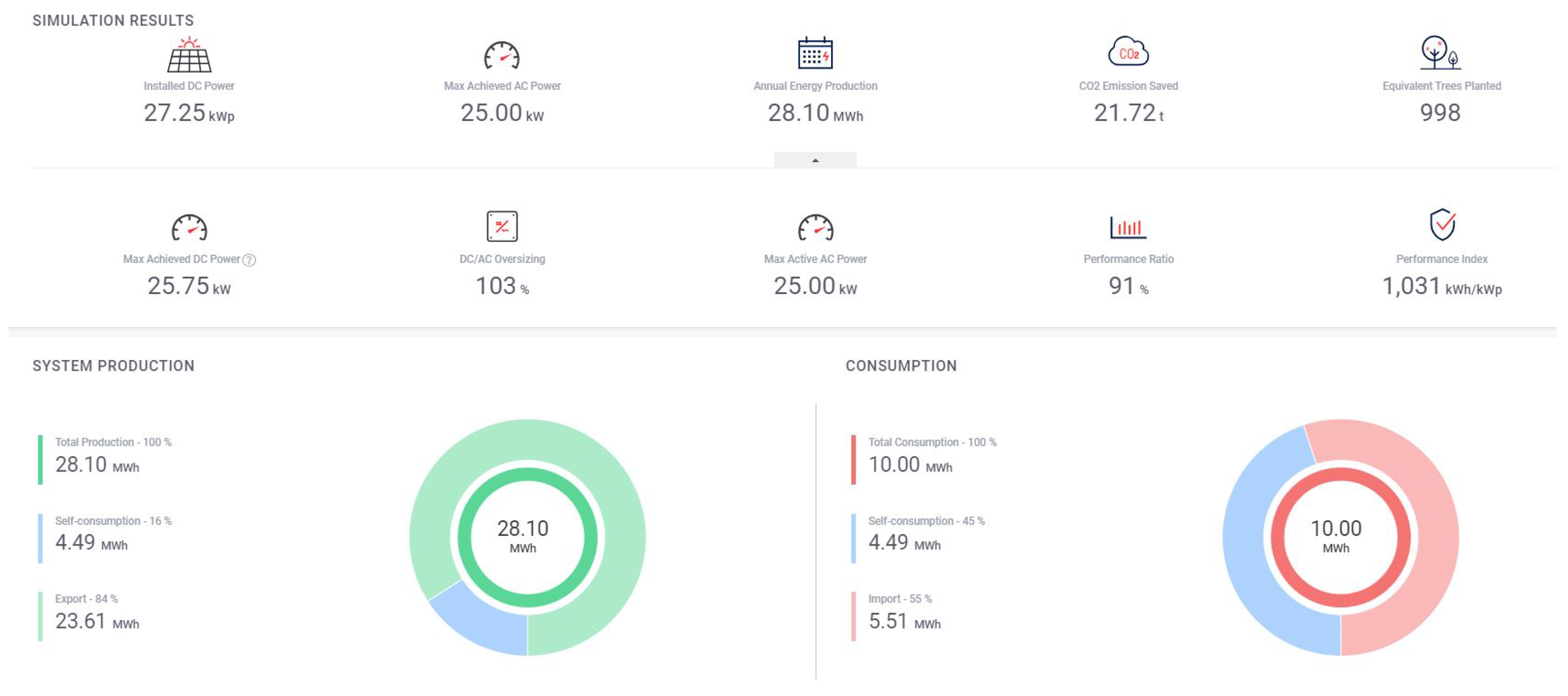
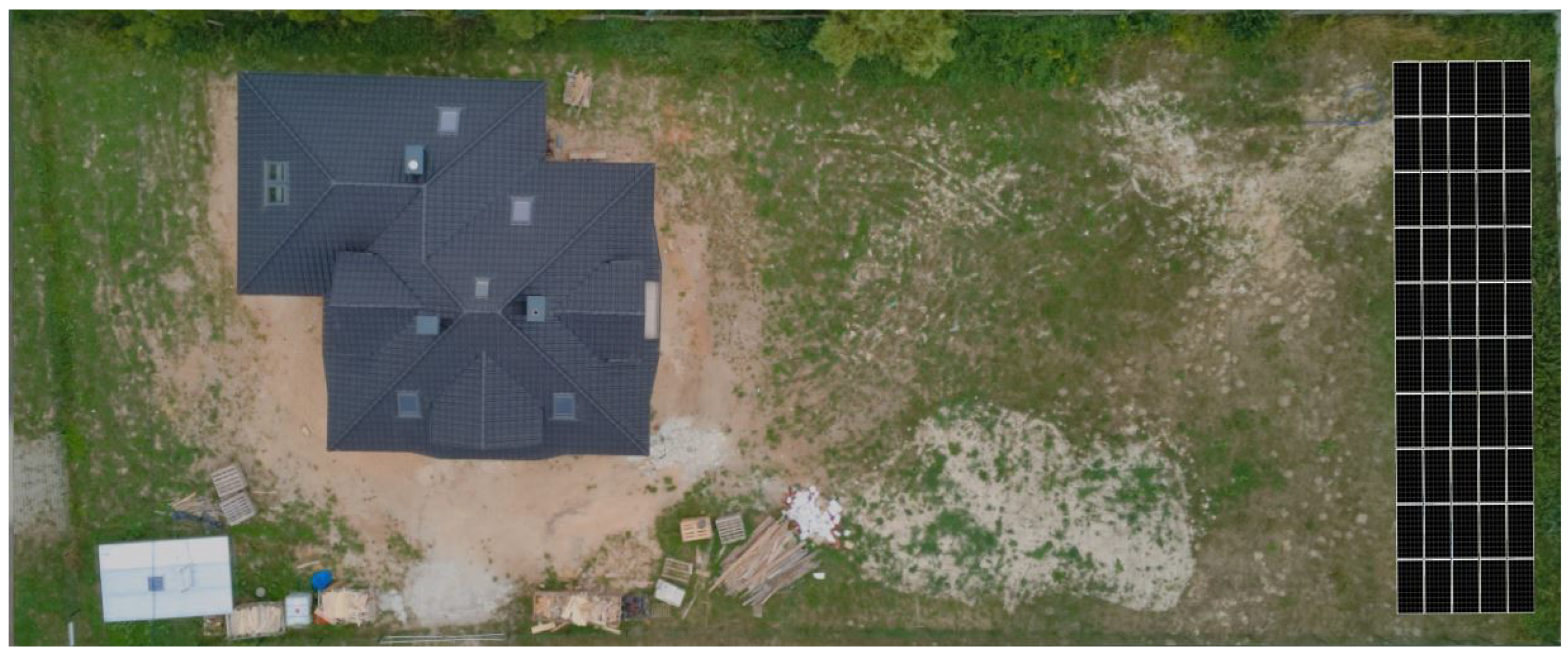
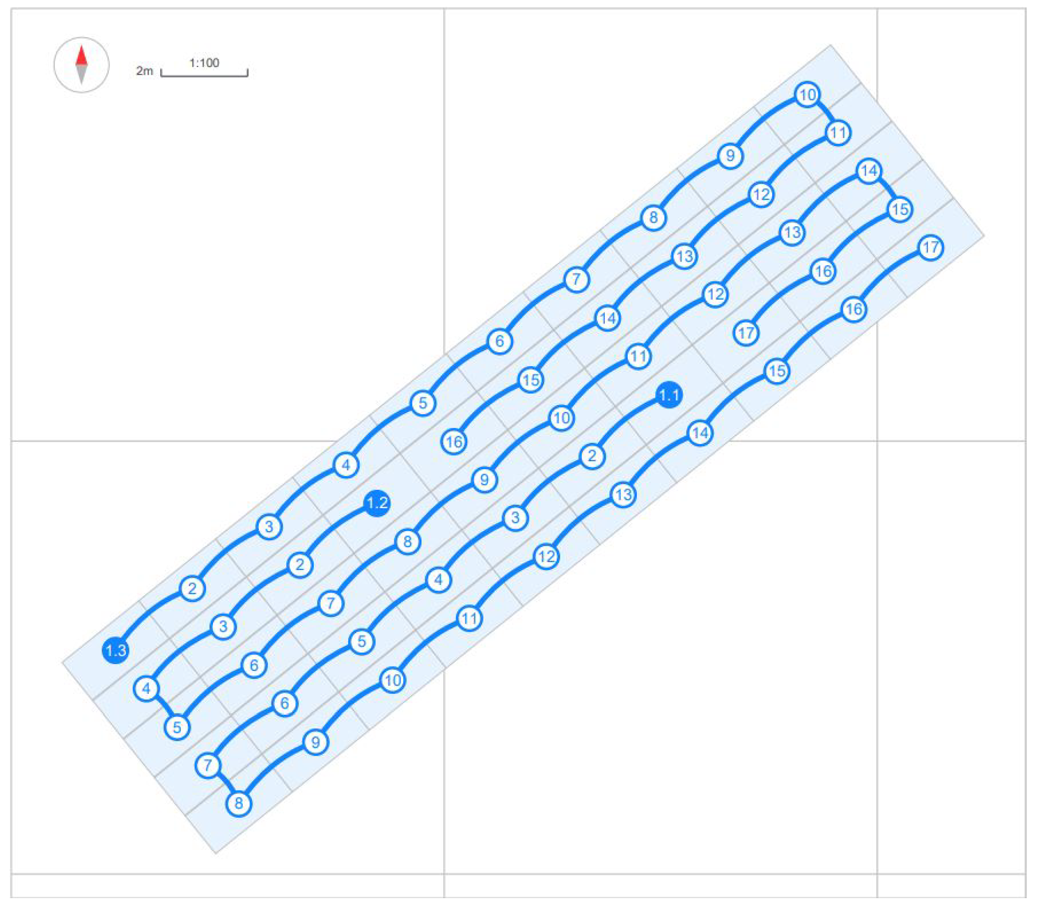
- The PV farm has a total installed DC power capacity of 27.25 kilowatts peak (KWp). This is achieved through the use of 50 JAM72D30-545/MB solar panels.
- The PV system utilizes a Solar Edge SE25K inverter, which has a capacity of 25,000 watts. The inverter converts the DC power generated by the solar panels into AC power, suitable for use in homes and businesses.
- To maximize energy production and improve efficiency, the PV farm is equipped with 50 Solar Edge S650B optimizers. These optimizers individually track and optimize the performance of each solar panel, ensuring that the entire system operates at its highest potential.
- The maximum AC power output of the PV farm is 25 kilowatts (KW). This represents the highest amount of electricity that the system can produce and supply to the grid or connected loads at any given moment.
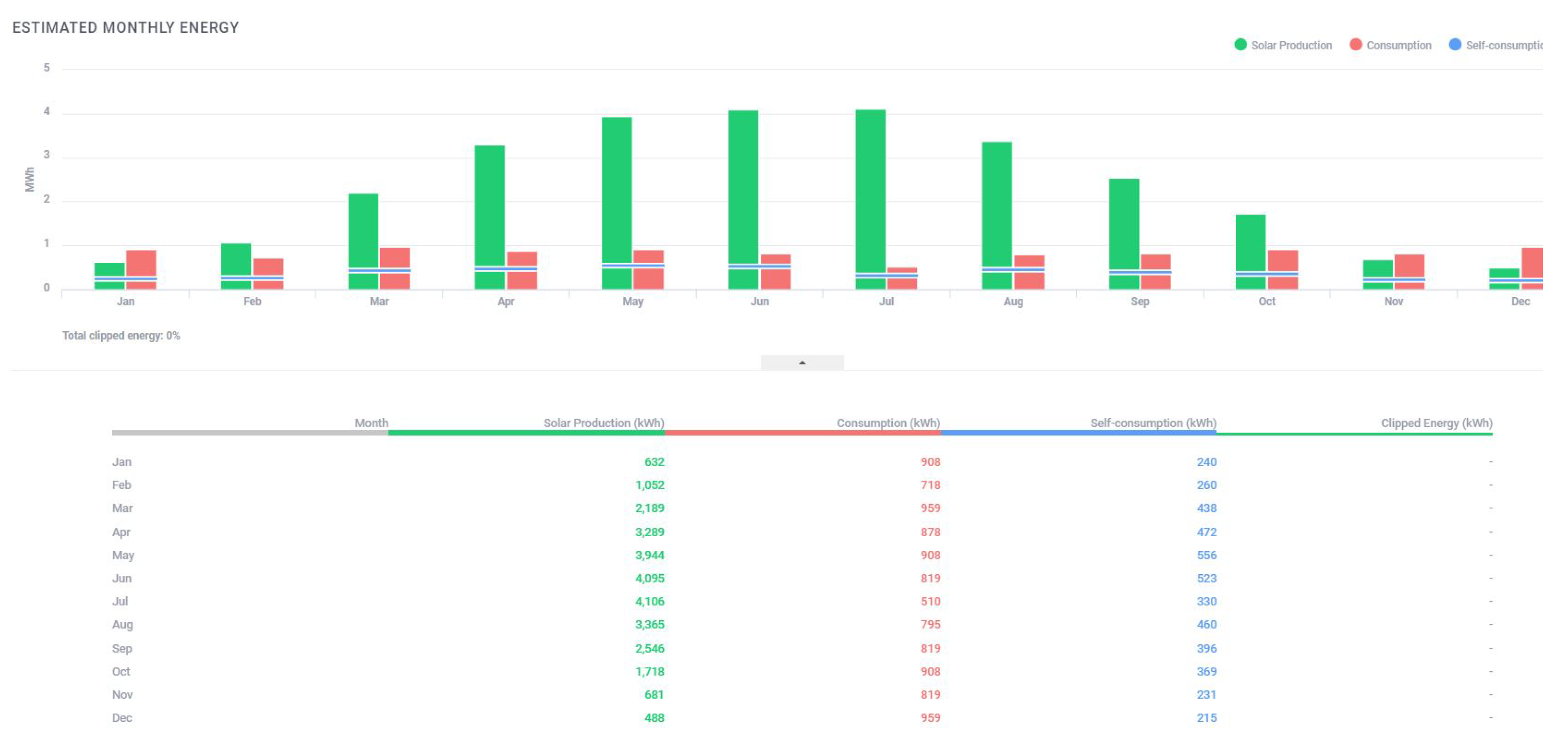
- The PV farm’s estimated annual energy production is 28.10 megawatt-hours (MWh). This figure indicates the total amount of electricity the system is expected to generate over the course of a year under average sunlight conditions.
- The performance index of the PV farm is 91%. This metric represents the efficiency of the system in converting sunlight into electricity. An index of 91 suggests that the PV farm is performing at a high level of efficiency, considering various factors such as shading, temperature, and soiling losses.
2.4. Parameters used as input for DNN
- Timestamp: The date and time at which the data is recorded, providing a temporal context for the other parameters.
- Global Horizontal Irradiance: The total solar irradiance received on a horizontal surface, including direct and diffuse sunlight.
- Diffuse Horizontal Irradiance: The solar irradiance from the sky’s scattered radiation received on a horizontal surface.
- Diffused Normal Irradiance: The solar irradiance received on a surface perpendicular to the sun’s rays, after scattering in the atmosphere.
- Global Tilted Irradiance: The total solar irradiance received on a tilted surface, which is typically the PV panel’s orientation.
- Temperature: The ambient temperature of the solar PV panels or system.
- GTI Loss: Loss in Global Tilted Irradiance, potentially due to shading or orientation issues.
- Irradiance Shading Loss: Loss in irradiance due to shading on the PV panels.
- Array Incidence Loss: Loss caused by the angle at which sunlight strikes the PV panels.
- Soiling and Snow Loss: Loss due to the accumulation of dirt, dust, or snow on the PV panels, reducing their efficiency.
- Nominal Energy: The expected energy output from the PV system under ideal conditions.
- Irradiance Level Loss: Loss related to variations in solar irradiance levels.
- Shading Electrical Loss: Electrical losses occurring in the system due to shading.
- Temperature Loss: Electrical losses caused by temperature variations in the PV panels.
- Optimizer Loss: Losses associated with power optimizers used in the PV system.
- Yield Factor Loss: Losses due to factors impacting the system’s overall yield.
- Module Quality Loss: Losses caused by the quality of PV modules used in the system.
- LID Loss: Light-Induced Degradation losses in PV modules.
- Ohmic Loss: Electrical losses caused by the resistance of materials in the system.
- String Clipping Loss: Losses due to limiting the output of strings of PV panels.
- Array Energy: The total energy output from the PV array.
- Inverter Efficiency Loss: Losses due to inefficiencies in the inverter.
- Clipping Loss: Losses due to limiting the system’s output to protect the inverter.
- System Unavailability Loss: Losses due to system downtime or unavailability.
- Export Limitation Loss: Losses caused by limitations on exporting excess energy to the grid.
- Battery Charge: The amount of energy being charged into the battery storage system.
- Battery Discharge: The amount of energy being discharged from the battery storage system.
- Battery State of Energy: The current energy level or state of charge of the battery.
- Inverter Output: The energy output from the inverter.
- Consumption: The amount of energy consumed by the user or load.
- Self-consumption: The energy consumed from the PV system by the user.
- Imported Energy: The amount of energy imported from the grid.
- Exported Energy: The amount of excess energy exported to the grid.
3. Results
- MAE (Mean Absolute Error): 98.531 The MAE represents the average absolute difference between the predicted values and the actual values. In this case, the average absolute error is 98.531, which means, on average, the predictions made by the DNN are off by approximately 98.531 Kwh.
- NMAE (Normalized Mean Absolute Error): 0.048 NMAE is the MAE normalized by the mean of the actual values. It is a relative measure of the MAE and is useful for comparing performance across different data-sets. In this case, the NMAE is 0.048, indicating that the DNN’s predictions have an average absolute error of 4.8% relative to the mean of the actual values.
- MPL (Mean Percentage Loss): 49.265 The MPL represents the average percentage difference between the predicted values and the actual values. In this case, the average percentage loss is 49.265, which means, on average, the predictions made by the DNN deviate from the actual values by approximately 49.265%.
- MAPE (Mean Absolute Percentage Error): 0.085 MAPE is a common metric for measuring the accuracy of predictions as a percentage. It represents the average absolute percentage difference between the predicted values and the actual values. In this case, the average absolute percentage error is 0.085, meaning that the DNN’s predictions have an average error of 8.5% relative to the actual values.
- MSE (Mean Squared Error): 18724.956 The MSE represents the average of the squared differences between the predicted values and the actual values. It gives higher weights to larger errors. In this case, the MSE is 18724.956, providing an insight into the average squared error of the DNN’s predictions.
- EVS (Explained Variance Score): 0.889 EVS measures the proportion of variance in the target variable that is explained by the model. It ranges from 0 to 1, where 1 indicates a perfect fit. An EVS of 0.889 means that the DNN explains about 88.9% of the variance in the data, which is considered a good result.
- R2 (R-squared): 0.867 R-squared is another measure of how well the model fits the data. It represents the proportion of variance in the target variable that can be predicted from the input features. R-squared also ranges from 0 to 1, with 1 indicating a perfect fit. An R2 value of 0.867 indicates that the DNN explains about 86.7% of the variance in the data.
- RMSE (Root Mean Squared Error): 136.839 RMSE is the square root of the MSE and is a common metric for evaluating the accuracy of predictions. It represents the average magnitude of the errors made by the DNN. In this case, the RMSE is 136.839, providing an insight into the average magnitude of the errors made by the DNN’s predictions.
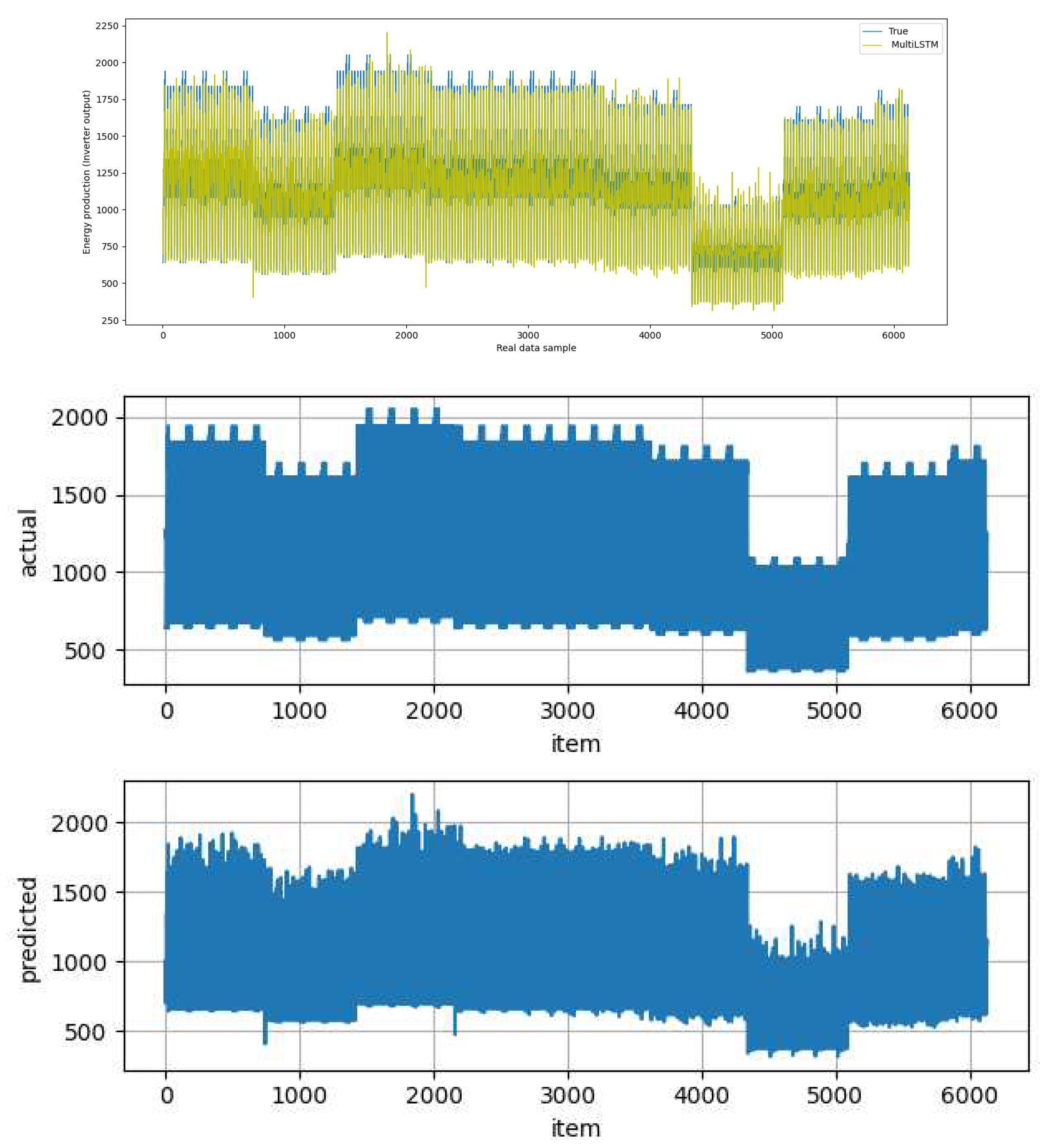
| MAE: 98.531 | NMAE: 0.048 | MPL: 49.265 |
| MAPE: 0.085 | MSE: 18724.956 | |
| EVS: 0.889 | R2: 0.867 | RMSE: 136.839 |
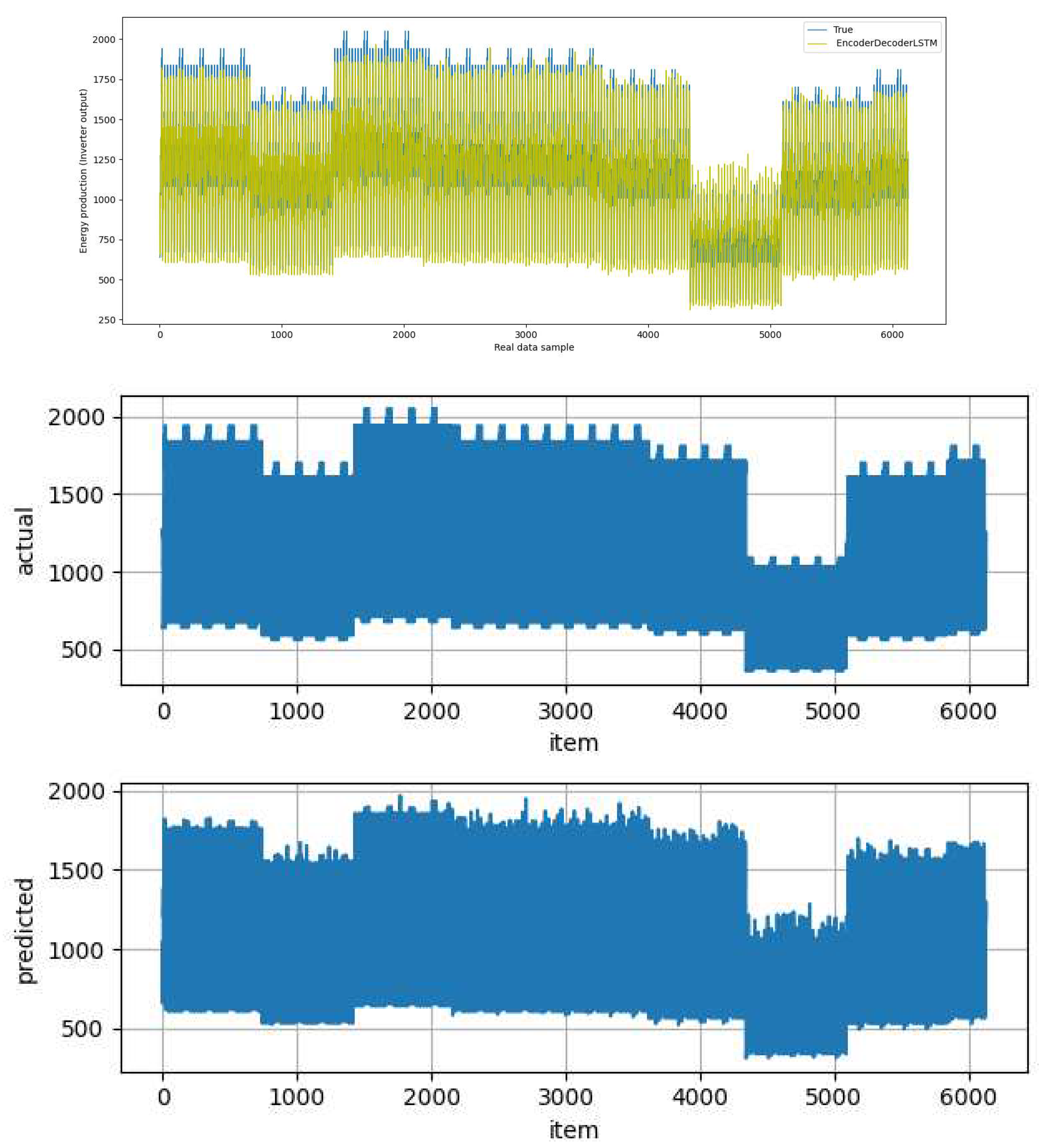
| MAE: 130.454 | NMAE: 0.063 | MPL: 65.227 |
| MAPE: 0.124 | MSE: 29203.207 | |
| EVS: 0.826 | R2: 0.805 | RMSE: 170.889 |
- Mean Absolute Error (MAE): The MAE is measured at approximately 130.454 KWh, indicating the average discrepancy between predicted and actual values.
- Normalized Mean Absolute Error (NMAE): The NMAE stands at around 0.063, representing the relative average absolute error.
- Mean Absolute Percentage Error (MAPE): The MAPE is about 0.124%, signifying the average error as a percentage of the actual values.
- Mean Squared Error (MSE): The MSE is approximately 29203.207, reflecting the average squared difference between predicted and actual values.
- Explained Variance Score (EVS): With a value of approximately 0.826, the EVS suggests a reasonably good fit of the model to the data. An EVS close to 1 indicates a stronger fit.
- Coefficient of Determination (R2): The R2 value is estimated at around 0.805, which serves as a measure of the model’s accuracy in explaining the variance in the dependent variable.
- Root Mean Squared Error (RMSE): The RMSE is evaluated at approximately 170.889 KWh, signifying the square root of the average squared error.
4. Discussion
References
- Demirkiran, Muhammet and Karakaya, Abdulhakim. "Efficiency analysis of photovoltaic systems installed in different geographical locations" Open Chemistry 20, no. 1 (2022): 748-758. https://doi.org/10.1515/chem-2022-0190. [CrossRef]
- Roberts, J.; Cassula, A.; Freire, J.; Prado, P. Simulation and Validation Of Photovoltaic System Performance Models. In Proceedings of the XI Latin-American Congress on Electricity Generation and Transmission–CLAGTEE 2015, Sao Paulo, Brazil, 8–11 November 2015.
- Milosavljević, D.D.; Kevkić, T.S.; Jovanović, S.J. Review and validation of photovoltaic solar simulation tools/software based on case study. Open Phys. 2022, 20, 431–451. [CrossRef]
- Jaroslaw Bilski, Leszek Rutkowski, Jacek Smolag, Dacheng Tao: A novel method for speed training acceleration of recurrent neural networks. Inf. Sci. 553: 266-279 (2021). [CrossRef]
- Bochenek, B.; Jurasz, J.; Jaczewski, A.; Stachura, G.; Sekuła, P.; Strzyżewski, T.; Wdowikowski, M.; Figurski, M. Day-Ahead Wind Power Forecasting in Poland Based on Numerical Weather Prediction. Energies 2021, 14, 2164. https://doi.org/10.3390/en14082164. [CrossRef]
- Shao, X.; Kim, C.-S.; Sontakke, P. Accurate Deep Model for Electricity Consumption Forecasting Using Multi-Channel and Multi-Scale Feature Fusion CNN–LSTM. Energies 2020, 13, 1881. https://doi.org/10.3390/en13081881. [CrossRef]
- Jabreel, Mohammed & Moreno, Antonio. (2019). A Deep Learning-Based Approach for Multi-Label Emotion Classification in Tweets. Applied Sciences. 9. 1123. 10.3390/app9061123. [CrossRef]
Disclaimer/Publisher’s Note: The statements, opinions and data contained in all publications are solely those of the individual author(s) and contributor(s) and not of MDPI and/or the editor(s). MDPI and/or the editor(s) disclaim responsibility for any injury to people or property resulting from any ideas, methods, instructions or products referred to in the content. |
© 2023 by the authors. Licensee MDPI, Basel, Switzerland. This article is an open access article distributed under the terms and conditions of the Creative Commons Attribution (CC BY) license (http://creativecommons.org/licenses/by/4.0/).


