Preprint
Article

A New Optimization Design Method of Multi-Objective Indoor Air Supply Using Kriging Model and NSGA-II

Altmetrics

Downloads

68

Views

24

Comments

0

A peer-reviewed article of this preprint also exists.

This version is not peer-reviewed

Submitted:

18 August 2023

Posted:

21 August 2023

You are already at the latest version

Alerts
Abstract
When using meta-heuristic optimization approaches for optimization, a large number of samples are required. In particular, when generating subgeneration, the utilization of existing samples is low and the number of individuals is high. Therefore, surrogate-based optimization has been developed, which greatly reduces the number of individuals in the subgeneration and the cost of optimization. In complex air supply scenarios, single-objective optimization results may not be comprehensive; therefore, this paper developed a double-objective air supply optimization method based on the Kriging surrogate model and Non-dominated Sorting Genetic Algorithms-II. And proposed the infill criteria based on clustering to advance the Pareto Frontier. The method was validated by an inverse prediction case, and in particular, the problems when based on 3D steady-state simulations were analyzed. The results showed that the method can quickly achieve an approximate prediction of the boundary conditions (when prediction were made based on experimental data, the number of simulations was 82 and the average error was 6.8%). Finally, the method was used to optimize the air supply parameters of a dual-aisle, single-row cabin. The Pareto set suggested that an airflow organization with dual circulation may be optimal.
Keywords: 
Subject: Engineering  -   Architecture, Building and Construction

1. Introduction

When designing air supply systems to create a comfortable environment, the design of air supply parameters is a very critical part of the process. Inverse design is currently a more effective design method than trial-and-error methods, where only forward methods (including the CFD-based adjoint method [1,2], the CFD-based genetic algorithm method [3,4], the Proper orthogonal decomposition (POD) method [5], etc.) can be used to design the desired air environment, and the reverse methods can be used for traceability [6]. The above forward methods are based on the results obtained under known parameter combinations, combined with some methods to determine new parameter combinations, continuously verify and improve, and finally get the parameter combinations that meet the design objectives. For example, the CFD-based adjoint method can be used to obtain the partial derivatives of the dependent variable by computational fluid dynamics (CFD) to produce the next parameters combination. The CFD-based genetic algorithm method, on the other hand, is a non-gradient-based optimization method that inherits the advantages and disadvantages of evolutionary algorithms. The POD method is based on interpolation prediction, and its accuracy depends entirely on the interpolation accuracy [7].
In fact, the forward air supply optimization design is a multi-parameter optimization process, where the optimization variables are the air outlet design parameters and the optimization targets are the full design requirements. Existing optimization methods are generally classified into two main categories: gradient-based optimization methods and non-gradient-based optimization methods. Gradient-based methods do not handle nonlinear problems well and are easily trapped in local optima [8,9]. While the Navier-Stokes equations are highly nonlinear, global optimization often requires the use of non-gradient-based meta-heuristic optimization approaches (a series of general-purpose heuristic optimization approaches) such as genetic algorithm [10], differential evolution algorithm [11], simulated annealing [12], particle swarm optimization (PSO) [13], sequential quadratic programming [14] etc. Based on these algorithms, various types of algorithms have been developed to optimize single-objective and multi-objective problems, and a mixture of them is also an effective strategy in practical optimization applications, such as the combination of simulated annealing and particle swarm optimization [15].
In this paper, the authors have compiled some of the newest studies, as shown in Table 1. It can be found that studies based on meta-heuristic optimization approaches and meta-heuristic optimization approaches combined with artificial neural networks are mainstream in air supply design, air conditioning system operation, and building structure design. This is due to the rapid development of computing power and the excellent global search capability of the algorithm itself.
But there is an important problem in the application of meta-heuristic optimization approaches in some engineering fields (e.g., CFD-based optimal design [4,26,27,31,32], large ANN hyperparameter optimization [35]): as global optimization approaches, they will produce a large number of sequences, unlike gradient-based methods that produce only one sequence, which makes them need to perform a large number of function evaluations to obtain approximate optimal solutions. For example, the studies based on the meta-heuristic optimization approaches in Table 1 use a sample size of a few hundred to a few thousand. The number of repeated evaluations increases exponentially with the number of parameters, and the computational cost required to perform a single optimization is very high, so to overcome this problem, surrogate-based optimization is promising [36]. Some of the more widely used surrogate models are ANN [37] (optimize a fan-shaped hole), the Kriging model [14] (optimize the shape of a hole), the least squares support vector machine [38] (optimize a fan-shaped hole), the radial basis function [39] (random forest hyperparameter optimization) and the response surface methodology [40] (optimization of laser shock hole-clinchin), etc. Currently, these studies mainly focus on the field of geometric optimization, and although they have all achieved good optimization results, their performance in the field of air supply is unclear.
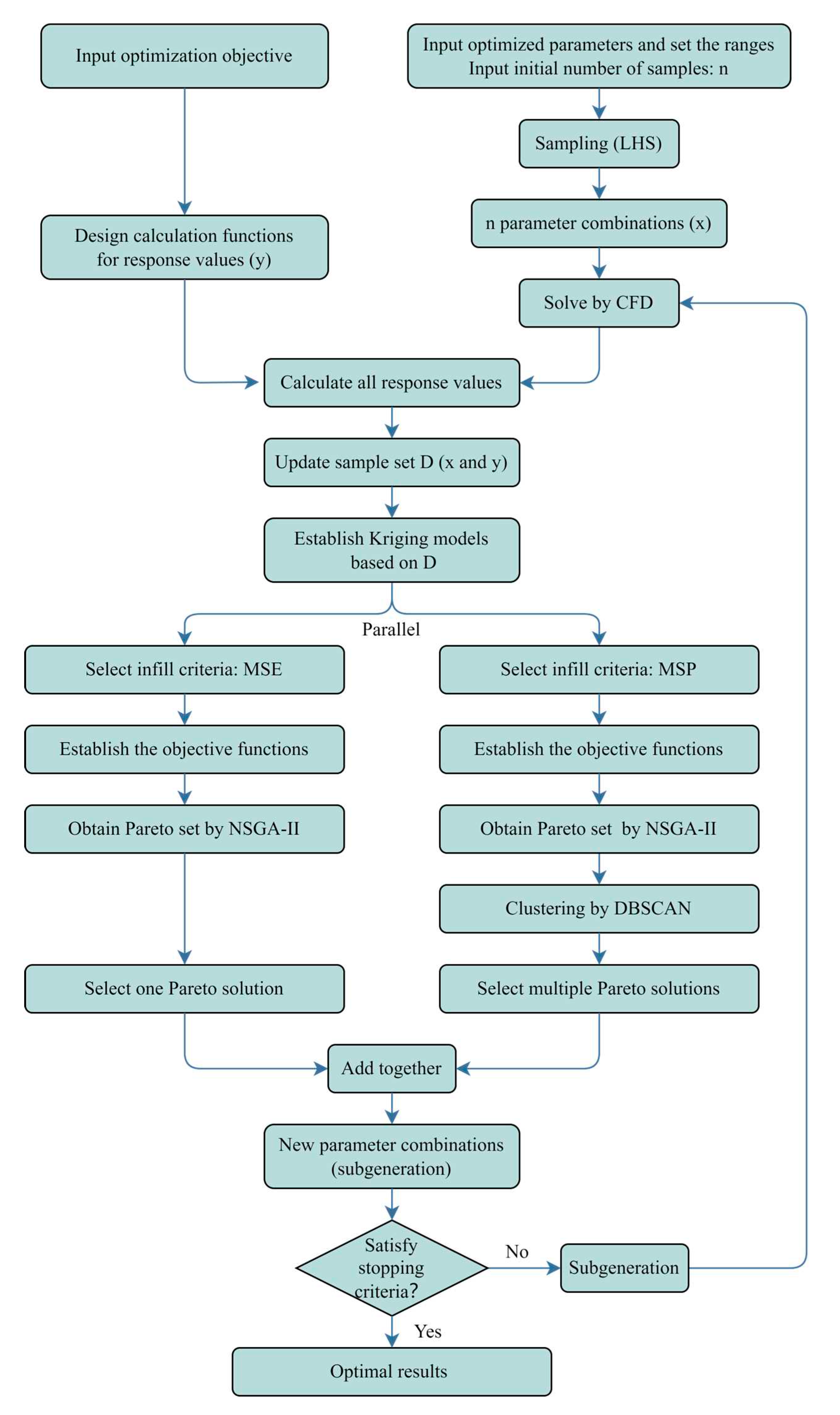
And ANN in Table 1 is mentioned again. In fact, not only ANN but also the other surrogate models mentioned above are widely used because creating an accurate surrogate model can effectively cope with the problem of long and costly CFD computation, which is of great importance in the field of real-time control. The methods using surrogate models have similar characteristics, while most of the recent studies use ANN, so the authors do not show other surrogate models separately in Table 1. But the major difference between surrogate-based methods and them is that it is not necessary to build an accurate enough surrogate model at the beginning of optimization, which will greatly reduce the number of samples. For example, Li, L. [17] used 3,356,496 samples to build the initial database. The approach when using surrogate-based optimization is to generate a number of parameter combinations, then calculate the target values (response values) and assemble them into an initial set (D) of samples. A surrogate model is built based on the set, a new combination of parameters (subgeneration) is generated by combining an infill criteria, the target values are calculated again and the set (D) is updated, and the process is repeated until global approximate optimal solutions are obtained [41]. Forrester, A. I. et al. [41] concluded that the initial parameter combinations were selected based on the space filling maximin [42] and the Latin hypercube sampling technique [43], which has excellent performance. In terms of infill criteria, there are minimizing surrogate model prediction (MSP) [44], mean squared error (MSE) [41], expected improvement [45], probability of improvement [46], etc.
Table 1 also shows that in the optimal design of air supply, there has been an increasing amount of study on multi-objective optimization in recent years compared to the previous single-objective optimization [2,3,4,47]. Because multi-objective optimization can provide designers with more options in some restricted scenarios. For example, by increasing the number of target areas, the Pareto set is obtained by multi-objective optimization to help us choose a more comprehensive air supply scheme.
Noteworthy is the POD method in the current study of air supply optimization, which, together with the surrogate-based methods, is based on an interpolation process and has a simplifying effect (at the expense of some accuracy) when dealing with super-many objectives (reconfiguration fields). With POD, the maximum number of interpolations does not exceed the minimum of the number of samples and the number of objectives (the rank of the matrix), so the number of interpolations can be reduced significantly by discarding some of the modes when dealing with super-multiple objectives. The POD method can also be applied to the surrogate-based optimization process to reduce the number of interpolations in the optimization of super-many objectives, and it will contribute to the development of agent-based super-many objectives optimization.
In general, meta-heuristic optimization approaches are too computationally expensive for multi-parameter air supply optimization, while gradient-based optimization is less computationally expensive but tends to fall into local optimum. Creating an accurate ANN is significant in the field of real-time control, but it is also costly for steady-state air supply optimization and equally costly to retrain the network in the event of errors. Surrogate-based optimization uses a surrogate model when generating subgeneration, which allows the subgeneration to be generated more efficiently in the right direction and reduces computational costs. However, there is a lack of research on this method in air supply optimization. Multi-objective optimization has advantages when dealing with antagonistic objectives. Evolutionary algorithms have been well proven to be very successful in finding well-converged and diverse non-dominated solutions in bi-objective optimization [48]. The Kriging model is a probabilistic surrogate model based on the Gaussian process and can be applied to a variety of infill criteria. Unlike dual-aisle cabins, dual-aisle cabins have a large span with occupants on both sides and in the middle, and therefore the thermal comfort requirements between them are likely to be antagonistic. In this paper, the authors first develop a double-objective optimization method based on NSGA-II [49] and the Kriging model and analyze its performance, then use the method to find the optimal design of a dual-aisle cabin for air supply (5 parameters) under dual-zone conditions.

2. Method Description

2.1. NSGA-II

NSGA is a dominance-based multi-objective optimization algorithm developed on genetic algorithms, where NSGA-II [50] overcomes some of the shortcomings of NSGA and has excellent performance in 2-3 objective optimization [48]. It can also be used for the optimization with more objective, although the overall results are worse than the NSGA-III performance [51]. Figure 1 is the flowchart:

2.2. Ordinary Kriging (OK) Model

The Kriging method is a full interpolation method. The approach can generate the most likely response value and variation at the projected location depending on the presumptions upon which it is based. The formula for its interpolation is Eq. (1), where c is the coefficient that needs to be solved for.
y ^ ( x ) = i = 1 n c i y x i
The subsequent deduction is then based on the assumption of the distribution of y. Eq. (2) is a common expression for the distribution:
y ( x ) = f ( x ) β + z ( x ) f ( x ) = ( f 1 ( x ) , , f n ' ( x ) )
where f(x) is the basis function (ordinary Kriging (OK) uses a basis function of 1 (zero polynomial); when f(x) is any other basis function, it is called universal Kriging), β is the coefficient, n' is the number of terms in the basis function, and z(x) is generally assumed to obey a normal distribution N(0, σ2). By minimizing the following expectations in Eq. (3), the interpolation process, which is a Gaussian process, gives the most likely response values and variances by solving the linear system of equations based on the Lagrange Multiplier Method.
min C o v ( ( y ( x ) y ^ ( x ) ) , ( y ( x ) y ^ ( x ) ) )
Its solution, which can be consulted through the literature [52], takes the following form as Eq. (4):
y ^ ( x ) = f ( x ) T β * + r T ( x ) γ * s 2 ( x ) = σ 2 ( 1 + u T ( F T R 1 F ) 1 u r T ( x ) R 1 r ( x ) ) β * = ( F T R 1 F ) 1 F T R 1 Y R γ * = Y F β * u = F T R 1 r ( x ) f ( x ) σ 2 = 1 m ( Y F β * ) T R 1 ( Y F β * ) r ( x ) = R ( x 1 , x ) , , R ( x n , x ) T R ( x ) = R ( x 1 , x 1 ) R ( x 1 , x n ) R ( x n , x 1 ) R ( x n , x n ) F = f ( x 1 ) , , f ( x n ) T Y = y ( x 1 ) , , y ( x n )
where x is the point that needs to be interpolated, xi (i = 1,...,n) is the known point, R(xi, xj) is the function that creates the correlation coefficients, R(x) is the matrix that only contains the correlation coefficients of the known points, and r(x) is the vector made up of the correlation coefficients of the point that needs to be interpolated and all of the known points. Based on the above, multiple OK models can be built from known data set and multiple objective functions can be developed. Then the NSGA-II method can be used to find the Pareto set.

2.3. Latin Hypercube Sampling

The initial sample set (D) is obtained by preparation, and this preparation is very important as it is a key factor in determining the error between the surrogate model and the actual function. If the surrogate model differs too much from the actual function, the process of continuously generating the next sampling points (subgeneration) through the surrogate model until it stops will become very long and may fall into a local optimum. Because of this, we want this sample set to cover as much of the globe as possible. As previously mentioned, current studies show that the Latin hypercube sampling (LHS) technique facilitates the generation of a high-quality initial sample set.
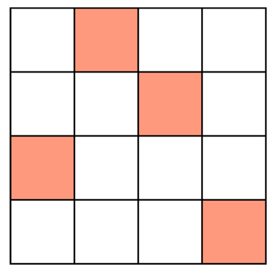
The Latin square (Figure 2) is a square (n × n) in which there are n different elements with one and only one element in the same row or column [53]. When expanding to m dimensions, all dimensions are first divided into n intervals with one and only one element in the same interval of each dimension, so that we only need n samples and their source includes all intervals for all parameters, unlike the grid-based sampling approach where the number of samples grows exponentially as the parameters increase.

2.4. Infill Criteria

A popular and successful strategy is to combine different infill criteria. In this study, MSE+MSP is utilized to increase the surrogate model's precision. This infill criteria has some ability to explore and exploit.
The MSE criteria takes the point at which the objective function is maximized as the new sampling object (the objective function consists of the variance (s2) of the probabilistic surrogate model), representing the exploration process, as in Eq. (5):
M a x F ( x ) = s 2 s . t . g ( x ) = 0
The MSP criteria takes the point at which the objective function is minimized as the new sampling object (the objective function is the predicted value of the surrogate model, which can be multiplied by -1 when the actual problem is to find the maximum value), representing the exploitation process, as in Eq. (6):
M i n F ( x ) = y ^ s . t . g ( x ) = 0
where g(x) is the constraint function, '→' refers to the vector.
In multi-objective optimization, the result usually exists as a Pareto set, and our goal is to obtain as true a Pareto Frontier as possible. Therefore, we need to select some Pareto solutions (points / new parameter combinations) to advance the Pareto Frontier in the right direction. It is worth noting that the points may form multiple clusters and that the shape of these clusters may be arbitrary. Filling according to clusters will significantly reduce the number of new samples.
The MSE criteria and the MSP criteria play different roles in the optimization process, as the MSP criteria will usually provide the results we want. Therefore, in this paper, when constructing the objective functions for multi-objective optimization using the MSE criteria, a Pareto solution is selected from the Pareto set, and the point is used as the new sampling object. When constructing the objective functions for multi-objective optimization using the MSP criteria, the set X of points corresponding to the Pareto set is first clustered, and then some points (with the smallest weighting value) in partial clusters are selected as the next sampling points to contain more information in fewer samples and to quickly approach the true Pareto Frontier. In this paper, Density-Based Spatial Clustering of Applications with Noise (DBSCAN) [54] is used in order to discover clusters with arbitrary shapes. The parameters necessary for the algorithm are the neighborhood radius (d) and the minimum number of points (p) within the radius. The process of the algorithm is as follows:
  • All objects (points) in the initial set X are marked as 'unvisited';
  • Select an unvisited object x randomly, mark x as 'visited', and check whether the neighborhood of x contains at least p objects;
  • If not, then x is marked as a noise point. Otherwise, a new cluster C is created for x, and all objects in the neighborhood of x are placed in the candidate set N;
  • Add objects that do not belong to other clusters from N to C iteratively. In this process, for an object u from N marked as 'unvisited', mark it as 'visited' and check its neighborhood, and if the neighborhood of u contains at least p objects, then all objects in the neighbourhood of u are added to N. Continue adding objects to C until C cannot be extended (N is empty). Then the generation of cluster C is complete;
  • Select an unvisited object at random from the remaining objects and repeat steps 2 and 3 until all objects have been visited.
As the units of the parameters being optimized are usually different, this paper clusters by performing a dimensionless operation and maps the parameters to an interval with width 1.

2.5. Process of Optimization

The optimization process in this paper is shown in Figure 3.
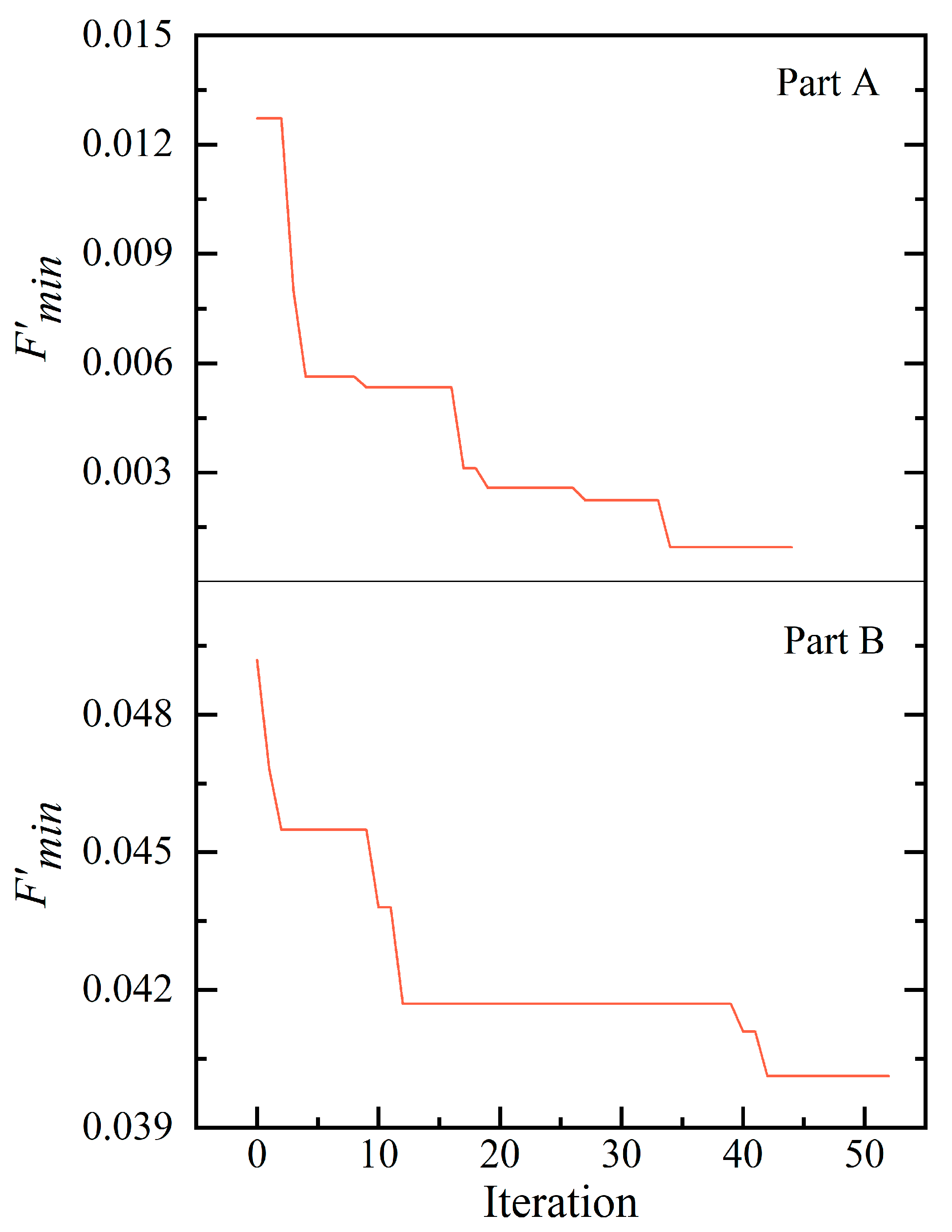
The stopping criteria used in this paper is that the minimum value F'min of the weighted sum F' with respect to the two objective functions F1 and F2 in all solved samples, remains unchanged after s (in this paper, s = 10) iterations.

3. Testing with a Simple Room Case

Inverse prediction of boundary conditions by some data (simulation-based or experiment-based) to test the optimization capability of the method. Since the optimal result is known for the inverse prediction, this test is convenient and effective.

3.1. Descriptions of the Case

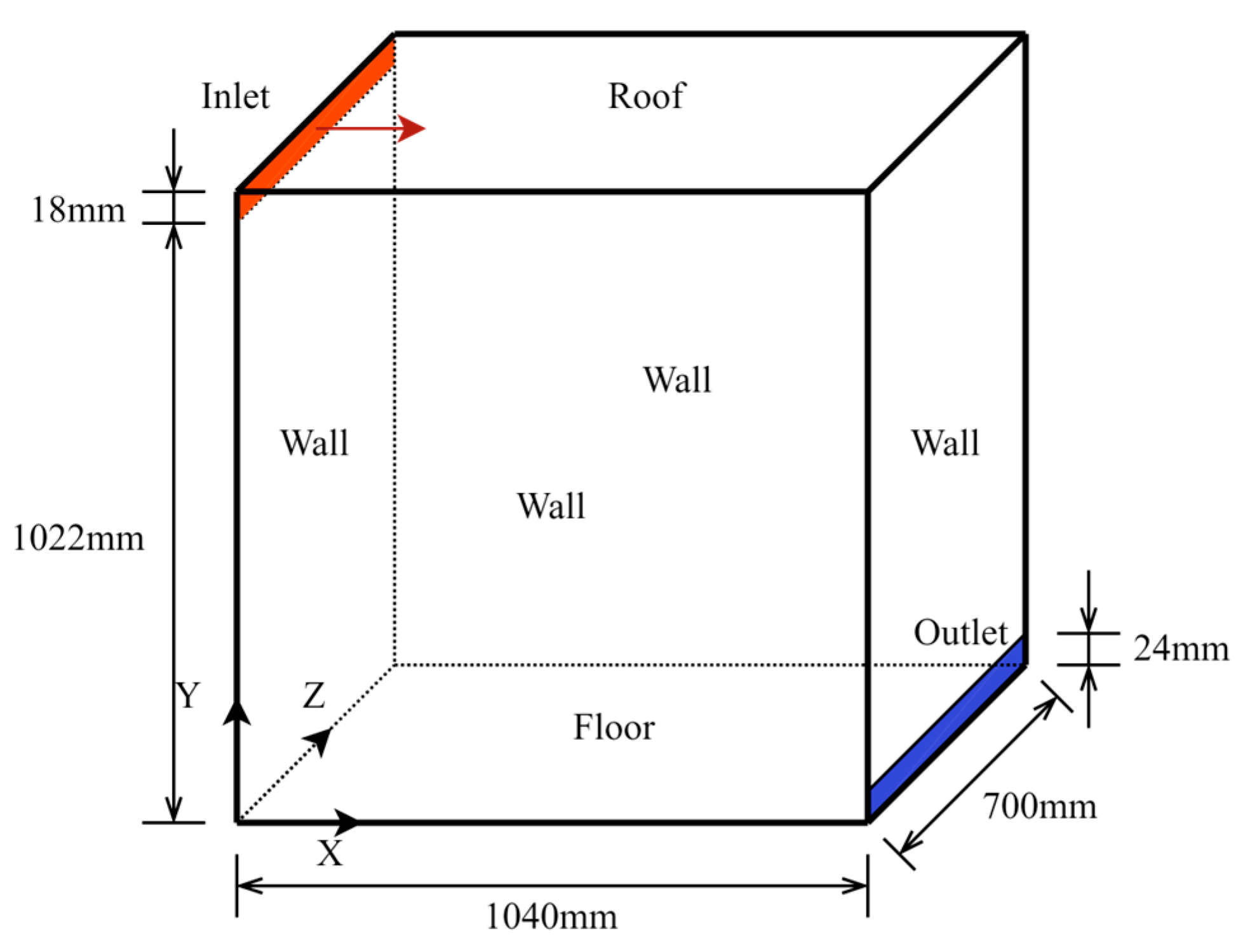
A non-isothermal convection case [55], which provides experimental data on air velocity and temperature at some locations under several boundary conditions was used. Xue, Y [4] also used this case to conduct a test of the CFD-based genetic algorithm method. And Figure 4 illustrates the case. The temperature (Tin) and velocity (Vin) of the inlet air are 15 ℃ and 0.57 m/s, respectively; the temperature of the roof (Troof) and the wall (Twall) are equal to Tin, and the temperature of the floor (Tfloor) is 35.5 ℃. Tin and Vin are the targets for the inverse prediction, so they were used as the optimized parameters.

3.2. Test Method

Inverse prediction tests are carried out using Computational Fluid Dynamics (CFD) simulations. Inverse prediction is similar to finding the inverse function in that there may be multiple solutions for a single target value. Although we have experimentally obtained data for some physical quantities under a certain boundary condition, we may obtain multiple boundary conditions by making inverse predictions based on some of the data. Using more data reduces the likelihood of multiple solutions, and when there is enough data, the solution should be unique. Because we know that these data are obtained from our forward-based experiments and we believe that our simulations are accurate. Xue, Y [4] used velocity and temperature data from all locations and his test method was:
  • Construct the objective/cost function as in Eq. (7) (minimization, which can be seen as a "distance");
    F = 1 3 ( u ^ y u y ) 2 u y 2 + ( u ^ x u x ) 2 u x 2 + ( t ^ t ) 2 t 2
  • Set parameter range: 0 < Vin < 1 m/s, 0 < Tin < 20 ℃;
  • Minimize the objective function by a single-objective genetic algorithm and output the corresponding parameters.
In fact, Xue, Y considered all physical quantities have the same weight after the same dimensionless process when performing step 1). It was also a process of converting from multiple-objective to single-objective. Since experiments are subject to errors and different CFD models differ in their solution results, especially in the near-wall region [56], it is difficult to obtain exactly the same results as experiments in simulations. It leads to the possibility that there is no one combination of parameters that makes the simulation results identical to the experimental results, so that the optimization algorithm can only obtain a set of parameter combinations (possibly not identical to the parameters used in the experiments) that make the simulation results "closest" to the experimental results at the defined "distance" (objective function). Xue, Y encountered this problem when making inverse predictions based on experimental data. In this paper, the physical quantities are separated to form an objective function with respect to uy and an objective function with respect to t. The following conditions are required to use NSGA-II. Where D is a sample set consisting of some parameter combinations and their response values obtained based on the simulation results and calculation functions.
  • Construct the objective function as in Eq. (8). Using MSP criteria as an example;
F 1 = y ^ | O K u y ( D ) F 2 = y ^ | O K t ( D )
where OKuy(D) and OKt(D) are OK models obtained by interpolating from D. Their response values yn at known points xn are calculated as Eq. (9):
O K u y ( D ) : y n ' = i = 2 9 u ^ ¯ y i n u y i 1 y n = y n ' max ( y n ' ) O K t ( D ) : y n ' = j = 3 9 t ^ ¯ j n 273.15 t j 273.15 1 y n = y n ' max ( y n ' )
where n represents the nth known point (parameter combination), i, j correspond to the order in the data sheet in Appendixes A and B, and '—' indicates averaging.
2.
Set parameter range: 0 < Vin < 1 m/s, 0 < Tin <20 ℃.
In this paper, it is considered that the direction that can minimize both objective functions (representing the simultaneous use of velocity and temperature data for inverse prediction) is more important in this case, so F1 and F2 are both weighted at 0.5. Then the inverse prediction is carried out according to an optimization process of Section 2.5. The initial samples size were 20.

3.3. Inverse Prediction Results

The inverse prediction was first based on the simulation data obtained through 2D simulation under experimental boundary condition (Tin and Vin of the inlet air are 15 ℃ and 0.57 m/s) to quickly explore the performance of the method in this paper (Xue, Y was unable to obtain very accurate results when making inverse predictions based on experimental data, so he again made inverse predictions based on simulation data to demonstrate the optimization capability of the CFD-based genetic algorithm). Then 3D simulations were used based on experimental data to explore problems that may be encountered in practical applications of the method (The air supply scenarios that can be translated into 2D are relatively few). Figure 5 shows the change curve about F'min for the two scenarios (Part A:Based on simulation data and 2D simulations; Part B:Based on experimental data and 3D simulations), where Part B had made some other additions to the optimization process, which will be described in detail in Section 3.3.2.

3.3.1. Based on Simulation Data and 2D Simulations

Based on the simulation data using 2D simulations for inverse prediction, the output Pareto set is shown in Table 2:
As an inverse prediction based on simulation data, the true Pareto set should be a single point (Xue,Y obtained unbiased results when using the genetic algorithm and simulation data in his inverse prediction), and the above results indicate that the method can only provide approximate results. One reason is that the objective functions established from the velocity and temperature data at the above positions are all very small in some directions. In the vicinity of the correct boundary condition, smaller Vin leads to an increase in temperature, and smaller Tin leads to an increase in the buoyancy force (increasing the velocity, especially in the Y-direction), resulting in very small values of F1 or F2 in a direction. This direction is different for F1 and F2, so it is easy to produce non-dominated solutions when sampling near the correct boundary condition.
In addition, because of the errors of the OK models and the use of continuous populations (continuous optimization) when using NSGA-II, it was difficult to select the correct parameter combination directly. However, the current Pareto Frontier is close enough to the true Pareto Frontier. When using the boundary condition corresponding to F'min as the final result (representing the simultaneous use of velocity and temperature data for inverse prediction), result 1 in Table 2 is already very close to the correct boundary condition.

3.3.2. Based on Experimental Data and 3D Simulations

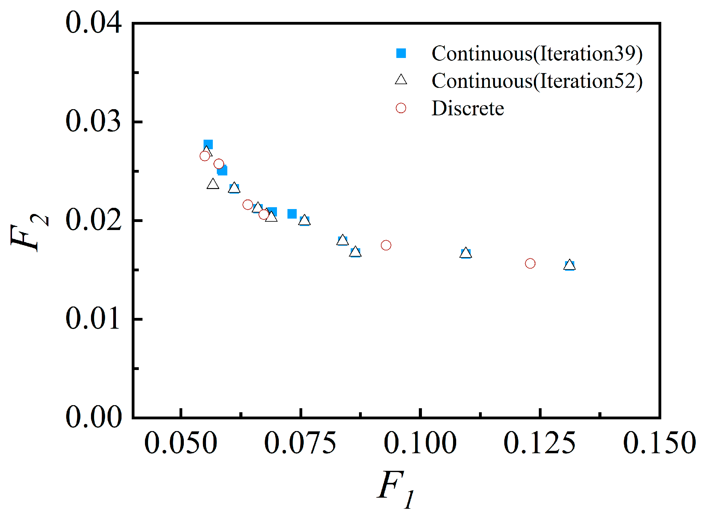
The inverse predictions are based on experimental data and 3D simulations. Some of the particular non-dominated solutions generated in NSGA-II using continuous populations (continuous optimization) or discrete populations (discrete optimization) are shown in Table 3. Figure 6 shows the Pareto Frontiers.
Because of the differences between experiments and simulations, inverse predictions based on experimental data are more likely to be biased. According to the stopping criteria (Within s consecutive iteration steps, F'min remains constant) in Section 2.5, the optimization should have been stopped before Iteration 39, but the optimization was continued because the inverse prediction was not satisfactory (The deviation of the solution corresponding to F'min is still large). In order to determine if a better outcome might be reached, a bigger s was used. However, it was shown to be difficult for this case. The authors analyze some reasons for this, using F1 as an example:
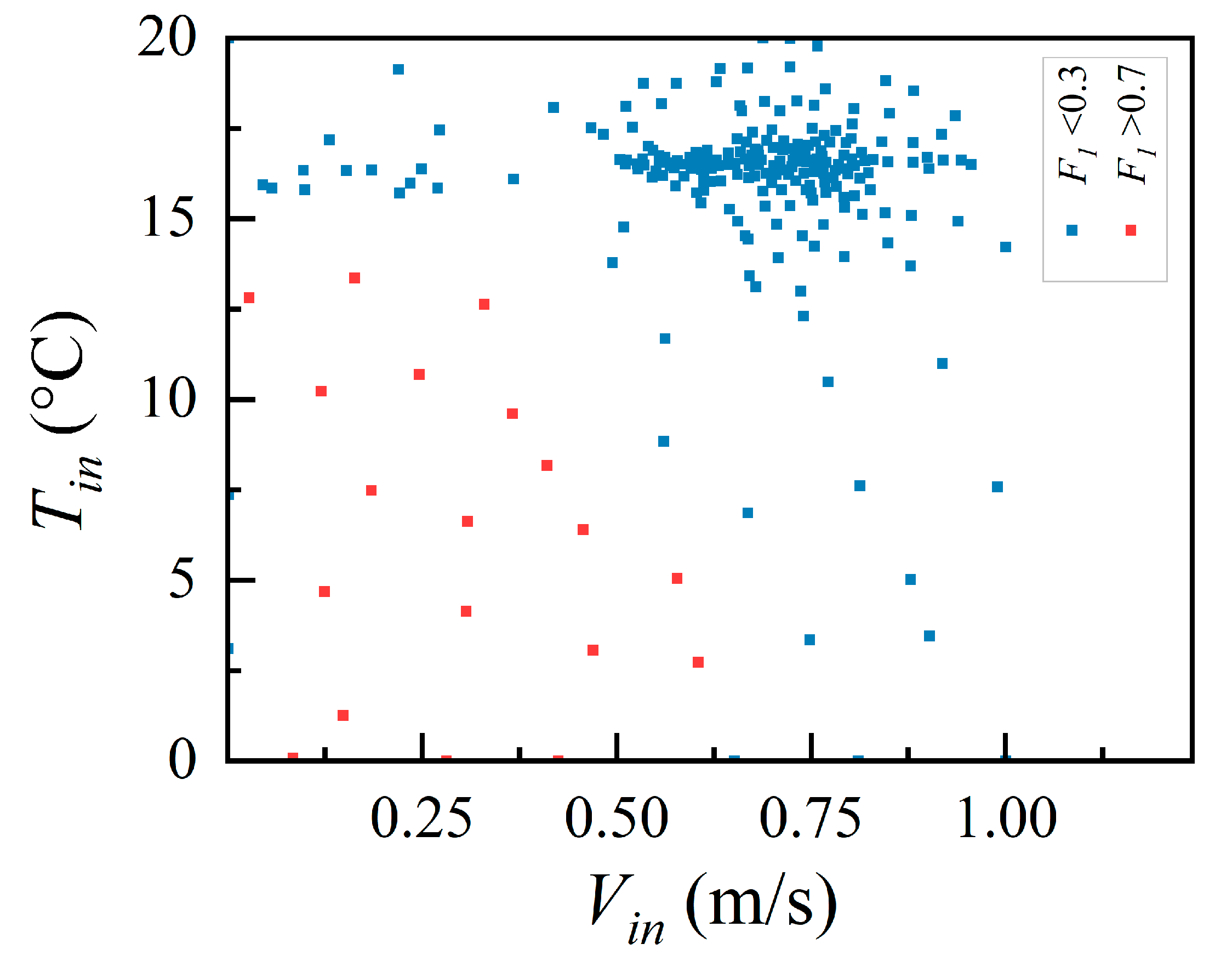
Figure 7 shows the presence of a sudden change in F1 (Samples with red label: F1 > 0.7); samples with blue label: F1 < 0.3), corresponding to the inversion of the flow field in this case [55]. This also reveals that there are some abrupt changes in the air delivery optimization, contrary to most of the optimizations performed based on the continuity assumption. As the Kriging method is also a smooth interpolation method, this dictates that the method may does not handle this problem well. But this problem is not the most important (According to section 3.3.1, when facing this problem, the results obtained from inverse prediction based on 2D simulation are still accurate). A more critical problem is that the results of 3D steady-state simulations are usually unstable; any physical quantity at any position usually fluctuates and does not converge to a stable value as in a 2D steady-state simulation. As Figure 8 shows, although 2000 iteration steps were used to average the velocity values for each location, F1 still had rapid and irregular changes in some areas. The large gradient caused the OK models to believe that the minimum value would be generated in these areas. So the filling process always took place in these areas. For this 3D inverse prediction, from Iteration 20 to Iteration 39, most of the new samples were in the area shown in Figure 8. Therefore, from Iteration 40, the parameter range was adjusted to: 0.4 < Vin < 0.7 m/s, 10 <Tin < 20 ℃.
In other words, the problem expressed above is that the results of 3D steady-state simulations are usually unstable, so that the response values have both 'global' and 'local' variation. And the 'local' variation can be rapid in some areas, which can seriously affect the accuracy of the OK model and influence the generation of subgeneration in the right direction.
For the previous inverse predictions, the populations used in NSGA-II are continuous. If an acceptable precision is provided for each parameter and the precision is much smaller than the scale required for 'global' variation and larger than the scale required for 'local' variation, it is beneficial to filter the tiny structure in the OK models and reduce the possibility of oversized gradients occurring when using a discrete population search surrogate model and generating new sampling points (subgeneration). It may lead to faster optimization and equally accurate results. For realistic air supply processes, the control accuracy is also limited, so such a choice is usually acceptable.
Set the precision of Vin to 0.01 m/s and the precision of Tin to 0.1 ℃ without shortening the interval, and restart the optimization using the same initial samples. The number of iterations at the end of the optimization is 12, and part of Pareto solutions are as in Table 3.
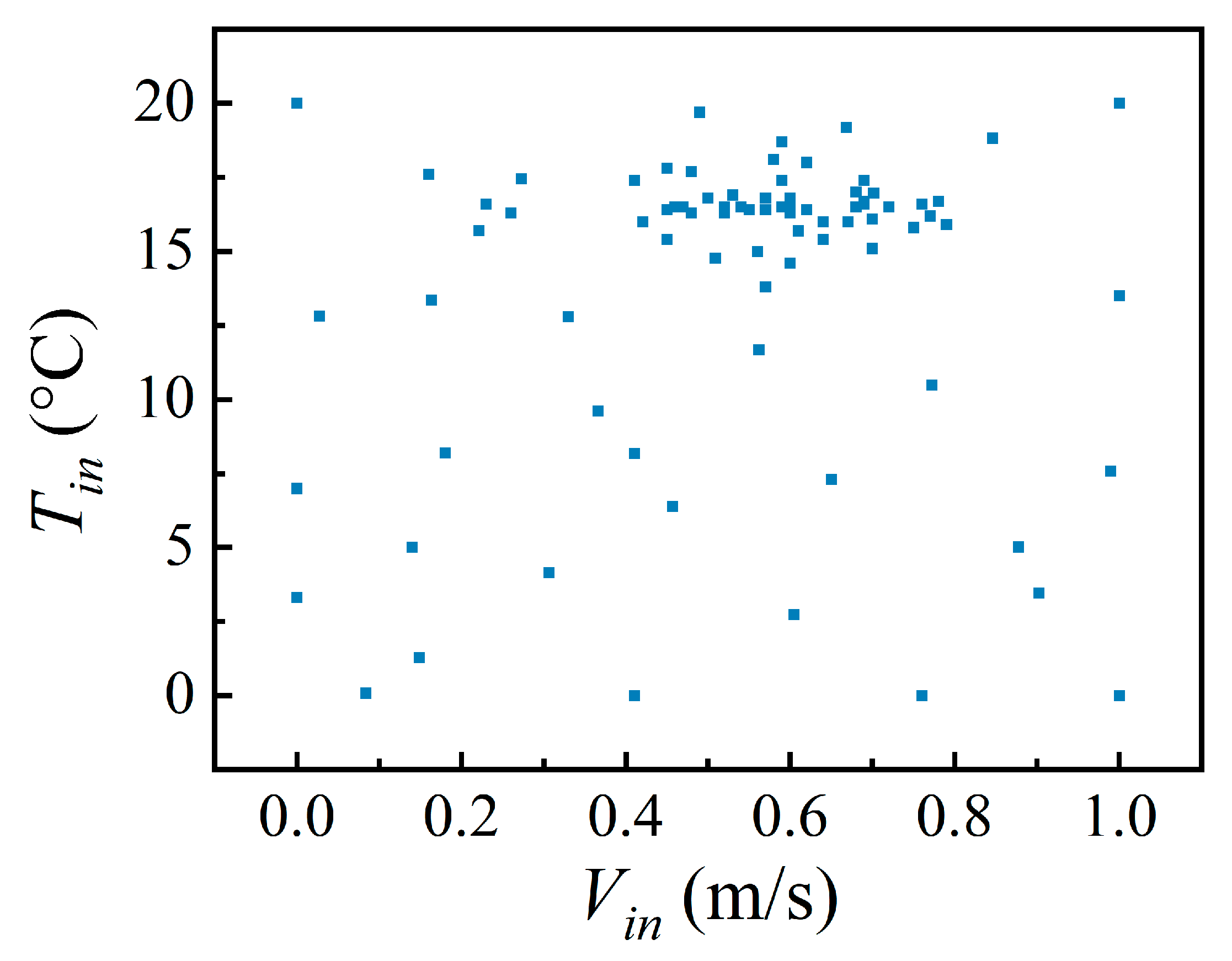
It can be seen that for inverse predictions based on 3D steady-state simulations, the use of discrete populations has little effect on the accuracy of the inverse prediction results compared to the use of continuous populations because of the presence of 'overall' variation and the use of a small discrete length. They produced very close Pareto Frontiers (Figure 6). Figure 7 and Figure 9 show that the number of samples became smaller in the area mentioned in Figure 8 compared to the other areas, and the total number of samples has also decreased.
From the above study, for this case, the method in this paper can quickly achieve an approximate prediction of the inlet boundary condition, and the non-dominated solutions provided can be considered as inverse prediction results for different weight combinations of velocity and temperature data. Unlike genetic algorithms that directly use selection operator, crossover operator and mutation operator to generate a subgeneration with many individuals and maintain diversity, the method in this paper uses OK surrogate model built on the assumption of continuity and smoothness to generate a subgeneration with few individuals and uses the MSE criteria to maintain diversity. It significantly reduces the number of individuals in subgenerations, improves sample utilization and maintains the global search capability. However, the OK model's error reduces the likelihood that the subgeneration appear in the right direction in cases where the response values change quickly, are locally non-differentiable, or are intermittent. And the results may not be as accurate as the genetic algorithm.

4. Optimizing the Air Supply Parameters of a Dual-Aisle Single-Row Cabin

4.1. Case Descriptions

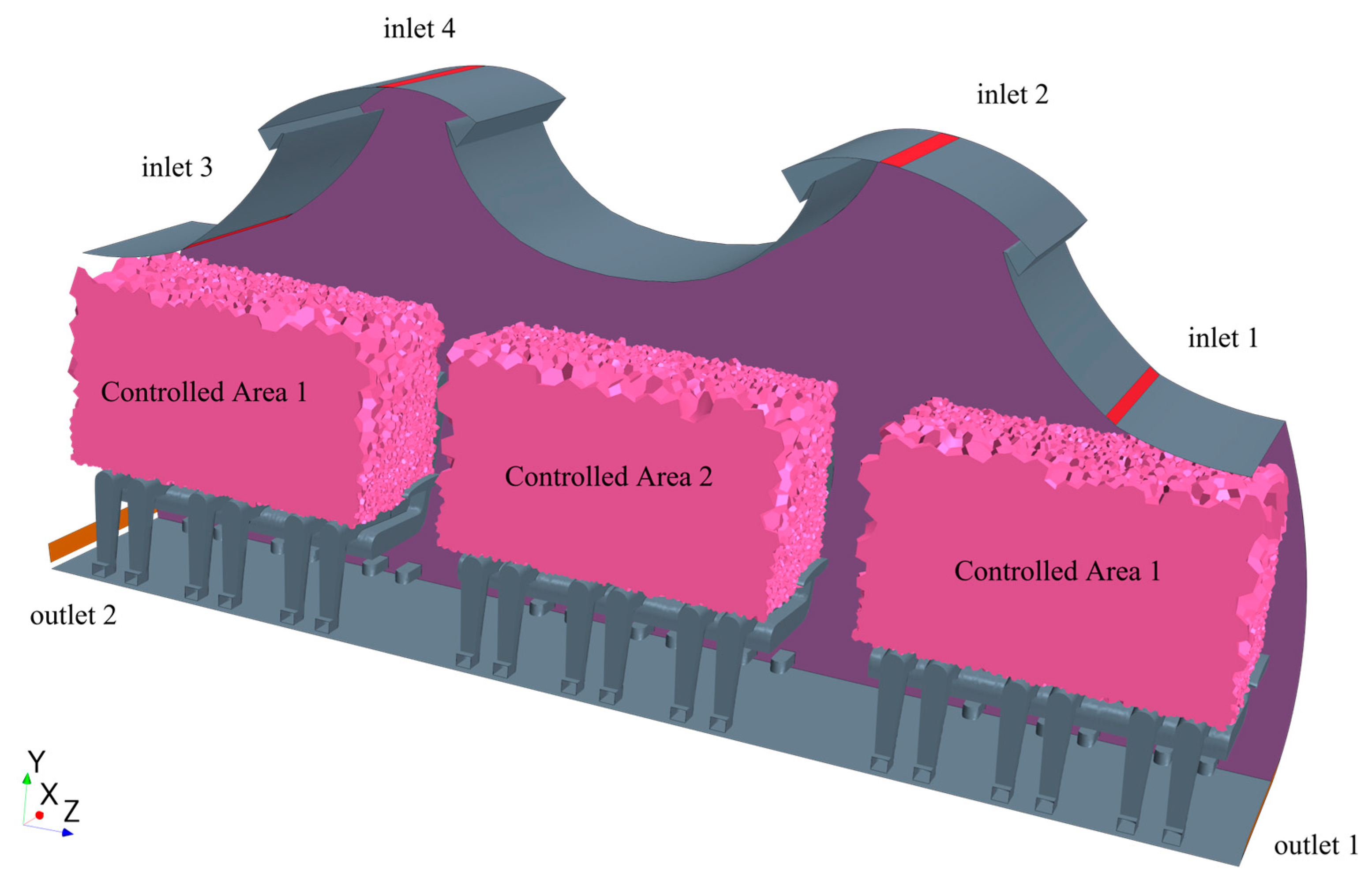
As described in Figure 10, the cabin had four air inlets, the wall temperatures on both sides were set to 21 ℃ [4], the upper and lower surfaces were set to adiabatic, and the front and rear cross sections were set to interface. Referring to the setting of Yang (2016) [57], the human body surface temperature in this case was divided into three levels (head: 28.65 ℃, body: 32.1 ℃, legs: 33.07 ℃). The objective of the optimization was to create a comfortable thermal environment for the upper body areas of all occupants. Based on the analysis of the airflow organization (mainstream converged in the middle) in single-aisle cabin optimization results [47], the two-aisle cabin was likely to face the problem that directly using a total volume satisfying |PMV| (Predicted Mean Vote) < 0.5 as a single objective might neglect local thermal comfort (discarding middle or side occupants). Therefore, it was divided into two controlled areas in this paper (the volumes of controlled areas 1 and 2 are 1.47 and 0.73 m3 respectively). In addition, for this symmetrical structure, it is common practice to use a symmetrical air supply or to use a half cabin for the simulation, which is commonly used in the cabin air supply and optimization processes. This also reduces the number of parameters to make optimization less difficult, so the same symmetric air supply approach was used in this paper. In accordance with the optimization objective, the response values of the samples yn used to build the OK models were defined by Eq. (10):
O K v o l u m e 1 ( D ) : y n ' = a v e r a g e ( V = Controlled   Area   1 I F ( P M V < 0.5 ) d V ) y n = y n ' max ( y n ' ) O K v o l u m e 2 ( D ) : y n ' = a v e r a g e ( V = Controlled   Area   2 I F ( P M V < 0.5 ) d V ) y n = y n ' max ( y n ' )
where V refers to the integrated region (the controlled areas), PMV refers to the PMV value of dV, the averaging function is used for averaging, and the IF function returns 1 when its internal expression is satisfied; otherwise, it returns 0.
The objective function is defined as Eq. (11) (MSP side):
F 1 = y ^ | O K v o l u m e 1 ( D ) F 2 = y ^ | O K v o l u m e 2 ( D )
Maximizing the total volume is also a primary interest in this paper, so the weights are taken as 0.67 for F1 and 0.33 for F2. Because of the more parameters, the initial sample size is changed to 60. Otherwise, the optimization tends to fall into a local optimum, which is similar to meta-heuristic optimization approaches.
According to the viewpoint of Figure 10, with X as the axis of rotation and the direction of the air supply outlet normal vector as the starting direction, the counterclockwise rotation is positive and the range of the air supply outlet angle (θ) is all limited to -80 °< θ < 80 °. During normal operation of the aircraft's air conditioning system, it should be ensured that the amount of air supplied to each occupant is greater than 0.25 kg/min [58], so the upper and lower limits of air velocity (V) are 0.1 m/s and 1.5 m/s. The upper and lower limits of temperature (t) are 8 ℃ and 20 ℃. Therefore, the number of air supply parameters to be optimized is 5 (t, V1, V2, θ1, θ2), subscripts 1 and 2 refer to the numbers of the air inlets in Figure 10. The parameters' range and their accuracy are listed in Table 4:

4.2. Optimization Results

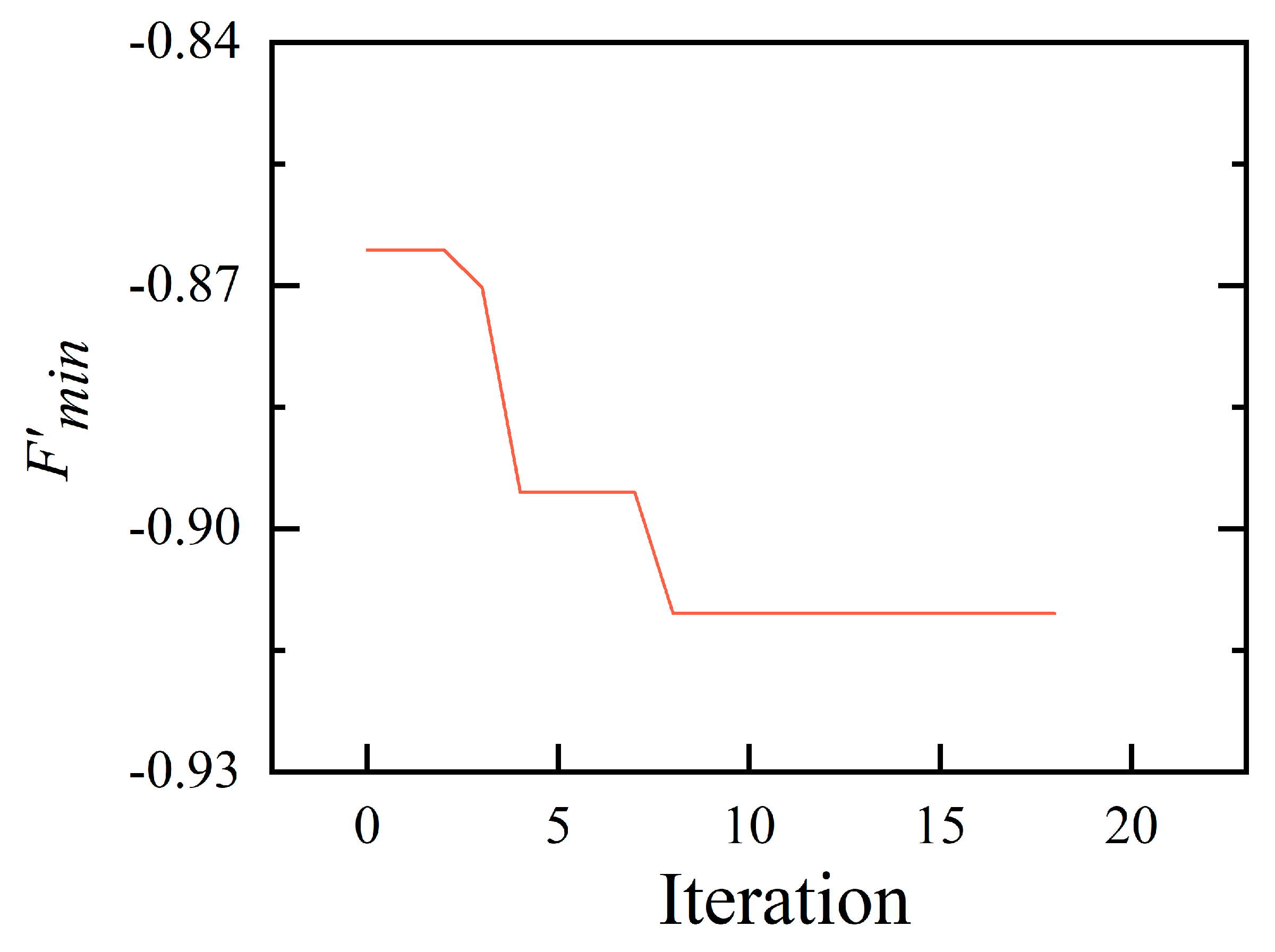
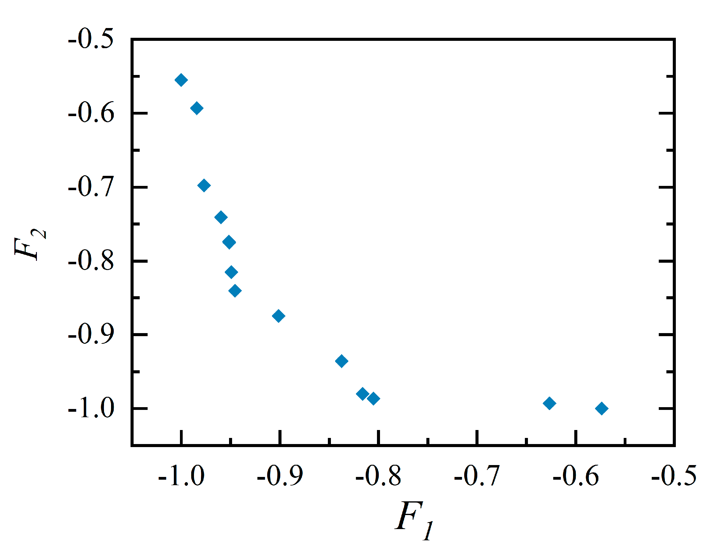
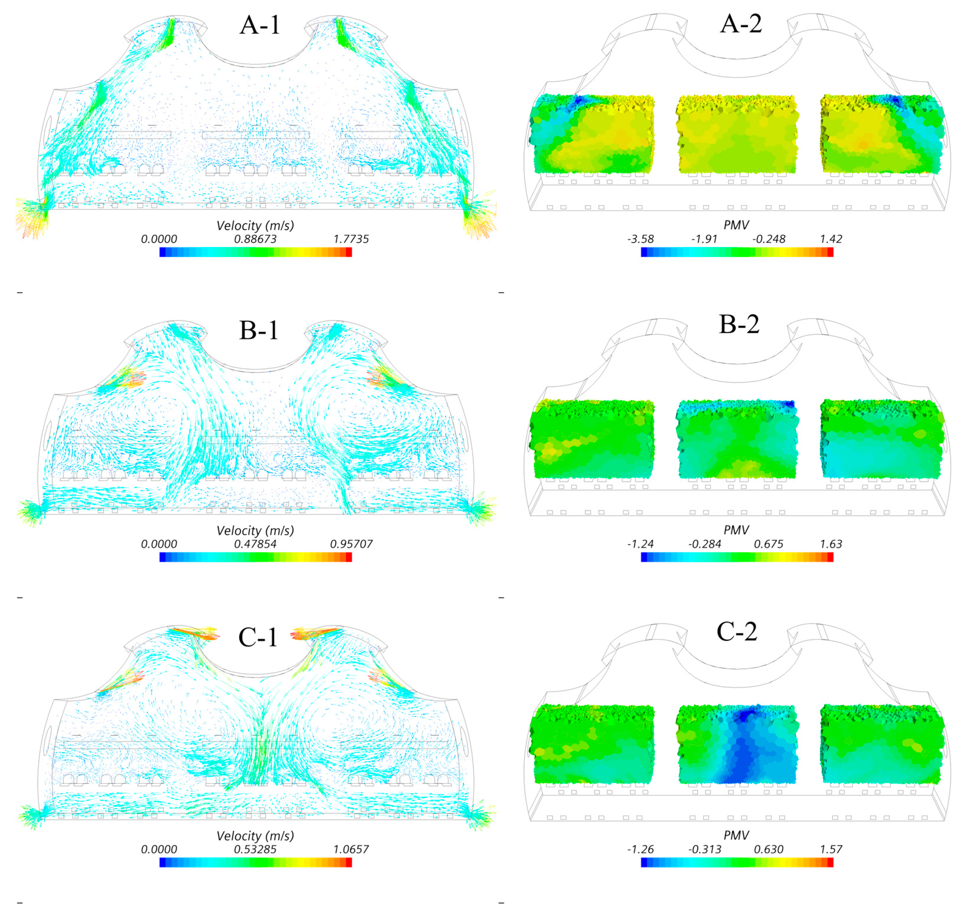
Figure 11 shows the change in F'min, where the abrupt drop in Iteration 4 was caused by a switch from an A-shaped to a B-shaped airflow organization (Figure 13). And after Iteration 8, some non-dominated solutions were obtained, but F'min did not decrease. While Figure 12 shows the Pareto Frontier with all non-dominated solutions. For such a 5-parameter optimization process, a fully meta-heuristic optimization approach may require thousands of samples to obtain a reliable optimization result.
Table 5 shows information on some of the non-dominated solutions. Solutions 1, 3, and 9 correspond to A, B, and C in Figure 13, respectively.
The above results show that the thermal comfort of the occupants in the two zones is antagonistic and cannot be maximized at the same time because of the limitations of the air supply. Case A shows the form of airflow organization that is present when maximizing the thermal comfort of the middle occupants, and it can be seen that the thermal comfort of the occupants on both sides is completely abandoned, while the opposite is true for case C. Case B is probably the best, as the airflow on each side converges from the aisle to the bottom, creating two symmetrical loops, with only the middle occupant near the aisle being slightly affected by the cold air. The other Pareto solutions (Figure 12) correspond to less favourable situations.
Furthermore, the concave Pareto Frontier makes the total volume be maximized in case B (located in the middle part of the Pareto Frontier). So there is no need to completely abandon a region to obtain the maximum total volume, which should be consistent with the optimal solution obtained by single-objective optimization using the total volume.
According to additional study of the non-dominated solutions surrounding solution 3 through Table 5, the air supply parameters (solutions 2-8) show small variation. It shows that the requirements for forming the airflow organization depicted in B in the two-aisle cabin are more demanding and that the effect of raising supply air temperature on the PMV cannot be mitigated by raising air velocity [4] as in the single-aisle cabin, where there is no occupant in the middle.
For example, once the air velocity at the bottom air inlets has been increased, the airflow cannot form a rounded airflow like B at low angles of air supply, and the airflow will be directed towards the occupants next to the aisle, while at high angles of air supply, an airflow organization similar to that shown in C will form, meaning that the thermal comfort of the occupants in the middle is sacrificed. For the case of decreasing the temperature and velocity and increasing the angle, there is a lack of samples, as the surrogate model may again show large errors in the face of such scenarios with rapidly changing response values. The subgeneration are not generated in this direction, and the optimization seems to have stalled, so the method still needs to be refined. However, it can be assumed that the 'length' of this direction will not be too long, as the high angle and low air velocity mean that the air supply drops off quickly and the upper air inlets will take on more of the air supply load and dominate the airflow in the cabin. The authors conducted their analysis by examining samples that would create an airflow organization like A or C if the upper air inlets had a higher air velocity.

5. Discussions

In this study, a surrogate-based double-objective optimization method is developed, and some non-dominated solutions are obtained by a small number of simulations in an air supply scenario with 5 parameters. The results are similar to those in other studies in terms of cost, which provides a new option for air supply system designers. However, this method can only provide approximate optimal solutions because the surrogate model based on the results of 3D steady-state simulation is prone to errors.
Some of the current problems with optimization methods based on continuous, smooth-type surrogate models are that they do not adapt well to scenarios where the response values change quickly, are locally non-differentiable, or are intermittent. Sometimes optimization can stall as a result, essentially because the model generates large gradients and errors, and the subgeneration (new parameter combinations) become less likely to be generated in the correct direction. Using surrogate models with gradient information may alleviate this problem.
By analyzing some studies of CFD-based genetic algorithms [4,10,26,28,29,59,60] and POD methods[5,6,24,25,61], viewing the source code (such as Geatpy), and communicating with some of the authors, a summary of the three methods (including the method of this paper) was made, as shown in Table 6. Of course, the table analyzed only the simplest form of each method and did not include various types of variants, such as the co-evolution of multiple populations in genetic algorithms. Where the gradient dependence comes from the continuity assumption and the interpolation method.
Secondly, infill criteria need further study because one of the main objectives of this study is to reduce the computational cost. Therefore, the Pareto set is processed using a clustering algorithm, which is likely to overlook the more significant non-dominated solutions since it uses a small number of solutions to represent the current Pareto set. During the optimization in Section 4, we also found that when facing high-dimensional scenarios (multi-parameter), the subgeneration provided by the MSE side significantly lag behind the MSP side in terms of exploration speed (diversity), and a reasonable ratio needs to be designed for them.

6. Conclusions

The above study and the analysis of the results lead to the following conclusions:
  • In some common scenarios, the method in this paper can quickly provide an approximate Pareto Frontier. However, in the face of scenarios where the response values change rapidly, are locally non-differentiable, or are intermittent (surrogate models generate large gradients, and model errors make it challenging to optimize correctly), the optimization may stall. Because this paper assumes that the response values should be continuous and smooth, and then the Kriging model is used. Therefore, the method is more suitable for scenarios where the response values vary gently. In optimization based on 3D steady-state simulation, the use of discrete optimization with an appropriate discrete length can alleviate the above problems, speed up the optimization, and maintain accuracy.
  • The method in this paper, as a development of meta-heuristic optimization approaches, also has global search capability when a sufficient number of initial samples are provided. The difference is that the method generates a subgeneration with few individuals based on the prediction of the surrogate model, which improves the utilization of the samples, makes the subgeneration more likely to be generated in the right direction, greatly reduces the total number of samples, and reduces the computational cost. However, compared with the meta-heuristic optimization approaches that use selection operator, crossover operator and mutation operator to generate a subgeneration with many individuals directly, the diversity of subgeneration and the adaptability of method decrease.
  • After dividing the dual-aisle cabin into two zones, the air supply parameters were optimized using this paper's method. 118 samples (cases) were calculated to obtain an approximate Pareto Frontier. For such a 5-parameter optimization process, thousands of samples may be required based on meta-heuristic optimization approaches. When using the POD method, if each parameter is divided into 4 intervals, uniform sampling requires 3125 cases to compose the initial database. The generated Pareto set suggests that an airflow organization with a left-right symmetric circulation structure may be optimal.

Author Contributions

Yu Guo: Writing – review & editing, Writing – original draft, Visualization, Validation, Software, Resources, Project administration, Methodology, Investigation, Formal analysis, Data curation, Conceptualization. Yukun Wang: Writing – review & editing, Validation, Methodology, Investigation, Data curation, Conceptualization. Yi Cao: Validation, Supervision, Resources, Project administration, Investigation, Funding acquisition. Zhengwei Long: Writing – review & editing, Validation, Supervision, Project administration, Methodology, Funding acquisition, Conceptualization.

Funding

The research presented in this paper was supported by National Nature Science Foundation of China (Grant No.51878442).

Data Availability Statement

Data will be made available on request.

Conflicts of Interest

The authors declare that they have no known competing financial interests or personal relationships that could have appeared to influence the work reported in this paper.

Nomenclature

c Coefficient of OK model (-) y(x) The distribution of predicted value
C Cluster (-) z(x) Error function of the Kriging model
d Neighborhood radius (-)
D Sample set (-) Superscripts/Subscripts
m Dimensionality (-) - Average
n Initial sample size (-) ^ Predicted value
N Candidate set in clustering (-) 1 / 2 A number
p Minimum number of points in clustering (-) i / j A number
s Number of iteration steps (-) in Inlet
T Temperature (℃) n A number
u Object in clustering (-)
V Velocity (m/s) Greek symbols
x Variable (-) σ Standard deviation (-)
X Initial set in clustering (-) θ Angle (°)
Functions Abbreviations
average(x) Average function ANN Artificial neural networks
Cov(xi,xj) Covariance function LHS Latin hypercube sampling
f(x) Basis function of the Kriging model MSE Mean squared error
F(x) Objective (cost) function MSP Minimizing surrogate model prediction
F'(x) Combinatorial function of the objective function NSGA Non-dominated Sorting Genetic Algorithms
g(x) Constraint function OK Ordinary Kriging model
IF Logic function PMV Predicted Mean Vote
max(x) Find the maximum POD Proper orthogonal decomposition
R(xi,xj) Function of correlation coefficient PSO Particle swarm optimization

Appendix A

Part of the experimental data (uyi)
y=0.52m, z=0.35m
i 1 2 3 4 5 6 7 8 9 10
xi (m) 0.024 0.063 0.102 0.205 0.354 0.709 0.859 0.961 0.985 1.020
uyi (m/s) 0.220 0.240 0.222 0.140 0.068 -0.06 -0.125 -0.204 -0.268 -0.270
Notes: Data from Blay's experimental study [55].

Appendix B

Part of the experimental data (tj)
y=0.52m, z=0.35m
j 1 2 3 4 5 6 7 8 9 10 11
xj (m) 0.00 0.02 0.038 0.084 0.229 0.520 0.811 0.964 1.00 1.01 1.04
tj (K) 288 292 293 293 292 292 292 291 291 291 288
Notes: Data from Blay's experimental study [55].

References

  1. Pironneau, O. (1974). On optimum design in fluid mechanics. Journal of fluid mechanics, 64(1), 97-110. [CrossRef]
  2. Liu, W., & Chen, Q. (2015). Optimal air distribution design in enclosed spaces using an adjoint method. Inverse Problems in Science and Engineering, 23(5), 760-779. [CrossRef]
  3. Malkawi, A. M., Srinivasan, R. S., Yi, Y. K., & Choudhary, R. (2003). Performance-based design evolution: The use of genetic algorithms and CFD. Eighth International IBPSA. Eindhoven, Netherlands, 793-798.
  4. Xue, Y., Zhai, Z. J., & Chen, Q. (2013). Inverse prediction and optimization of flow control conditions for confined spaces using a CFD-based genetic algorithm. Building and Environment,64, 77-84. [CrossRef]
  5. Wang, J., Zhou, H., Zhang, T., & Wang, S. (2014). Inverse design of aircraft cabin environment based on proper decomposition of thermo-flow fields. In Proceedings of the 13th International Conference on Indoor Air Quality and Climate (Indoor Air 2014).
  6. Liu, W., Zhang, T., Xue, Y., Zhai, Z. J., Wang, J., Wei, Y., & Chen, Q. (2015). State-of-the-art methods for inverse design of an enclosed environment. Building and Environment, 91, 91-100. [CrossRef]
  7. Jie Luo, Yanhui Duan, Jinsheng Cai. (2014). Research on fast prediction method of flow field based on Proper orthogonal decomposition. Advances in Aeronautical Science and Engineering, 5(3), 350-357. (In Chinese).
  8. Wetter, M., & Wright, J. (2003, August). Comparison of a generalized pattern search and a genetic algorithm optimization method. In Proc. of the 8-th IBPSA Conference(Vol. 3, pp. 1401-1408).
  9. Wang, S., & Jin, X. (2000). Model-based optimal control of VAV air-conditioning system using genetic algorithm. Building and Environment, 35(6), 471-487. [CrossRef]
  10. Holland, J. H. (1992). Adaptation in natural and artificial systems: an introductory analysis with applications to biology, control, and artificial intelligence. MIT press.
  11. Price, K. V. (2013). Differential evolution. Handbook of Optimization: From Classical to Modern Approach, 187-214.
  12. Kirkpatrick, S., Gelatt Jr, C. D., & Vecchi, M. P. (1983). Optimization by simulated annealing. science, 220(4598), 671-680.
  13. Kennedy, J., & Eberhart, R. (1995, November). Particle swarm optimization. In Proceedings of ICNN'95-international conference on neural networks (Vol. 4, pp. 1942-1948). IEEE.
  14. Lee, K. D., & Kim, K. Y. (2011). Surrogate based optimization of a laidback fan-shaped hole for film-cooling. International Journal of Heat and Fluid Flow, 32(1), 226-238. [CrossRef]
  15. Fontes, D. B., Homayouni, S. M., & Gonçalves, J. F. (2023). A hybrid particle swarm optimization and simulated annealing algorithm for the job shop scheduling problem with transport resources. European Journal of Operational Research, 306(3), 1140-1157. [CrossRef]
  16. Zhao, X., Liu, W., Lai, D., & Chen, Q. (2018). Optimal design of an indoor environment by the CFD-based adjoint method with area-constrained topology and cluster analysis. Building and Environment, 138, 171-180. [CrossRef]
  17. Li, L., He, Y., Zhang, H., Fung, J. C., & Lau, A. K. (2023). Enhancing IAQ, thermal comfort, and energy efficiency through an adaptive multi-objective particle swarm optimizer-grey wolf optimization algorithm for smart environmental control. Building and Environment, 235, 110235. [CrossRef]
  18. Lin, C. J., Wang, K. J., Dagne, T. B., & Woldegiorgis, B. H. (2022). Balancing thermal comfort and energy conservation–a multi-objective optimization model for controlling air-condition and mechanical ventilation systems. Building and Environment, 219, 109237. [CrossRef]
  19. Hou, F., Ma, J., Kwok, H. H., & Cheng, J. C. (2022). Prediction and optimization of thermal comfort, IAQ and energy consumption of typical air-conditioned rooms based on a hybrid prediction model. Building and Environment, 225, 109576. [CrossRef]
  20. Ye, X., Qi, H., Kang, Y., & Zhong, K. (2022). Optimization study of heating performance for an impinging jet ventilation system based on data-driven model coupled with TOPSIS method. Building and Environment, 223, 109465. [CrossRef]
  21. Li, L., Zhang, Y., Fung, J. C., Qu, H., & Lau, A. K. (2022). A coupled computational fluid dynamics and back-propagation neural network-based particle swarm optimizer algorithm for predicting and optimizing indoor air quality. Building and Environment, 207, 108533. [CrossRef]
  22. Aruta, G., Ascione, F., Bianco, N., Mauro, G. M., & Vanoli, G. P. (2023). Optimizing heating operation via GA-and ANN-based model predictive control: Concept for a real nearly-zero energy building. Energy and Buildings, 292, 113139. [CrossRef]
  23. Wang, X., Zhao, J., Wang, F., Song, B., & Zhang, Q. (2021). Air supply parameter optimization of a custom nonuniform temperature field based on the POD method. Building and Environment, 206, 108328. [CrossRef]
  24. Liu, Y., Pan, W., & Long, Z. (2021). Optimization of air supply parameters for stratum ventilation based on proper orthogonal decomposition. Sustainable Cities and Society, 75, 103291. [CrossRef]
  25. Shao, X., Liu, Y., Wang, B., Li, X., Chen, J., Zhu, Z., & Ma, X. (2023). Fast regulation of multi-position differentiated environment: Multi-step joint optimization of air supply parameters. Building and Environment, 239, 110425. [CrossRef]
  26. Baba, F. M., Ge, H., Zmeureanu, R., & Wang, L. L. (2023). Optimizing overheating, lighting, and heating energy performances in Canadian school for climate change adaptation: Sensitivity analysis and multi-objective optimization methodology. Building and Environment, 237, 110336. [CrossRef]
  27. Fan, Z., Liu, M., & Tang, S. (2022). A multi-objective optimization design method for gymnasium facade shading ratio integrating energy load and daylight comfort. Building and Environment, 207, 108527. [CrossRef]
  28. Rafati, N., Hazbei, M., & Eicker, U. (2023). Louver configuration comparison in three Canadian cities utilizing NSGA-II. Building and Environment, 229, 109939. [CrossRef]
  29. Wang, Y., Yang, W., & Wang, Q. (2022). Multi-objective parametric optimization of the composite external shading for the classroom based on lighting, energy consumption, and visual comfort. Energy and Buildings, 275, 112441. [CrossRef]
  30. Mostafazadeh, F., Eirdmousa, S. J., & Tavakolan, M. (2023). Energy, economic and comfort optimization of building retrofits considering climate change: A simulation-based NSGA-III approach. Energy and Buildings, 280, 112721. [CrossRef]
  31. Li, C., & Chen, Y. (2023). A multi-factor optimization method based on thermal comfort for building energy performance with natural ventilation. Energy and Buildings, 285, 112893. [CrossRef]
  32. Sun, R., Liu, J., Lai, D., & Liu, W. (2023). Building form and outdoor thermal comfort: Inverse design the microclimate of outdoor space for a kindergarten. Energy and Buildings, 284, 112824. [CrossRef]
  33. Yin, Y., Li, A., Wu, D., Li, J., & Guo, J. (2023). Low-resistance optimization and secondary flow analysis of elbows via a combination of orthogonal experiment design and simple comparison design. Building and Environment, 236, 110263. [CrossRef]
  34. Chen, M., Zhang, Z., Deng, Q., Feng, Y., & Wang, X. (2023). Optimization of underfloor air distribution systems for data centers based on orthogonal test method: A case study. Building and Environment, 232, 110071. [CrossRef]
  35. Yeh, W. C., Lin, Y. P., Liang, Y. C., Lai, C. M., & Huang, C. L. (2023). Simplified swarm optimization for hyperparameters of convolutional neural networks. Computers & Industrial Engineering, 177, 109076. [CrossRef]
  36. Ong, Y. S., Nair, P. B., Keane, A. J., & Wong, K. W. (2005). Surrogate-assisted evolutionary optimization frameworks for high-fidelity engineering design problems. Knowledge Incorporation in Evolutionary Computation, 307-331. [CrossRef]
  37. Wang, C., Zhang, J., & Zhou, J. (2016). Optimization of a fan-shaped hole to improve film cooling performance by RBF neural network and genetic algorithm. Aerospace Science and Technology, 58, 18-25. [CrossRef]
  38. Wang, C. H., Zhang, J. Z., & Zhou, J. H. (2017). Data mining optimization of laidback fan-shaped hole to improve film cooling performance. Journal of Central South University, 24(5), 1183-1189. [CrossRef]
  39. Regis, R. G. (2023, March). Hyperparameter Tuning of Random Forests Using Radial Basis Function Models. In Machine Learning, Optimization, and Data Science: 8th International Workshop, LOD 2022, Certosa di Pontignano, Italy, September 19–22, 2022, Revised Selected Papers, Part I (pp. 309-324). Cham: Springer Nature Switzerland. [CrossRef]
  40. Yuan, H., Pan, C., Song, L., Zhao, G., & Zheng, C. (2022). Modeling and optimization of laser shock hole-clinching using response surface methodology and genetic algorithm. The International Journal of Advanced Manufacturing Technology, 122(5-6), 2391-2406. [CrossRef]
  41. Forrester, A. I., & Keane, A. J. (2009). Recent advances in surrogate-based optimization. Progress in aerospace sciences, 45(1-3), 50-79. [CrossRef]
  42. Johnson, M. E., Moore, L. M., & Ylvisaker, D. (1990). Minimax and maximin distance designs. Journal of statistical planning and inference, 26(2), 131-148.
  43. McKay, M. D., Beckman, R. J., & Conover, W. J. (2000). A comparison of three methods for selecting values of input variables in the analysis of output from a computer code. Technometrics, 42(1), 55-61.
  44. Booker, A. J., Dennis, J. E., Frank, P. D., Serafini, D. B., Torczon, V., & Trosset, M. W. (1999). A rigorous framework for optimization of expensive functions by surrogates. Structural optimization, 17, 1-13.
  45. Jones, D. R., Schonlau, M., & Welch, W. J. (1998). Efficient global optimization of expensive black-box functions. Journal of Global optimization, 13(4), 455. [CrossRef]
  46. Sasena, M. J., Papalambros, P., & Goovaerts, P. (2002). Exploration of metamodeling sampling criteria for constrained global optimization. Engineering optimization, 34(3), 263-278. 3. [CrossRef]
  47. Liu, W., Duan, R., Chen, C., Lin, C. H., & Chen, Q. (2015). Inverse design of the thermal environment in an airliner cabin by use of the CFD-based adjoint method. Energy and Buildings, 104, 147-155. [CrossRef]
  48. Chand, S., & Wagner, M. (2015). Evolutionary many-objective optimization: A quick-start guide. Surveys in Operations Research and Management Science, 20(2), 35-42. [CrossRef]
  49. Srinivas, N., & Deb, K. (1994). Muiltiobjective optimization using nondominated sorting in genetic algorithms. Evolutionary computation, 2(3), 221-248. [CrossRef]
  50. Deb, K., Pratap, A., Agarwal, S., & Meyarivan, T. A. M. T. (2002). A fast and elitist multiobjective genetic algorithm: NSGA-II. IEEE transactions on evolutionary computation, 6(2), 182-197. [CrossRef]
  51. Ishibuchi, H., Imada, R., Setoguchi, Y., Nojima, Y. (Jul 2016). Performance comparison of NSGA-V2 and NSGA-V3 on various many-objective test problems. In 2016 IEEE Congress on Evolutionary Computation (CEC), pp. 3045-3052. IEEE.
  52. Sacks, J., Welch, W. J., Mitchell, T. J., & Wynn, H. P. (1989). Design and analysis of computer experiments. Statistical science, 4(4), 409-423. [CrossRef]
  53. Bailey, R. A. (2008). Design of comparative experiments (Vol. 25). Cambridge University Press.
  54. Ester, M., Kriegel, H. P., Sander, J., & Xu, X. (1996, August). A density-based algorithm for discovering clusters in large spatial databases with noise. In kdd (Vol. 96, No. 34, pp. 226-231).
  55. Blay, D. (1992). Confined turbulent mixed convection in the presence of horizontal buoyant wall jet. HTD Vol. 213, Fundamentals of Mixed Convection.
  56. Wang, M., & Chen, Q. (2009). Assessment of various turbulence models for transitional flows in an enclosed environment (RP-1271). Hvac&r Research, 15(6), 1099-1119. [CrossRef]
  57. Yang Changwei, Zhang Xiwen, Yao Zhaowui, Cao, Xiaodong; Liu, Junjie, He Feng (2016). Numerical study of the instantaneous flow fields by large eddy simulation and stability analysis in a single aisle cabin model. Building and Environment, 96(2016), 1–11.
  58. Strøm-Tejsen, P., Wyon, D. P., Lagercrantz, L., & Fang, L. (2007). Passenger evaluation of the optimum balance between fresh air supply and humidity from 7-h exposures in a simulated aircraft cabin. Indoor Air, 17(2), 92-108. [CrossRef]
  59. Munoz, A. G., Ayala-Ramirez, V., Alfaro-Ayala, J. A., & Acosta, B. T. (2011). Optimization of the transition piece applying genetic algorithms. Applied thermal engineering, 31(16), 3214-3225. [CrossRef]
  60. Sun, Y., & Wang, X. (2010). Optimization of air flow field of the melt blowing slot die via numerical simulation and genetic algorithm. Journal of applied polymer science, 115(3), 1540-1545. 3. [CrossRef]
  61. Xu, Y., Wei, X., Yu, Y., Xia, Y., Zeng, L., Cao, G., & Gao, J. (2023). Inverse design of dynamic protective air supply based on proper orthogonal decomposition. Sustainable Cities and Society, 95, 104591. [CrossRef]
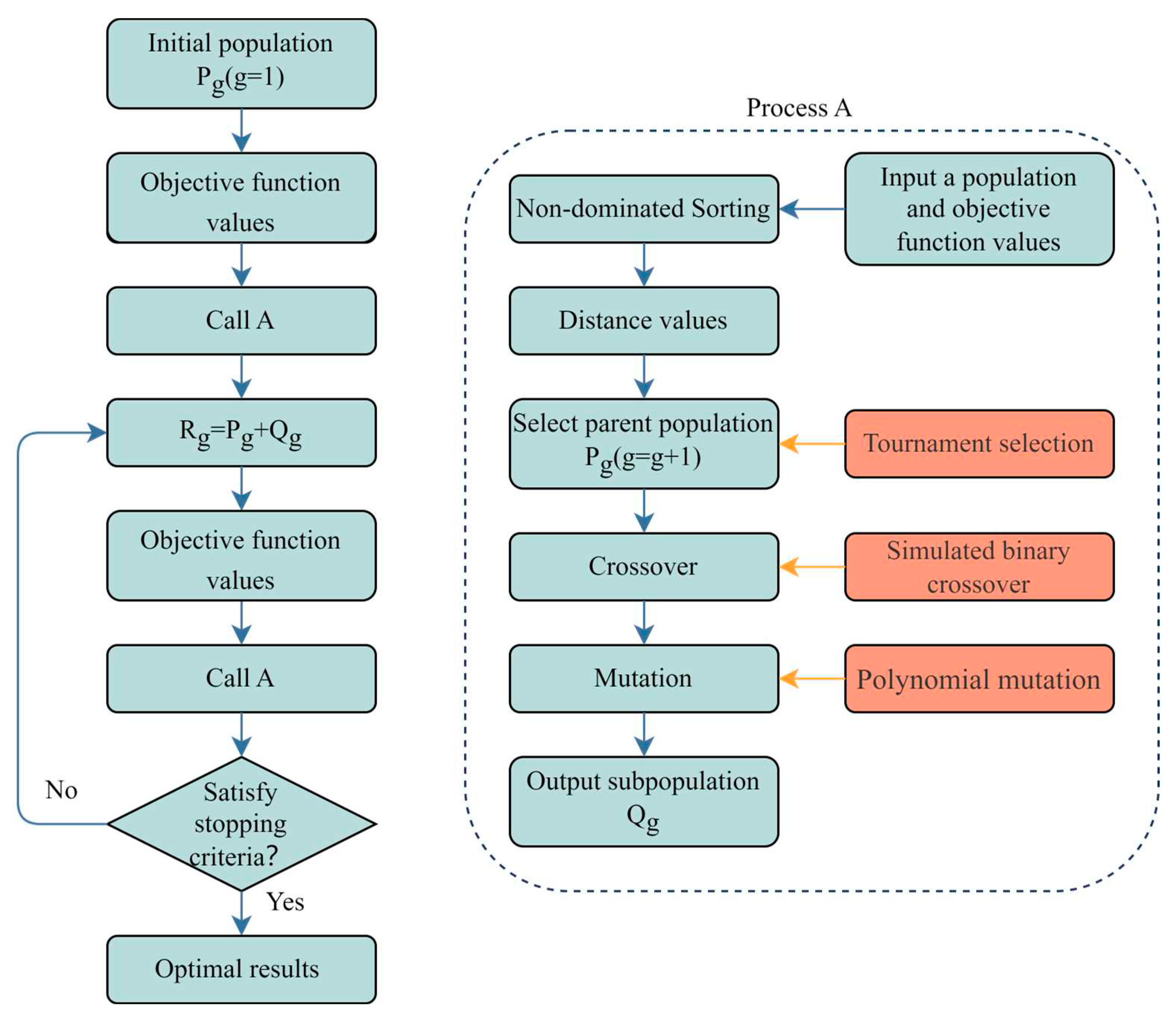
Figure 1. Flowchart of NSGA-II.
Preprints 82758 g001
Figure 2. Latin square.
Preprints 82758 g002
Figure 3. Optimization flowchart.
Preprints 82758 g003
Figure 4. Illustration of the Non-isothermal convection case.
Preprints 82758 g004
Figure 5. The change curve about F'min (Part A:Based on simulation data and 2D simulations; Part B:Based on experimental data and 3D simulations).
Preprints 82758 g005
Figure 6. The Pareto frontiers in three situations.
Preprints 82758 g006
Figure 7. Samples distribution.
Preprints 82758 g007
Figure 8. Samples distribution and its response values F1 (0.7 < Vin < 0.8 m/s; 16.0 < Tin < 17.5 ℃).
Preprints 82758 g008
Figure 9. Samples Distribution.
Preprints 82758 g009
Figure 10. 3D model of the dual-aisle single-row cabin.
Preprints 82758 g010
Figure 11. The change curve about F'min.
Preprints 82758 g011
Figure 12. Pareto Frontier.
Preprints 82758 g012
Figure 13. Three main types of airflow organization (A/B/C corresponds to solutions 1/3/9 in Table 5).
Preprints 82758 g013
Table 1. Some of the newest studies on air conditioning.
Methods Authors Other tools Situations
CFD-based adjoint Zhao, X. et al. (2018) [16] The centroid-based hierarchical cluster analysis Steady-state and single-objective
Artificial neural networks (ANN) Li, L. et al. (2023) [17] Particle swarm optimizer-grey wolf optimization Transient and multi-objective
Lin, C. J. et al. (2022) [18] Whale optimization algorithm Steady-state and multi-objective
Hou, F. et al. (2022) [19] Grey wolf optimization Steady-state and multi-objective
Ye, X. et al. (2022) [20] Technique for order preference by similarity to an ideal solution (TOPSIS) Steady-state and multi-objective
Li, L. et al. (2022) [21] PSO Steady-state and single-objective
Aruta, G. et al. (2023) [22] Non-dominated sorting genetic algorithm-II (NSGA-II) Multi-objective
Proper orthogonal decomposition (POD) Wang, X. et al. (2021) [23] Radial basis functions Steady-state and multi-objective
Liu, Y. et al. (2021) [24] Steady-state and multi-objective
Multi-step joint optimization Shao, X. et al. (2023) [25] Three flow field characteristic indicators Transient and multi-objective
Meta-heuristic optimization approaches Baba, F. M. et al. (2023) [26] NSGA-II Steady-state and multi-objective
Fan, Z. et al. (2022) [27] Improving the strength Pareto evolutionary algorithm-2 (SPEA-2) Steady-state and multi-objective
Rafati, N. et al. (2023) [28] NSGA-II Multi-objective
Wang, Y. et al. (2022) [29] NSGA-II and K-means Multi-objective
Mostafazadeh, F. et al. (2023) [30] NSGA-III and TOPSIS Multi-objective
Li, C. et al. (2023) [31] PSO Steady-state and single-objective
Sun, R. et al. (2023) [32] Genetic algorithm Steady-state and single-objective
Orthogonal experiment designs Yin, Y. et al. (2023) [33] Steady-state and single-objective
Chen, M. et al. (2023) [34] Steady-state and single-objective
Table 2. Pareto set and the objective function values.
NO. Vin (m/s)
(deviation)
Tin (℃) (deviation) F1 F2 F'
1 0.57103 (0.18%) 15.0359 (0.24%) 0.000151
(min)
0.001755 0.000953
(min)
2 0.55203 (3.15%) 14.9596 (0.29%) 0.005745 0.000493
(min)
0.003119
Notes: Based on simulation data and 2D simulations.
Table 3. Part of Pareto solutions and the objective function values.
NO. Vin (m/s)
(deviation)
Tin (℃) (deviation) F1 F2 F'
Iteration 39 (continuous) 1 0.61033 (7.075%) 16.43050 (9.53%) 0.05569
(min)
0.02771 0.04170
(min)
2 0.72669 (27.5%) 16.63695 (10.9%) 0.13114 0.01539
(min)
0.07327
Iteration 52 (continuous) 1 0.61394 (7.71%) 16.81935 (12.1%) 0.05531
(min)
0.02688 0.04109
2 0.55865 (1.99%) 16.64436 (11.0%) 0.05667 0.02359 0.04013
(min)
3 0.72669 (27.5%) 16.63695 (10.9%) 0.13114 0.01539
(min)
0.07327
Iteration 12 (discrete) 1 0.59
(3.51%)
16.5
(10.0%)
0.05497
(min)
0.02654 0.04075 (min)
2 0.76
(33.3%)
16.6
(10.7%)
0.12294 0.01565
(min)
0.06930
1 0.61033 (7.075%) 16.43050 (9.53%) 0.05569
(min)
0.02771 0.04170
(min)
Notes: Based on experimental data and 3D simulations.
Table 4. Range and precision of parameters.
Parameters Lower limit Upper limit Precision
t (℃) 8 20 0.1
V1 (m/s) 0.1 1.5 0.01
V2 (m/s) 0.1 1.5 0.01
θ1 (°) -80 80 1
θ2 (°) -80 80 1
Table 5. Part of Pareto solutions and the corresponding volume values.
NO. t (℃) V1 (m/s) V2 (m/s) θ1 (°) θ2 (°) volume1 (m3) volume2 (m3) total (m3)
1 8 0.76 0.98 19 12 0.786 0.709 (max) 1.496
2 10.8 0.83 0.29 -56 -15 1.236 0.621 1.856
3 10.8 0.87 0.28 -57 -17 1.296 0.596 1.893 (max)
4 10.6 0.9 0.27 -55 -20 1.301 0.578 1.880
5 11 0.87 0.31 -60 -14 1.304 0.550 1.854
6 10.9 0.86 0.29 -58 -17 1.305 0.549 1.854
7 10.9 0.87 0.29 -59 -15 1.316 0.526 1.841
8 10.8 0.86 0.31 -59 -17 1.340 0.495 1.834
9 9.8 1.01 0.97 -72 -68 1.371 (max) 0.394 1.765
Notes: Volume1 (2) refers to the volume in controlled area 1 (2) that satisfies |PMV|<0.5, and the total volume of controlled area 1 (2) is 1.47 (0.73) m3.
Table 6. A summary of the three methods (with multiple parameters).
CFD-based genetic algorithms POD method Surrogate-based
(this paper)
Target number (achievable) multiple multiple multiple
Target number
(current study)
multiple single double
Initial sample size small large medium
Sampling method random uniform/orthogonal experimental design Latin hypercube sampling technique
Randomness existent non-existent existent
Continuity assumption non-existent existent existent
Prediction process non-existent interpolation interpolation
Prediction method non-existent spline/polynomial/
radial basis function
Kriging
Gradient dependence non-existent existent existent
Database update existent usually non-existent existent
Subgeneration generation tool three kinds of operators usually non-existent infill criteria and NSGA-II
Number of new individuals usually equal to the initial sample size usually non-existent few
Validation times many one or few many
Effect of outliers non-existent existent existent
Costs higher medium lower
Disclaimer/Publisher’s Note: The statements, opinions and data contained in all publications are solely those of the individual author(s) and contributor(s) and not of MDPI and/or the editor(s). MDPI and/or the editor(s) disclaim responsibility for any injury to people or property resulting from any ideas, methods, instructions or products referred to in the content.
Copyright: This open access article is published under a Creative Commons CC BY 4.0 license, which permit the free download, distribution, and reuse, provided that the author and preprint are cited in any reuse.
Prerpints.org logo

Preprints.org is a free preprint server supported by MDPI in Basel, Switzerland.

Subscribe

© 2024 MDPI (Basel, Switzerland) unless otherwise stated