ASISO: A Robust and Stable Data Synthesis Method to Optimize Samples

Most existing data synthesis methods are designed to tackle problems such as dataset imbalance, data anonymization and insufficient sample size. There is a lack of effective synthesis methods for the limited number of datasets which contain a large of features and unknown noise to expand the size of the dataset. We propose a data synthesis method, named Adaptive Subspace Interpolation for Sample Optimization (ASISO). The idea is to divide the original feature space into several subspaces with an equal number of samples, and then perform interpolation for the samples in the adjacent subspaces. This method can adaptively adjust the size of the dataset containing unknown noise, and the expanded data typically contain minimal error with actual. Moreover, it adjusts the structure of the samples, which can significantly reduce the proportion of samples with large errors. In addition, the hyperparameters of this method have an intuitive explanation and usually require little calibration. Experimental results on artificial data and benchmark data sets demonstrate that ASISO is a robust and stable method to optimize samples.

Keywords:

Subject: Computer Science and Mathematics - Probability and Statistics

MSC: 6211; 68T09

1. Introduction

Synthetic data presents an effective solution to the challenges of inadequate or low-quality sample, particularly in the era of big data. Through the use of data synthesis methods to generate synthetic data, it provides a cost-effective and efficient alternative to collecting and labeling large amounts of real-world data. Furthermore, these methods can address privacy concerns associated with real-world data, making it safer to share and analyze [1]. Recently, there has been a surge in the use of synthetic data in machine learning, with various synthetic methods being developed [2,3].

Representative data synthesis methods can be classified into three categories. The first category entails techniques such as interpolation, extrapolation, and other methods [4] that generate additional data points representative of the underlying distribution. These methods improve the quality of the dataset and model generalization. For image data, deep learning-based methods such as VAE and GAN can also be used to generate new data [5,6]. These methods are useful for improving the quality of the dataset and model generalization. The second category is to address the issue of dataset imbalance, such as SMOTE [7], and some of its enhancements [8,9,10]. These methods can synthesize minority class samples to balance the dataset and improve the model’s performance. Finally, data sharing and research require sensitive data privacy protection. Synthetic data can help protect sensitive information while still enabling data sharing and research. Normally, we can add random noise to protect original data, generating synthetic data for sharing and research purposes like differential privacy methods [11]. Overall, these methods help optimize the representation and use of data in various applications.

For some actual tasks, original data often contains a multitude of features and unknown noise [12]. Since synthetic method involves generating new data based on existing data, the quality of the new points depends on the quality and quantity of the original data. If the quality of the original data is poor or the quantity is insufficient, then the synthetic data may have limitations in terms of its quality [13]. However, there exists a lack of effective synthetic methods for datasets with a restricted size and complex noise to expand the size of data set.

Based on the purpose of improving the quality and quantity of the dataset, and motivated by piecewise linear interpolation and spline interpolation, we propose a robust and stable data synthesis method named Adaptive Subspace Interpolation for Sample Optimization (ASISO), which aims to adaptively adjust the sample size and structure of the original dataset containing unknown noise. The idea is to divide the original feature space into several subspaces with an equal number of samples, and then perform linear interpolation for the samples in the adjacent subspaces. This method achieves sample optimization in two aspects. First, it can adaptively adjust the size of the dataset, and the expanded data typically contains minimal error with actual. Second, it adjusts the structure of the samples, which can significantly reduce the proportion of samples with large errors, thereby minimizing the impact of noise for model generalization.

The rest of this paper is organized as follows. Section 2 reviews the research of existing interpolation. Section 3 details the concept of the proposed ASISO method and provides proof for the effectiveness of this method. Experimental results are presented and analyzed in Section 4. Finally, we conclude this paper in Section 5.

2. Related Work

Traditional interpolation methods are based on the function values of known data points for extrapolation and prediction. For a given data set, there are generally two cases. In the case of two known data points and interpolation in between, interpolation can be selected based on distance, such as nearest-neighbor interpolation [14]. If it is assumed that the unknown point between these two data points is consistent with the straight line between them, a linear function can be used to fit and interpolate, such as linear interpolation, piecewise linear interpolation [15,16]. For interpolation among multiple given points, a commonly used method is to predict the value of the unknown point by constructing a high-degree polynomial based on the given points, such as Lagrange interpolation, Newton interpolation [17,18]. However, with an increase in the number of data points and the degree of the polynomial, there is a risk of overfitting and numerical instability (Runge’s phenomenon) [19]. Another solution is to construct a global smooth function by fitting a low-degree polynomial in a local region. In comparison to high-degree polynomial interpolation methods, this method has better smoothness and numerical stability, such as spline interpolation [20]. Nevertheless, as it is necessary to fit multiple local low-degree polynomials, this method can lead to relatively high computational complexity.

When expanding the sample size using interpolation methods, the selection of node positions and quantities has a significant impact on the accuracy and stability of interpolation results. Typically, equidistant nodes [21] are used for interpolation position selection, where nodes are equally spaced within the interpolation interval. Chebyshev nodes [22] are selected within the interpolation interval to satisfy certain conditions for better fitting of the function. In addition, the choice of the number of interpolations can lead to instability of the data and insufficient validation accuracy. One way to determine the appropriate number of interpolations is by comparing the fitting degree of the model trained under different interpolation numbers with the original data, but this may lead to overfitting and poor generalization ability of the model.

3. Proposed Method

In this section, we will explain the proposed ASISO method in detail. ASISO introduces two algorithms: K-Space and K-Match. To clearly illustrate the proposed method, we will first provide an overview of ASISO and then introduce the specific algorithms involved.

3.1. Overview

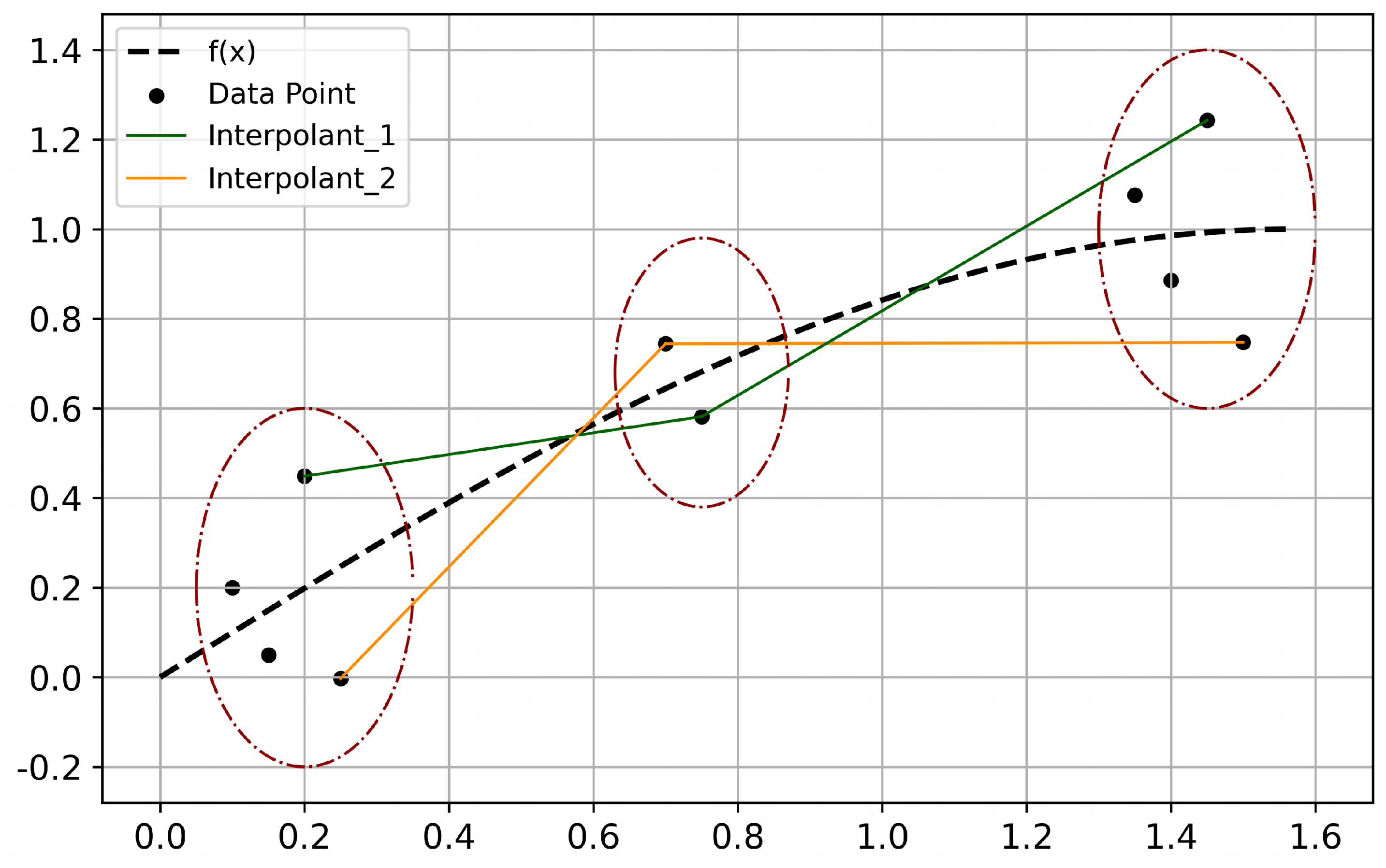
The ASISO is mainly based on the linear interpolation to increase the size and improve the quality of the original dataset. The idea is to divide the original feature space into several subspaces with an equal number of samples, and then perform linear interpolation for the samples in the adjacent subspaces. This method requires two hyperparameters (k and

η

) in advance. Interpretation of parameter k is the number of samples existing in each feature subspace, while

η

is the number of equidistant nodes interpolated per unit distance in the linear interpolation of the samples. This proposed method is illustrated in Figure 1.

The data set

D = {x_{i}, y_{i}}_{i = 1}^{n}

has been given and is assumed to be contaminated with unknown noise, where

x_{i} \in X = R^{p}

and

y_{i} \in Y = R

. Assuming

{\dot{y}}_{i} = f ({\dot{x}}_{i})

where

{\dot{x}}_{i}

is the actual value of

x_{i}

{\dot{y}}_{i}

is the actual value of

y_{i}

and

f (\cdot)

is a continuous function, represents the relationship in reality between

x_{i}

and y. Consider the model:

{\dot{y}}_{i} + ϵ_{i, y} = f ({\dot{x}}_{i} + ϵ_{i, x}) + ϵ_{i},

(1)

where

ϵ_{i, y}

is the noise in

{\dot{y}}_{i}

ϵ_{i, x}

is the noise in

{\dot{x}}_{i}

, and

ϵ_{i}

represents the error term. The expression (1) can be rewritten as:

y_{i} = f (x_{i}) + ϵ_{i} .

(2)

Let

x_{0} = {x_{0}^{1}, \dots, x_{0}^{p}}

, we have

x_{0}^{j} = i n f {x_{i}^{j}}_{i = 1}^{n}

for

\forall j = 1, \dots, p

, and call

x_{0}

the sample minimum point.

Given the hyperparameter k, we provide an unsupervised clustering method called K-Space. As it is shown in Figure 1(b), the space can be partitioned into

n / k

subspaces, each containing k samples. i.e.,

X = \cup_{s = 1}^{n / k} X_{s}

X_{i} \cap X_{j} = \emptyset, i, j = 1, 2, \dots, \frac{n}{k}

and

i \neq j

. The datasets corresponding to different subspaces

D = \cup_{s = 1}^{n / k} D_{s}, D_{s} = {(x_{i}^{s}, y_{i}^{s})}_{i = 1}^{k}

x_{i}^{s} \in X_{s}

. For two adjacent subspaces, since

f (\cdot)

is a continuous function, we assume that it can be approximated as a linear function

g (\cdot)

, and then (2) can be transformed into:

y_{i} = g (x_{i}) + ϵ_{i} + ϵ_{i}^{'},

(3)

where

ϵ_{i}^{'}

is the linear fitting error term. When the distance between two adjacent subspaces approaches zero and the measurements of subspaces tend to zero, obtain

ϵ_{i}^{'} \to 0

. Next, we will perform sample interpolation between adjacent subspaces.

We need to calculate the centers of each cluster, as follow:

{\bar{x}}^{s} = \frac{1}{k} \sum_{x_{i}^{s} \in D_{s}} x_{i}^{s} .

(4)

To make

ϵ_{i}^{'} \to 0

, we need to ensure that the interpolation is performed between clusters that are close in distance as much as possible. Among

{D_{s}}_{s = 1}^{n / k}

, we define

D_{(1)}

whose cluster center has the minimum distance to the sample minimum point

x_{0}

, and define

D_{(d)}

whose cluster center has the minimum distance to the center of

D_{(d - 1)}, D_{(d - 1)} \neq D_{(1)}, \dots, D_{(d - 1)}

and

d > 1

D_{(1)} = \underset{D_{s} \in D}{a r g m i n} d i s t (x_{0}, {\bar{x}}^{s}),

(5)

D_{(d)} = \underset{{D_{s} \in D}, D_{s} \neq D_{(1)}, \dots, D_{(d - 1)}}{a r g m i n} d i s t ({\bar{x}}_{0}^{(d - 1)}, {\bar{x}}^{s}),

(6)

where

{\bar{x}}^{(d - 1)}

is the center of

D_{(d - 1)}

. Perform interpolation in

{D_{(d)}}_{d = 1}^{n / k}

sequentially according to the order of d values, and interpolate only between adjacent subspaces (i.e., interpolate between

D_{(1)}

and

D_{(2)}

, between

D_{(2)}

and

D_{(3)}

, and so on).

When performing linear interpolation between adjacent subspaces, we should pair the k samples from the first subspace with an equal number of samples from the second subspace. The interpolation rules between adjacent subspaces are as follows:

1. Linear interpolation can only be performed between two samples belonging to different adjacent subspace sets.

2. Interpolation must be performed for each sample.

3. Participation of each sample point is restricted to a single interpolation instance.

The number of matching schemes is

k!

. As it is shown in Figure 1(c), we provide a matching method called K-Match. Suppose

ϵ_{i}^{'} \to 0

, this method can select a good-performing matching scheme

{(x_{i}^{(d)}, y_{i}^{(d)}), (x_{i}^{(d + 1)}, y_{i}^{(d + 1)})}_{i = 1}^{k}

from

k!

Assuming

x

and y are continuous variables. Given another hyperparameter

η

, the number of samples inserted using linear interpolation method between

D_{(d)}

and

D_{(d + 1)}

\sum_{i = 1}^{k} ⌊ η \cdot d i s t (x_{i}^{(d)}, x_{i}^{(d + 1)}) ⌋

. Taking

(x_{i}^{(d)}, y_{i}^{(d)}) \in D_{(d)}

and

(x_{i}^{(d + 1)}, y_{i}^{(d + 1)}) \in D_{(d + 1)}

as example,

{(x_{(d, d + 1)}^{(m, i)},

y_{(d, d + 1)}^{(m, i)} {)}}_{m = 1}^{⌊ η \cdot d i s t (x_{i}^{(d)}, x_{i}^{(d + 1)}) ⌋}

is the set of inserted samples, the linear interpolation formula is defined as:

x_{(d, d + 1)}^{(m, i)} = x_{i}^{(d)} + m \cdot \frac{x_{i}^{(d + 1)} - x_{i}^{(d)}}{⌊ η \cdot d i s t (x_{i}^{(d)}, x_{i}^{(d + 1)}) ⌋ + 1},

(7)

y_{(d, d + 1)}^{(m, i)} = y_{i}^{(d)} + m \cdot \frac{y_{i}^{(d + 1)} - y_{i}^{(d)}}{⌊ η \cdot d i s t (y_{i}^{(d)}, y_{i}^{(d + 1)}) ⌋ + 1} .

(8)

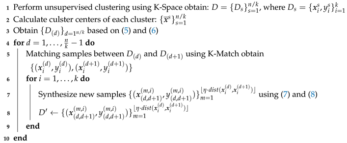
After ASISO processing, the original dataset will be optimized. The main steps of the ASISO algorithm are summarized in Algorithm 1.

Algorithm 1: ASISO

Input: Data set

D = {{(x_{i}, y_{i}}}_{i = 1}^{n}

; hyperparameters k and

η

Output: Optimized data set

D^{'}

The assumptions of ASISO are as follows:

f (\cdot)

is a continuous function.

2. the linear fitting error

ϵ_{i}^{'} \to 0

x

and y are continuous variables.

3.2. K-Space

The implementation of ASISO requires an unsupervised clustering method to partition the feature space into multiple subspaces, each containing k samples. Based on this, we propose the K-Space clustering method. The clustering method has the following performance:

1.Each subspace contains an equal number of samples, i.e.,

D = \cup_{s = 1}^{n / k} D_{s}, D_{s} = {(x_{i}^{s}, y_{i}^{s})}_{i = 1}^{k}

;

2.Each sample belongs to only one subset, i.e.,

D_{i} \cap D_{j} = \emptyset, i \neq j

Maintaining continuity and similarity between adjacent subspaces is essential for synthesizing data via multiple linear interpolations in ASISO. Our objective is to minimize the linear fitting error

ϵ_{i}^{'}

, which helps to satisfy ASISO assumption 2 as much as possible.

To determine the sample set

D_{s}

for subspace

X_{s}

, it is necessary to determine the first sample

x_{1}^{s}

D_{s}

x_{1}^{s} = \underset{x : x \in D, x \notin D_{1}, \dots, D_{s - 1}}{a r g m i n} d i s t (x, {\bar{x}}^{s - 1}),

(9)

where

s = 1, \dots, \frac{n}{k}

{\bar{x}}^{s - 1}

is the cluster center of

D_{s - 1}

{\bar{x}}^{0} = x_{0}

. We define

D_{s} = {x_{1}^{s}}

and determine

x_{d}^{s}

as follows:

x_{d}^{s} = \underset{x : x \in D, x \notin D_{1}, \dots, D_{s}}{a r g m i n} d i s t (x, {\bar{x}}^{s}),

(10)

where

d = 2, \dots, k

. Obtain

x_{d}^{s}

and update

D_{s} \leftarrow D_{s} \cup {x_{d}^{s}}

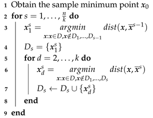
The main steps of the K-Space algorithm are summarized in Algorithm 2.

Algorithm 2: K-Space

Input: Data set

D = {(x_{i}, y_{i})}_{i = 1}^{n}

; hyperparameter k

Output:

{D_{s}}_{s = 1}^{n / k}

3.3. K-Match

We can calculate the total error of the matching scheme to measure the quality of the scheme, for the sake of simplicity, let

X = R

, as follow:

\sum_{i = 1}^{k} S (x_{i}^{(d)}, x_{i}^{(d + 1)}) = \sum_{i = 1}^{k} \int_{x_{i}^{(d)}}^{x_{i}^{(d + 1)}} | f (x) - L_{i} (x) | d x,

(11)

where

L_{i} (x)

is the linear expression passing through the points

(x_{i}^{(d)}, y_{i}^{(d)})

and

(x_{i}^{(d + 1)}, y_{i}^{(d + 1)})

Theorem 1.

Let

X_{(d)}

and

X_{(d + 1)}

be two adjacent subspaces, the datasets corresponding to different subspaces are

D_{(d)}, D_{(d + 1)}

, and

(x_{i}^{(d)}, y_{i}^{(d)}) \in D_{(d)}, (x_{i}^{(d + 1)}, y_{i}^{(d + 1)}) \in D_{(d + 1)}

. Consider the model

y_{i} = f (x_{i}) + ϵ_{i}

, let

ϵ_{i}^{(d)} = y_{i}^{(d)} - f (x_{i}^{(d)})

. For

\forall i = 1, 2, \dots, k

, suppose that

ϵ_{i}^{'} \to 0

, then

E (\frac{S (x_{i}^{(d)}, x_{i}^{(d + 1)})}{| x_{i}^{(d)} - x_{i}^{(d + 1)} |}) < E (\frac{| ϵ_{i}^{(d)} | + | ϵ_{i}^{(d + 1)} |}{2})

Proof of Theorem 1.

Since

ϵ_{i}^{'} \to 0

, and according to (3), the model can be transformed into:

y_{i} = g (x_{i}) + ϵ_{i},

where

g (\cdot)

is a linear function. According to (11), it follows that:

S (x_{i}^{(d)}, x_{i}^{(d + 1)}) = \int_{x_{i}^{(d)}}^{x_{i}^{(d + 1)}} | g (x) - L_{i} (x) | d x .

When

ϵ_{i}^{(d)} \cdot ϵ_{i}^{(d + 1)} < 0

, let

(x^{'}, y^{'})

be the intersection point between

y = L_{i} (x)

and

y = g (x)

. We can simplify

S (x_{i}^{(d)}, x_{i}^{(d + 1)})

using basic geometric area calculations, and according to Law of Iterated Expectations (LIE):

\begin{matrix} E (\frac{S (x_{i}^{(d)}, x_{i}^{(d + 1)})}{| x_{i}^{(d)} - x_{i}^{(d + 1)} |}) & = \frac{E (S (x_{i}^{(d)}, x_{i}^{(d + 1)}) | ϵ_{i}^{(d)} \cdot ϵ_{i}^{(d + 1)} \geq 0) P (ϵ_{i}^{(d)} \cdot ϵ_{i}^{(d + 1)} \geq 0)}{| x_{i}^{(d)} - x_{i}^{(d + 1)} |} \\ + \frac{E (S (x_{i}^{(d)}, x_{i}^{(d + 1)}) | ϵ_{i}^{(d)} \cdot ϵ_{i}^{(d + 1)} < 0) P (ϵ_{i}^{(d)} \cdot ϵ_{i}^{(d + 1)} < 0)}{| x_{i}^{(d)} - x_{i}^{(d + 1)} |} \\ = \frac{E (| ϵ_{i}^{(d)} | + | ϵ_{i}^{(d + 1)} |) P (ϵ_{i}^{(d)} \cdot ϵ_{i}^{(d + 1)} \geq 0)}{2} \\ + \frac{(h_{1} \cdot E | ϵ_{i}^{(d)} | + h_{2} \cdot E | ϵ_{i}^{(d + 1)} |) P (ϵ_{i}^{(d)} \cdot ϵ_{i}^{(d + 1)} < 0)}{2}, \end{matrix}

where

h_{1} = \frac{| x^{'} - x_{i}^{(d)} |}{| x_{i}^{(d)} - x_{i}^{(d + 1)} |}, h_{2} = \frac{| x^{'} - x_{i}^{(d + 1)} |}{| x_{i}^{(d)} - x_{i}^{(d + 1)} |}

. Since

P (ϵ_{i}^{(d)} \cdot ϵ_{i}^{(d + 1)} \geq 0) + P (ϵ_{i}^{(d)} \cdot ϵ_{i}^{(d + 1)} < 0) = 1

, and

h_{1} + h_{2} = 1

, it follows that

E (\frac{S (x_{i}^{(d)}, x_{i}^{(d + 1)})}{| x_{i}^{(d)} - x_{i}^{(d + 1)} |}) < E (\frac{| ϵ_{i}^{(d)} | + | ϵ_{i}^{(d + 1)} |}{2})

□

If our approach is to randomly select a matching scheme, the validity of this method can be proved by Theorem 1. However, randomly selecting a matching scheme does not guarantee the uniqueness of the results, and it also does not guarantee that we will necessarily select the good-performing matching scheme. We found that for

x_{i}^{(d)}

and

x_{i}^{(d + 1)}

, if

ϵ_{i}^{(d)} \cdot ϵ_{i}^{(d + 1)} < 0

, there will be a better interpolation effect.

Theorem 2.

Let

y_{i}^{(d)} = f (x_{i}^{(d)}) + ϵ_{i}^{(d)}, y_{i}^{(d + 1)} = f (x_{i}^{(d + 1)}) + ϵ_{i}^{(d + 1)}

. Suppose that

ϵ_{i}^{'} \to 0

, then we have

E (S (x_{i}^{(d)}, x_{i}^{(d + 1)}) | ϵ_{i}^{(d)} \cdot ϵ_{i}^{(d + 1)} < 0) < E (S (x_{i}^{(d)}, x_{i}^{(d + 1)}) | ϵ_{i}^{(d)} \cdot ϵ_{i}^{(d + 1)} \geq 0)

Proof of Theorem 2.

Since

ϵ_{i}^{'} \to 0

, based on the proof of theorem 1, we have:

\begin{matrix} E (S (x_{i}^{(d)}, x_{i}^{(d + 1)}) | ϵ_{i}^{(d)} ϵ_{i}^{(d + 1)} \geq 0) \\ = \frac{| x_{i}^{(d)} - x_{i}^{(d + 1)} | \cdot E | ϵ_{i}^{(d)} | + | x_{i}^{(d)} - x_{i}^{(d + 1)} | \cdot E | ϵ_{i}^{(d + 1)} |}{2}, \end{matrix}

\begin{matrix} E (S (x_{i}^{(d)}, x_{i}^{(d + 1)}) | ϵ_{i}^{(d)} ϵ_{i}^{(d + 1)} < 0) \\ = \frac{| x^{'} - x_{i}^{(d)} | \cdot E | ϵ_{i}^{(d)} | + | x^{'} - x_{i}^{(d + 1)} | \cdot E | ϵ_{i}^{(d + 1)} |}{2} . \end{matrix}

It follows that

\begin{matrix} E (S (x_{i}^{(d)}, x_{i}^{(d + 1)}) | ϵ_{i}^{(d)} ϵ_{i}^{(d + 1)} < 0) < E (S (x_{i}^{(d)}, x_{i}^{(d + 1)}) | ϵ_{i}^{(d)} ϵ_{i}^{(d + 1)} \geq 0) . \end{matrix}

□

According to Theorem 2, we can match samples with opposite signs of

ϵ_{i}

to achieve a good data synthesis effect. Therefore, the core idea of K-match is to make a judgment on the positive or negative sign of

ϵ_{i}

for each sample, and then interpolate the samples with opposite signs as much as possible.

In K-Match, we need to choose an appropriate linear regression method to fit the dataset

D_{(d)} \cup D_{(d + 1)}

based on the performance of the noise. For example, Lasso regression, Locally Weighted Linear Regression (LWLR) [23], and other methods can be used [24,25]. In our experiments, we use OLS or SVR method to fit and obtain

\hat{g} (\cdot)

. Specially, the kernel function is Linear in SVR. According to (3), and suppose the linear fitting error

ϵ_{i}^{'} \to 0

, for dataset

D_{(d)} \cup D_{(d + 1)}

, we have:

ϵ_{i} = y_{i} - \hat{g} (x_{i}) .

(12)

Then, we sort the samples in dataset

D_{(d)}

in ascending order according to the value of

ϵ_{i}

, and obtain

{(x_{i}^{(d)}, y_{i}^{(d + 1)})}_{i = 1}^{k}

; we sort the samples in dataset

D_{(d + 1)}

in descending order and obtain

{(x_{i}^{(d + 1)}, y_{i}^{(d + 1)})}_{i = 1}^{k}

. As it is shown in Figure 1(d), combine the sorted datasets

D_{(d)}

and

D_{(d + 1)}

into the matching scheme

{(x_{i}^{(d)}, y_{i}^{(d)}), (x_{i}^{(d + 1)}, y_{i}^{(d + 1)})}_{i = 1}^{k}

Algorithm 3: K-Match

Input: Subset

D_{(d)} = {(x_{i}^{(d)}, y_{i}^{(d)})}_{i = 1}^{k}, D_{(d + 1)} = {{(x_{i}^{(d + 1)}, y_{i}^{(d + 1)}}}_{i = 1}^{k}

Output: Matching scheme

{(x_{i}^{(d)}, y_{i}^{(d)}), (x_{i}^{(d + 1)}, y_{i}^{(d + 1)})}_{i = 1}^{k}

1 Fitting the dataset

D_{(d)} \cup D_{(d + 1)}

and obtain

\hat{g} (\cdot)

2 Obtain

{ϵ_{i}}

using (10)

3 Sorting the samples in

D_{(d)}

and

D_{(d + 1)}

according to the value of

ϵ_{i}

, obtain

D_{(d)}^{'}

and

D_{(d + 1)}^{'}

4 Combine

D_{(d)}^{'}

and

D_{(d + 1)}^{'}

into

{(x_{i}^{(d)}, y_{i}^{(d)}), (x_{i}^{(d + 1)}, y_{i}^{(d + 1)})}_{i = 1}^{k}

3.4. Supplements

The proposed method can effectively expand the size of dataset and adjust the dataset structure, reducing the proportion of samples that deviate significantly from the actual distribution, thereby improving the model generalization. Refer to Figure 2.

The supplements about ASISO are given below:

1. The choice of the hyperparameter k is crucial as different datasets require different values of k. Conversely, hyperparameter

η

tends to exhibit better performance as its value increases, which will be illustrated in the following experimental results.

2. It is necessary to normalize the data if there is a significant difference in the dimensional scale between the features of the data. It avoids the issue of generating an excessive number of samples.

3. In most cases,

n / k

is not an integer, and for the excess samples, we usually have two solutions of handling them. The first one is to use the LOF algorithm [26] to filter out the excess samples that will not participate in the ASISO, as it is shown in Figure 2(c). Another solution is to treat the excess samples as a dataset

D^{'}

of a subspace,

D^{'} = {(x_{i}, y_{i})}_{i = 1}^{n m o d k}

.When interpolating between

D^{'}

and other subspaces

D^{''}

, choose an appropriate linear regression method to fit the dataset

D^{'} \cup D^{''}

, and obtain

\hat{g} (\cdot)

. Then, use the same method to sort

D^{'}

and

D^{''}

. Only

n m o d k

interpolations are performed, with each sample in

D^{'}

being interpolated, while for

D^{''}

, only

n m o d k

samples are interpolated. Moreover, interpolate the samples with opposite signs of

ϵ_{i}

as much as possible, as it is shown in Figure 3.

4. Experiments

For Artificial data, as

f (\cdot)

can be known, we investigated the hyperparameter selection, and optimization performance after processing by ASISO. For benchmark data, we studied the prediction performance using this method.

4.1. Artificial Data Sets

Some verification indicators, the proportion of samples with

ϵ_{i}

greater than

α

, and the mean square error (MSE), can be selected to test the optimization effect of the ASISO on the original sample after processing, as follows:

p (α) = \frac{1}{n} \sum_{i = 1}^{n} I (| f (x_{i}) - y_{i} | > α),

(13)

M S E = \frac{1}{n} \sum_{i = 1}^{n} {(f (x_{i}) - y_{i})}^{2} .

(14)

For artificial data sets,

{x_{i}}_{i = 1}^{n}

are generated by

N_{p} (0, E)

. Let

W_{1} \in R_{(p \times p_{1})}

and

W_{2} \in R_{(p_{1} \times 1)}

, where all elements of both

W_{1}

and

W_{2}

are independently and identically distributed as

N (0, 1)

. Consider

y_{i} = f (x_{i}) + ϵ_{i} = t a n h (x_{i}^{'} W_{1}) W_{2} + ϵ_{i}

t a n h (x) = \frac{e^{x} - e^{- x}}{e^{x} + e^{- x}} .

For a given data set, we typically cannot ascertain the distribution of noise. Hence, we construct datasets that contain unknown noises [12]. The unknown noises are simulated by mixture noises that contain uniform noises and Gaussian noises. The generation of

ϵ_{i}

referenced to [27]. We have fixed the random effects of the generated datasets; experiments are repeated 100 times in each artificial dataset. Table 1 shows 6 artificial datasets.

4.1.1. Hyperparameter Selection

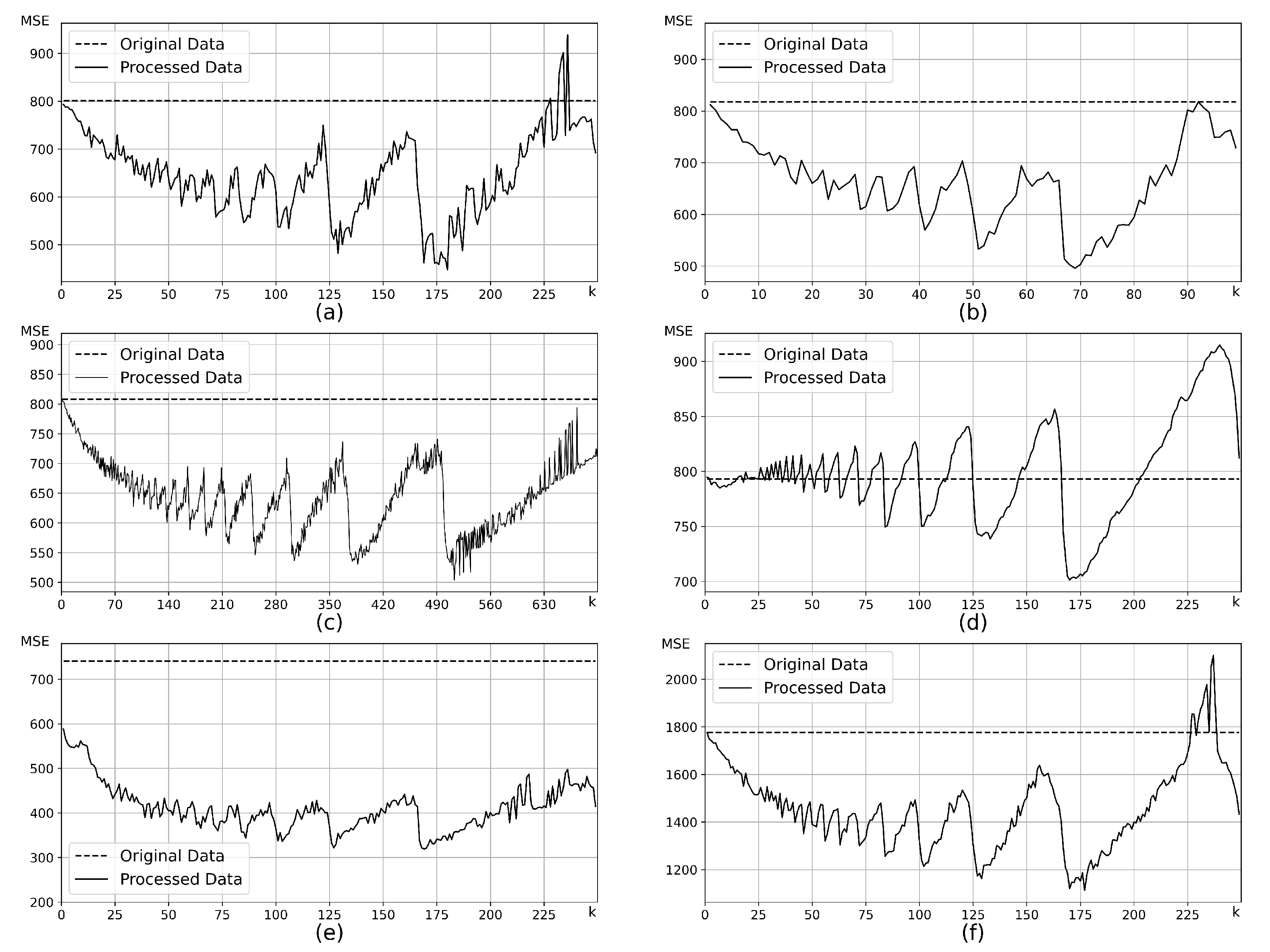
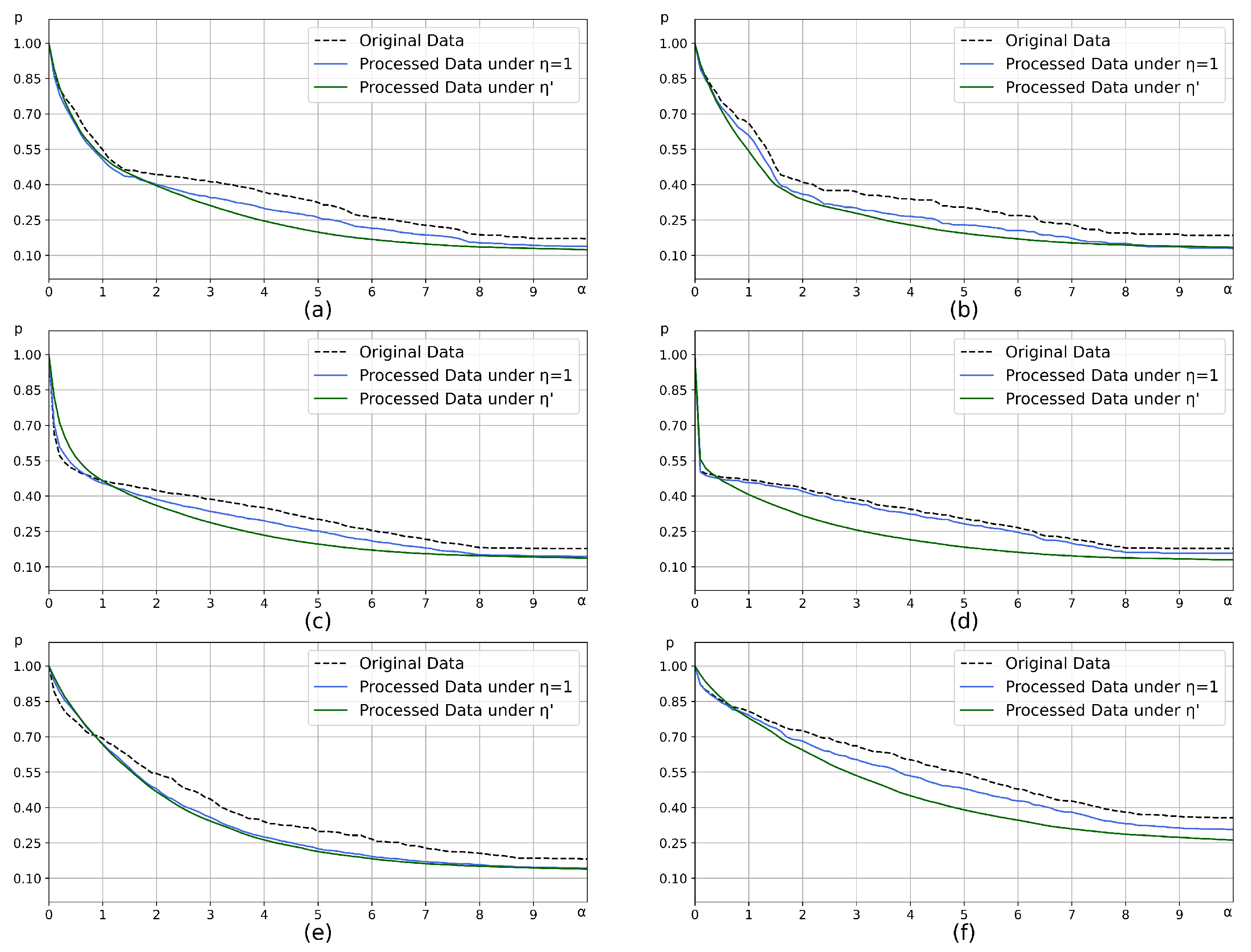
First, we investigate the selection of parameter k. To ensure that the number of feature subspaces is sufficient. We set the hyperparameter

η = 1

, let

k = 1, 2, \dots, ⌊ \frac{n}{2} ⌋

. Calculate the changes in MSE of the datasets at different values of k, obtain

k^{'} = \underset{k : k = 1, 2, \dots, ⌊ \frac{n}{2} ⌋, η = 1}{a r g m i n} M S E

. The change trend of the MSE index before and after the ASISO processing is shown in Figure 4. Then, let

η = 1, 2, \dots, 30, k = k^{'}

, calculate the changes in MSE of the datasets (Figure 5), obtain

η^{'} = \underset{η : η = 1, 2, \dots, 30, k = k^{'}}{a r g m i n} M S E

. At last, let

k = k^{'}, η = 1

and

η^{'}

, calculate the changes in

p (α)

of the artificial datasets (Figure 6).

As can be seen from Figure 4, ASISO demonstrates good optimization performance for datasets with varying sample sizes or feature dimensions. Experimental results also show that the performance of ASISO does not decline dramatically as the content of noise with large variances increases. Hence, it can deal with unknown noise better and has good robustness. In addition, it can be shown that ASISO exhibits good optimization performance for all datasets from experimental results, it is also a stable data synthesis method. As can be seen from Figure 5, the hyperparameter

η

has a generally monotonically decreasing relationship with MSE, and the larger the value of

η

, the more significant the effect. From Figure 6, it can be observed that ASISO can adaptively adjust the sample structure, which reduces the proportion of samples with large errors.

4.1.2. Comparison of Optimization Performance

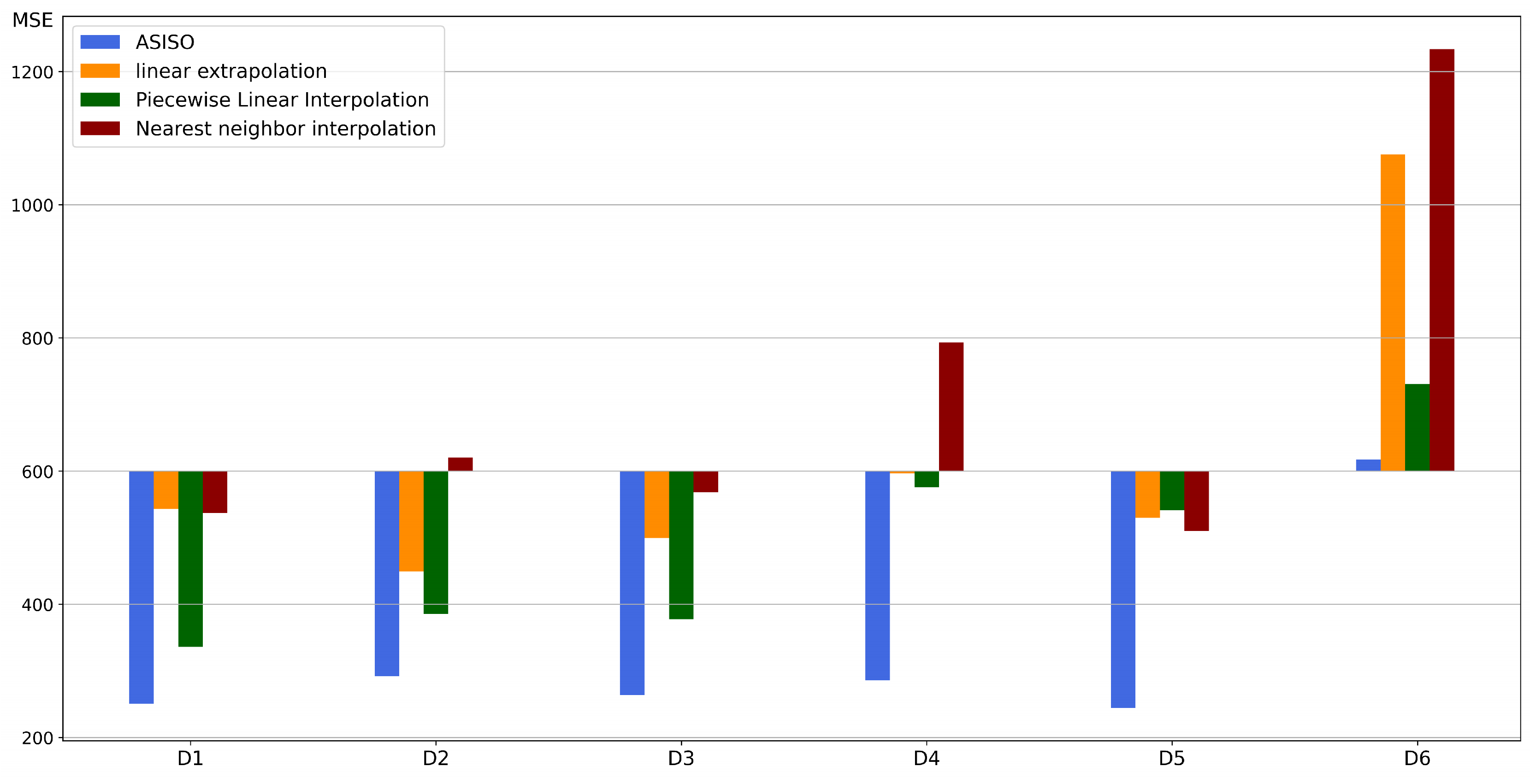
To verify the optimization performance of ASISO, it is compared three methods: piecewise linear interpolation, linear extrapolation, and nearest neighbor interpolation. Specifically, let

k = k^{'}, η = η^{'}

in ASISO. Based on the given dataset, we use the samples generated by ASISO as interpolation points to calculate the output values in linear extrapolation and nearest neighbor interpolation. Moreover, let

k = 1

and

η = η^{'}

in ASISO, we can regard it as piecewise linear interpolation. The experimental results show that ASISO has the smallest MSE among all methods for each dataset (Figure 7).

4.2. Benchmark Data Sets

To verify the prediction performance of ASISO, 4 benchmark data sets are used [28,29]. We partitioned the dataset into training and testing sets using a 7:3 ratio and normalize the data using the min-max normalization method. We preprocessed the training data using ASISO, train multiple machine learning models on the training set, and evaluated the prediction performance of the models on the testing set. The evaluation metric we used was mean absolute error (MAE).

M A E = \frac{1}{n} \sum_{i = 1}^{n} | y_{i} - {\hat{y}}_{i} | .

(15)

In addition, we removed features that cannot be directly used, such as “Datetime” for bike sharing demand, “Month” for forest fires, and so on. We choose K-Nearest Neighbor (KNN), Random Forest (RF), Gradient Boosting Decision Tree (GBDT), Multilayer Perceptron (MLP) and Support Vector Regression (SVR) as the machine learning prediction models. Specifically, the kernel function is Radial Basis Function (RBF) in SVR. Moreover, set the number of hidden layers to 3 for the MLP and use different numbers of neurons based on the input dimensionality and sample size.

The experimental results of the five models are shown in Table 2. It is evident that ASISO performs well on each benchmark dataset. This method is highly applicable to all five models, and in most cases, it can improve the predictive performance. It is worth mentioning that the dataset contains many categorical features, which are not continuous variables. Moreover, for sparse samples (Facebook Metrics and Forest Fires), it is difficult to guarantee that the linear fitting error

ϵ_{i}^{'} \to 0

when interpolating between subspaces. This indicates that even if there are violations of the ASISO assumptions in practical applications, this method may still achieve good optimization results. This further demonstrates that it is robust and stable.

5. Conclusions

In this paper, we propose a data synthesis method, ASISO, which can adaptively adjust the size of the dataset, and the expanded data typically contain minimal error with actual. Moreover, it can adjust the structure of the samples, which can significantly reduce the proportion of samples with large errors. The experimental results on artificial data sets demonstrate that ASISO can optimize the samples, and compared to other methods, the generated data using this method has smaller errors. It can deal with unknown noise better and has good robustness. The results on benchmark data sets show the proposed method is applicable to many machine models, and in most cases, it can improve the model generalization.

References

ALRikabi H T S, Hazim H T. Enhanced data security of communication system using combined encryption and steganography. iJIM, 2021, 15(16): 145. [CrossRef]
Kollias D. ABAW: learning from synthetic data & multi-task learning challenges. European Conference on Computer Vision. Cham: Springer Nature Switzerland, 2022: 157-172. [CrossRef]
Mahesh B. Machine learning algorithms-a review. International Journal of Science and Research (IJSR).[Internet], 2020, 9(1): 381-386.
Lepot M, Aubin J B, Clemens F H L R. Interpolation in time series: An introductive overview of existing methods, their performance criteria and uncertainty assessment. Water, 2017, 9(10): 796. [CrossRef]
Chlap P, Min H, Vandenberg N, et al. A review of medical image data augmentation techniques for deep learning applications. Journal of Medical Imaging and Radiation Oncology, 2021, 65(5): 545-563. [CrossRef]
Shorten C, Khoshgoftaar T M. A survey on image data augmentation for deep learning. Journal of big data, 2019, 6(1): 1-48. [CrossRef]
Chawla N V, Bowyer K W, Hall L O, et al. SMOTE: synthetic minority over-sampling technique. Journal of artificial intelligence research, 2002, 16: 321-357. [CrossRef]
Dablain D, Krawczyk B, Chawla N V. DeepSMOTE: Fusing deep learning and SMOTE for imbalanced data. IEEE Transactions on Neural Networks and Learning Systems, 2022. [CrossRef]
Han H, Wang W Y, Mao B H. Borderline-SMOTE: a new over-sampling method in imbalanced data sets learning.International conference on intelligent computing. Berlin, Heidelberg: Springer Berlin Heidelberg, 2005: 878-887. [CrossRef]
Bunkhumpornpat C, Sinapiromsaran K, Lursinsap C. Safe-level-smote: Safe-level-synthetic minority over-sampling technique for handling the class imbalanced problem. Advances in Knowledge Discovery and Data Mining: 13th Pacific-Asia Conference, PAKDD 2009 Bangkok, Thailand, April 27-30, 2009 Proceedings 13. Springer Berlin Heidelberg, 2009: 475-482. [CrossRef]
Ha T, Dang T K, Dang T T, et al. Differential privacy in deep learning: an overview. 2019 International Conference on Advanced Computing and Applications (ACOMP). IEEE, 2019: 97-102. [CrossRef]
Meng D, De La Torre F. Robust matrix factorization with unknown noise. Proceedings of the IEEE international conference on computer vision. 2013: 1337-1344. [CrossRef]
Raghunathan T E. Synthetic data. Annual review of statistics and its application, 2021, 8: 129-140. [CrossRef]
Sibson R. A brief description of natural neighbour interpolation. Interpreting multivariate data, 1981: 21-36.
Tachev G T. Piecewise linear interpolation with nonequidistant nodes. Numerical Functional Analysis and Optimization, 2000, 21(7-8): 945-953. [CrossRef]
Blu T, Thévenaz P, Unser M. Linear interpolation revitalized. IEEE Transactions on Image Processing, 2004, 13(5): 710-719. [CrossRef]
Berrut J P, Trefethen L N. Barycentric lagrange interpolation. SIAM review, 2004, 46(3): 501-517. [CrossRef]
Musial J P, Verstraete M M, Gobron N. Comparing the effectiveness of recent algorithms to fill and smooth incomplete and noisy time series. Atmospheric chemistry and physics, 2011, 11(15): 7905-7923. [CrossRef]
Fornberg B, Zuev J. The Runge phenomenon and spatially variable shape parameters in RBF interpolation. Computers & Mathematics with Applications, 2007, 54(3): 379-398. [CrossRef]
Rabbath C A, Corriveau D. A comparison of piecewise cubic Hermite interpolating polynomials, cubic splines and piecewise linear functions for the approximation of projectile aerodynamics. Defence Technology, 2019, 15(5): 741-757. [CrossRef]
Habermann C, Kindermann F. Multidimensional spline interpolation: Theory and applications. Computational Economics, bm2007, 30: 153-169. [CrossRef]
Ganzburg M I. The Bernstein constant and polynomial interpolation at the Chebyshev nodes. Journal of Approximation Theory, 2002, 119(2): 193-213. [CrossRef]
Cleveland W S. Robust locally weighted regression and smoothing scatterplots. Journal of the American statistical association, 1979, 74(368): 829-836. [CrossRef]
Lichti D D, Chan T O, Belton D. Linear regression with an observation distribution model. Journal of geodesy, 2021, 95: 1-14. [CrossRef]
Liu C, Li B, Vorobeychik Y, et al. Robust linear regression against training data poisoning. Proceedings of the 10th ACM workshop on artificial intelligence and security. 2017: 91-102. [CrossRef]
Breunig M M, Kriegel H P, Ng R T, et al. LOF: identifying density-based local outliers. Proceedings of the 2000 ACM SIGMOD international conference on Management of data. 2000: 93-104. [CrossRef]
Guo Y, Wang W, Wang X. A robust linear regression feature selection method for data sets with unknown noise. IEEE Transactions on Knowledge and Data Engineering, 2021, 35(1): 31-44. [CrossRef]
Cukierski W. Bike Sharing Demand. Kaggle, https://kaggle.com/competitions/bike-sharing-demand, 2014.
Dua D, Craff C. UCI Machine Learning Repository, http://archive.ics.uci.edu/ml, 2017.

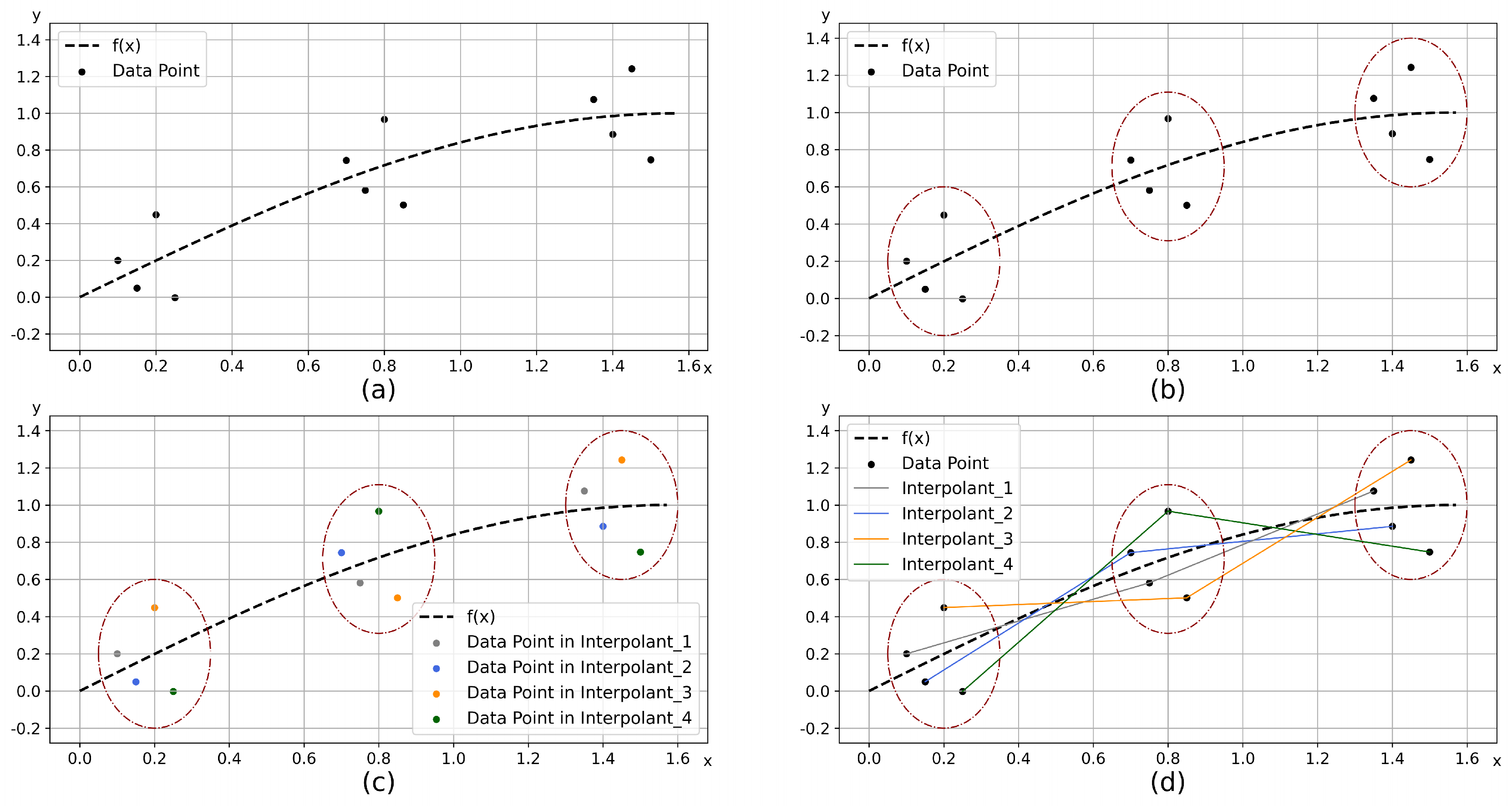
Figure 1. Overview of the proposed approach for ASISO. (a) The dataset contains multiple noisy samples, and the true functional relationship between x and y is f(·). (b) In the first step, we use the K-Space algorithm to perform unsupervised clustering on the dataset and divide the original feature space into several subspaces. (c) Interpolation matching of samples between adjacent subspaces is performed using the K-Match algorithm, and sample points with the same color belong to the same class to be interpolated. (d) Piecewise linear interpolation is performed on samples under different classes, and inserting equidistant sample points on lines of different colors in adjacent subspaces.

Figure 2. The synthetic data by ASISO. (a) The true relationship between x and y,

y = x^{3}

. The sample size is 200. (b) Adding Gaussian noise. (c) Let

k = 6, η = 100

, processing with ASISO, the sample size was increased to 3808.

Figure 2. The synthetic data by ASISO. (a) The true relationship between x and y,

y = x^{3}

. The sample size is 200. (b) Adding Gaussian noise. (c) Let

k = 6, η = 100

, processing with ASISO, the sample size was increased to 3808.

Figure 3. The synthetic data by ASISO. (a) The true relationship between x and y,

y = x^{3}

. The sample size is 200. (b) Adding Gaussian noise. (c) Let

k = 6, η = 100

, processing with ASISO, the sample size was increased to 3808.

Figure 3. The synthetic data by ASISO. (a) The true relationship between x and y,

y = x^{3}

. The sample size is 200. (b) Adding Gaussian noise. (c) Let

k = 6, η = 100

, processing with ASISO, the sample size was increased to 3808.

Figure 4. Changes in the MSE under different k values.

Figure 5. Changes in the MSE under different

η

values.

Figure 5. Changes in the MSE under different

η

values.

Figure 6. Changes in the

p (α)

under different

η

values.

Figure 6. Changes in the

p (α)

under different

η

values.

Figure 7. Comparison of MSE on artificial data sets.

Table 1. Artificial Data Sets.

Artificial Data Sets	$ϵ_{i}$ Distribution	Samples	$(P, P_{1}$ )
$D_{1}$	20%-N(0,64) 30%-U(-8,8) 50%-N(0,0.04)	500	(5,3)
$D_{2}$	20%-N(0,64) 30%-U(-8,8) 50%-N(0,0.04)	200	(5,3)
$D_{3}$	20%-N(0,64) 30%-U(-8,8) 50%-N(0,0.04)	1500	(5,3)
$D_{4}$	20%-N(0,64) 30%-U(-8,8) 50%-N(0,0.04)	500	(1,3)
$D_{5}$	20%-N(0,64) 30%-U(-8,8) 50%-N(0,0.04)	500	(20,10)
$D_{6}$	40%-N(0,64) 45%-U(-8,8) 15%-N(0,0.04)	500	(5,3)

Table 2. Experimental Results on Benchmark Data Sets.

Data sets	Processing	Hyperparameter	Testing MAE ( $10^{- 2}$ )
Data sets	Processing	Hyperparameter	KNN	RF	MLP	SVR	GBDT
Bike Sharing	-	-	$2.20$	$0.12$	$0.54$	$4.26$	$0.23$
	ASISO	$k = 150, η = 10$	$2.00$	$0.06$	$0.25$	$4.12$	$0.19$
Facebook	-	-	$6.60$	$2.25$	$8.19$	$7.34$	$1.33$
	ASISO	$k = 2, η = 10$	$6.41$	$1.59$	$2.02$	$7.36$	$1.12$
Air Quality	-	-	$2.99$	$2.57$	$4.80$	$3.87$	$2.58$
	ASISO	$k = 20, η = 100$	$2.89$	$2.55$	$2.08$	$3.84$	$2.77$
Forest Fires	-	-	$4.06$	$4.93$	$10.58$	$7.36$	$4.49$
	ASISO	$k = 10, η = 100$	$3.89$	$4.32$	$4.80$	$10.05$	$4.14$

Disclaimer/Publisher’s Note: The statements, opinions and data contained in all publications are solely those of the individual author(s) and contributor(s) and not of MDPI and/or the editor(s). MDPI and/or the editor(s) disclaim responsibility for any injury to people or property resulting from any ideas, methods, instructions or products referred to in the content.

© 2023 by the authors. Licensee MDPI, Basel, Switzerland. This article is an open access article distributed under the terms and conditions of the Creative Commons Attribution (CC BY) license (http://creativecommons.org/licenses/by/4.0/).

Copyright: This open access article is published under a Creative Commons CC BY 4.0 license, which permit the free download, distribution, and reuse, provided that the author and preprint are cited in any reuse.

MDPI Initiatives

Important Links

Choose an area of interest and we will send you notifications of new preprints at your preferred frequency.

Disclaimer

ASISO: A Robust and Stable Data Synthesis Method to Optimize Samples

Abstract

1. Introduction

2. Related Work

3. Proposed Method

3.1. Overview

3.2. K-Space

3.3. K-Match

3.4. Supplements

4. Experiments

4.1. Artificial Data Sets

4.1.1. Hyperparameter Selection

4.1.2. Comparison of Optimization Performance

4.2. Benchmark Data Sets

5. Conclusions

References

MDPI Initiatives

Important Links

Subscribe