Prediction of Reflection Seismic Low Frequency Components of Acoustic Impedance Using Deep Learning

The unreliable prediction of the low frequency components from inverted acoustic impedance causes uncertainty in quantitative seismic interpretation. To address this issue, we first calculate various seismic and geological attributes that contain low frequency information, such as relative geological age, interval velocity, and integrated instantaneous amplitude. Then, we develop a method to predict the low frequency content of seismic data using these attributes, their high frequency components, and recurrent neural networks. Next, we test how to predict the low frequency components using stacking velocity obtained from velocity analysis. Using all the attributes and seismic data, we propose a supervised deep learning method to predict the low frequency components of the inverted acoustic impedance. The results obtained in both synthetic and real data cases show that the proposed method can improve the prediction accuracy of the low frequency components of the inverted acoustic impedance, with the best improvement in a real data example of 57.7% compared with the impedance predicted using well log interpolation.

Keywords:

Subject: Environmental and Earth Sciences - Geophysics and Geology

1. Introduction

The low frequencies in inverted acoustic impedance (AI) profiles are crucial in quantitative seismic interpretation, since the impedance can be directly related to reservoir parameters such as porosity and water saturation.

One way to build the low frequency model is to extract the low frequencies from well logs (e.g., P-impedance, the product of the density and sonic logs), and interpolate the low frequencies from different wells laterally along interpreted horizons. Both the picked horizons and the interpolation can be incorrect. This can cause problems when the geological setting becomes complex, or if the number of wells is limited. For instance, the rock properties (e.g., velocity and density) can change abruptly laterally due to faulting or changes in the depositional environment. Another way of predicting the low frequency components of AI is based on L1-norm regularized sparse spike inversion [1,2,3,4,5,6]. These methods assume a sparse set of reflection coefficients. Therefore, we can make prediction of the reflectivity by adjusting the regularization parameter based on the L1 norm. However, we are still not able to fully recover the low frequency components due to the absence of the low frequencies in seismic data or low signal-noise-ratio (SNR), although this method may accurately predict the location of major reflection coefficients. Bianchin et al. [7] proposed a method to predict the broadband acoustic impedance using harmonic reconstruction and interval velocity, which improves the prediction accuracy of the low frequencies in the AI. However, one of the issues in this method is that the interval velocity derived from raw seismic data can be unreliable, and this will make the prediction unstable if the data quality is low.

Another family of low frequencies prediction is to predict the low frequencies of seismic data directly using their high frequencies in seismic data processing stage. For example, Wu et al. [8] and Hu and Wu [9] proposed direct envelope inversion to retrieve the low wavenumber components based on the instantaneous amplitude and phase of the seismic data. These authors demonstrated that this method could effectively recover the low wavenumber components, improving full waveform inversion (FWI) of the velocity model. Hu et al. [10] proposed a beat tone inversion to predict the low wavenumber components using the high frequency components of seismic data. The main idea in their work is that the interference between two signals with slightly different frequencies can be used to demodulate a low frequency signal using its envelope. Then they developed a deep transfer learning approach to predict the low frequency based on the beat tone concept [10]. Li and Demanet [11,12] proposed a phase and amplitude tracking method to extrapolate the low frequency components by decomposing seismic signals into atomic events, which then are parameterized by solving a nonconvex least-squares optimization problem. Sun and Demanet [13] use a deep learning method to directly predict the low frequencies of the raw band-limited shot records using their high frequency components (e.g., 5.0-20.0 Hz). These works show promise in estimating the low frequencies of seismic data directly using their high frequency components. In this paper, we use the high frequencies of seismic data to predict their low frequencies using recurrent neural networks (RNNs), which helps to improve the prediction accuracy of AI inversion. Due to the success of the application of deep learning methods in many different fields [14,15,16,17,18,19,20], deep learning methods have gained attention in geophysics, both in the industry and academia [10, 21, 22]. The inverse problems in geophysics are like problems in many other fields, such as face recognition, natural language processing, and self-driving cars and involve building a predictive model to predict the future using preexisting data. Hampson et al. [23] proposed using a probabilistic neural network (PNN) to predict well logs directly using seismic attributes. Li and Castagna [24] used the support vector machine (SVM) to classify seismic attributes. Saggaf et al. [25] investigated how to classify and identify reservoir facies from seismic data using a competitive neural network.

Recently, convolutional neural networks (CNN) and recurrent neural networks (RNN) have been successfully applied in many fields [26,27,28]. These methods have been used on seismic data for a variety of tasks such as fault detection and facies classification [29,30,31,32]. Das et al. [21] predicted acoustic impedance and petrophysical properties using CNNs. Alfarraj and AlRegib [33] proposed a semi-supervised sequence model to estimate the elastic impedance from prestack seismic data.

Prediction of the low frequency component for inverted acoustic impedance remains challenging. In this paper, we attempt to address this challenge using seismic attributes that may contain low frequency information. These include the relative geological age attribute and the apparent time thickness attribute. We introduce a deep learning architecture and demonstrate how to predict the low frequencies of AI using various combinations of attributes and methods, first using synthetic seismic data. Finally, we apply the proposed methods to field seismic data from the Midland basin and evaluate the result.

The objective of this paper is to predict, and substitute for, the missing low frequency content of the seismic data without the use of well logs or possibly incorrect seismic interpretations of, for example, lithology or mineralogy away from well control. Although we have mineralogy information from the interpretation of the well log curves, such as the volumetric percentage of quartz and limestone, we do not directly use this information to predict the low frequencies between wells because we do not have accurate mineralogy information away from wells. On the other hand, we do not use mineralogy as our output because the relationship between seismic data and mineralogy is highly nonunique and underdetermined, and thus beyond the scope of this work.

2. Workflow and Method

We assume in this section that the seismic signal s(t) can be represented as the convolution of a wavelet w(t) and reflectivity r(t) plus random noise δ(t):

s (t) = w (t) * r (t) + δ (t),

(1)

where the reflectivity is defined by

r (t) = \frac{I_{p} (t) - I_{p} (t - 1)}{I_{p} (t) + I_{p} (t - 1)},

(2)

where I_p is the AI at time t. Seismic processing attempts to create this ideal model on the seismic data, but this goal is often not achieved due to problems like multiples and incorrect scaling. Furthermore, the temporal and spatial variation of the seismic wavelet is only approximately known, even at well locations,

One of the main goals of seismic inversion is to invert equations (1) and (2) to predict the acoustic impedance using seismic data using various inversion techniques. In conventional seismic inversion [5,6], we first need to extract a wavelet using seismic and well log data, then construct the objective function based on the physical relationship between the wavelet and seismic data. We can invert the seismic data to AI using a variety of optimization methods [1,3,4].

In contrast, machine/deep learning algorithms try to build the linear/non-linear mapping function between the target inversion parameters and seismic data by training a model using feature-label data, where the “feature” and “label” refer to the seismic data and target inversion parameters, respectively [34].

Potential issues for the conventional inversion methods include: 1) uncertainties caused by inaccurate wavelets; and 2) the oversimplified physics of the forward model in equation (1). Since the learning-based inversion methods do not require extracting wavelets or making physical assumptions they offer an alternative approach that may have advantages in certain cases. However, learning-based inversion methods have a high requirement for training data quantity and quality, which might not be met easily in a real case. This can result in poor generalization for predicting new data. The question remains: Can such methods outperform physics-based methods in predicting absolute acoustic impedance?

2.1. Convolutional Neural Networks

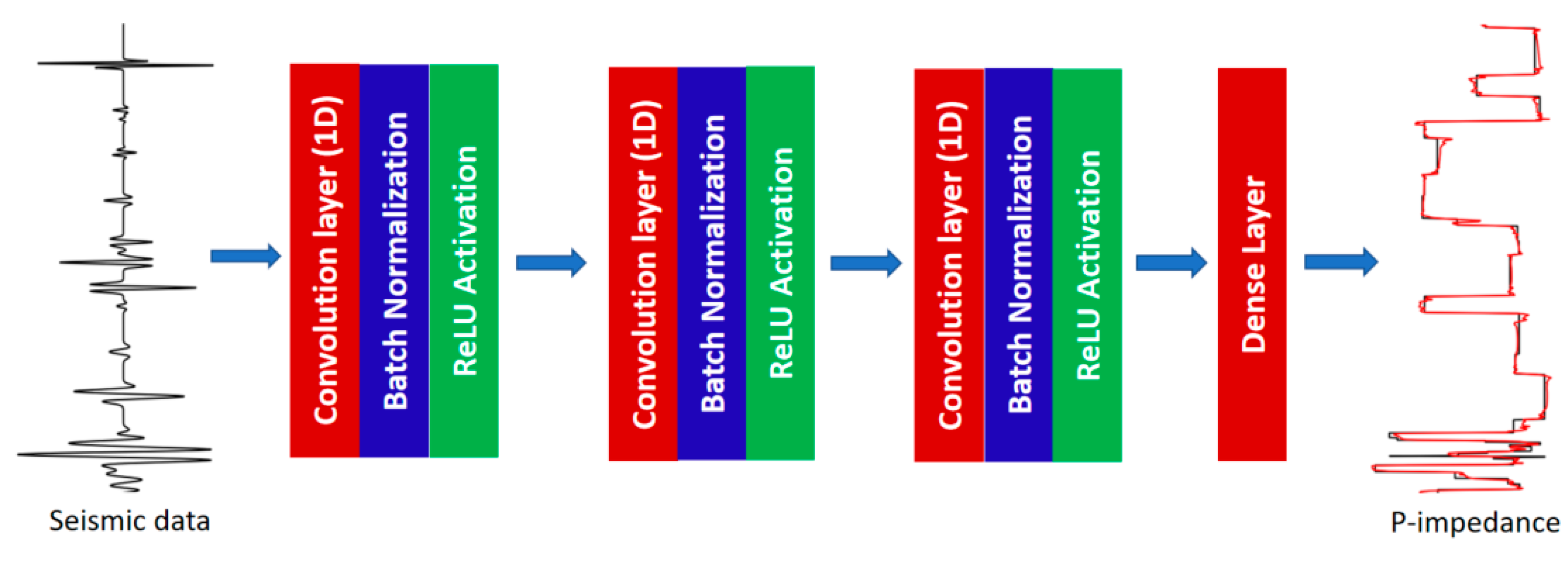
Convolutional neural networks (CNNs) have achieved success in many kinds of applications [15,16,18], so we will apply this method here. The CNN architecture we used contains three convolution layers at the beginning and one dense layer at the end of this network (see Figure 1). Each convolution layer is followed by batch normalization and a ReLU activation function. The batch normalization helps reduce the covariate shift and smooths the objective function, which improves the model performance. The ReLU activation function enhances the learning of a non-linear relationship and has been shown to improve the performance over the sigmoidal functions used in older networks. The inputs in our case are poststack seismic data and attributes after being properly processed, and the target log is the AI or reflectivity. Note that the poststack seismic data contain AVO effects, which could decrease the prediction accuracy of rock properties, here calculated assuming normal incidence. With sufficient training data, neural network could learn the proper relationship between stacked amplitude and acoustic impedance, in the presence of such AVO effects. A better approach would be to use the pre-stack data or pseudo-P and S sections derived from the pre-stack data, but we restrict the problem to normal incidence in this study.

The hyperparameters in this network include the channel, kernel size, and learning rate, which need to be set case by case. Since the theory of deep learning offers insufficient prior insight, the number of convolutional layers used in a real work needs to be tested for each situation.

2.2. Recurrent Neural Networks

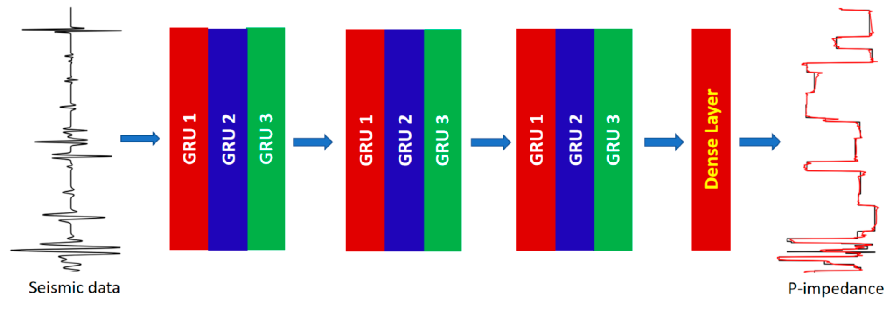
Recurrent neural networks (RNNs) are deep learning methods which have been successfully applied to process time series data [14,35]. In this work, we used three bidirectional gated recurrent units (GRUs) stacked layers and one dense layer at the end of this network. Each stacked layer has three stacked GRUs. The input in our case is poststack seismic data after being properly processed, and the target log is the AI or reflectivity. The number of stacked layers and the number of single GRUs are subject to change in each case. The hyperparameters in this network include the hidden layer size and learning rate, which need to be tested.

Figure 2. Architecture of RNNs.

3. Results

3.1. Synthetic data test

3.1.1. Synthetic data test based on rock physics modeling

The first synthetic data we use to test the proposed methods is produced using rock physics modeling (RPM) and a convolutional model. The data is purely synthetic data, and there is no added noise in this dataset. Therefore, we can use this dataset to evaluate how well each machine learning model performs with perfect data.

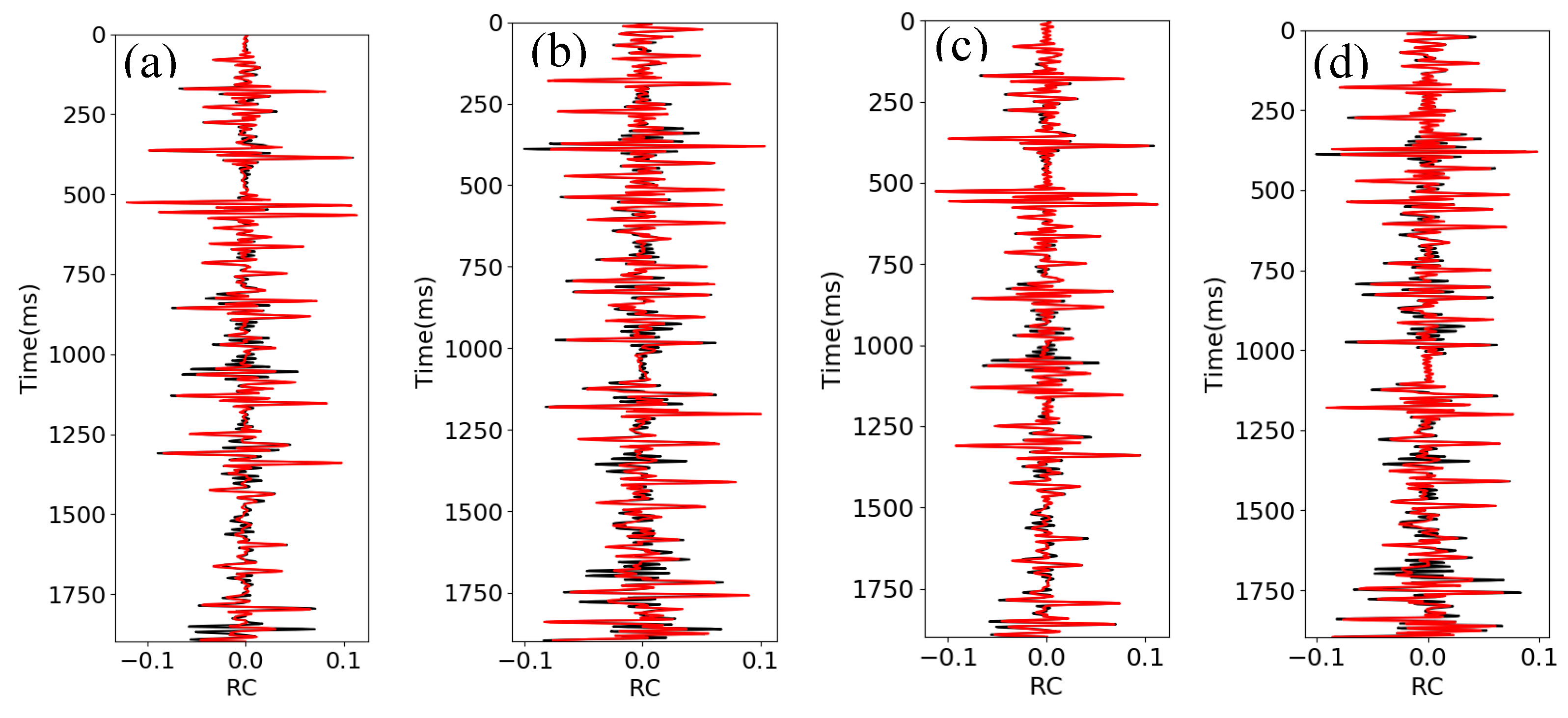
We use 20 pseudo wells to train the predictive model, five wells for validation, and five wells for the blind test. Figure 3 shows the reflectivity predicted from the seismic data using the CNN and RNN methods. The black curve shows the true reflectivity, and the red curve shows the predicted reflectivity. The input we use in this example is original synthetic seismic data (seismic amplitudes, not attributes). As seen in this figure, both CNN and RNN successfully predict the reflectivity with high accuracy, with an R² score of about 0.86 from the CNN and 0.87 from the RNN, and a correlation coefficient (CC) of 0.93 from the CNN and RNN for the blind test. Therefore, both the CNN and RNN algorithms successfully map the physical relationship between seismic data and reflectivity.

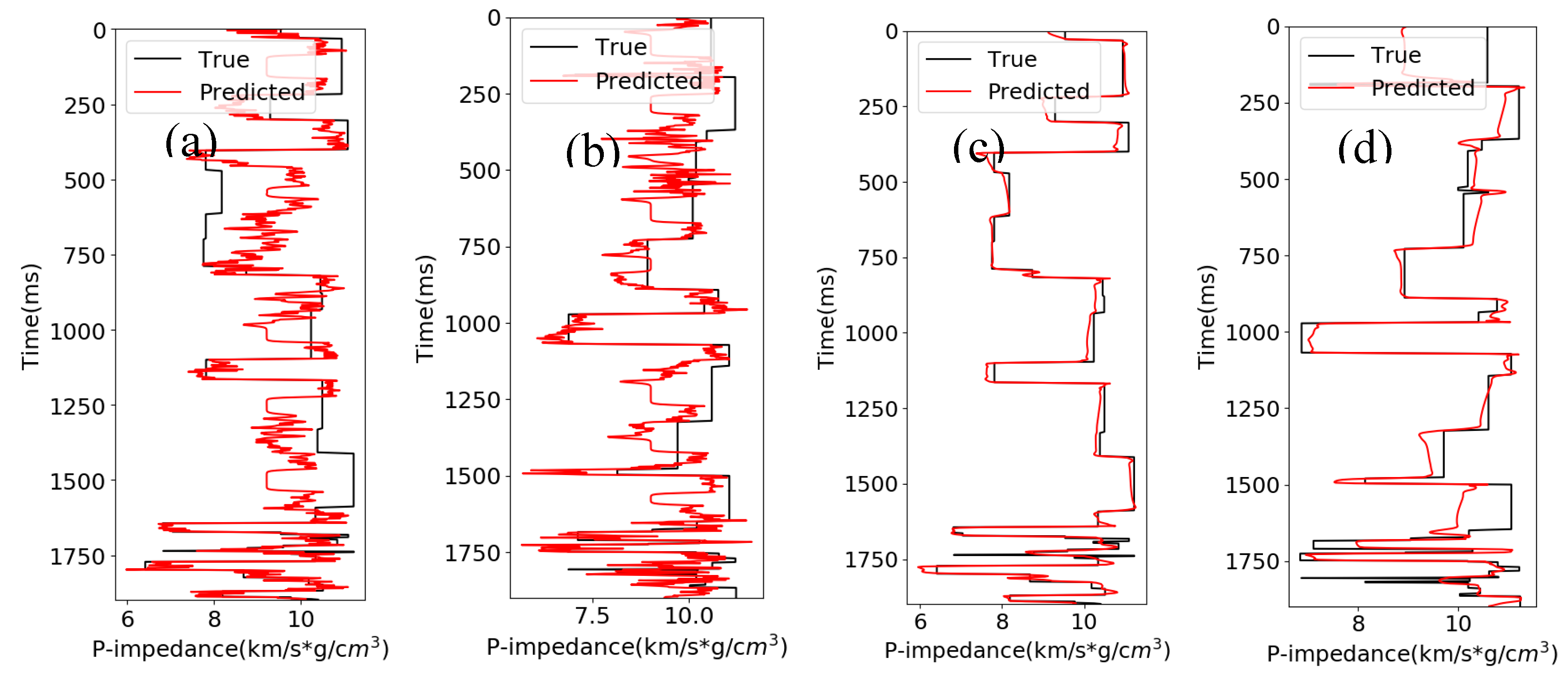
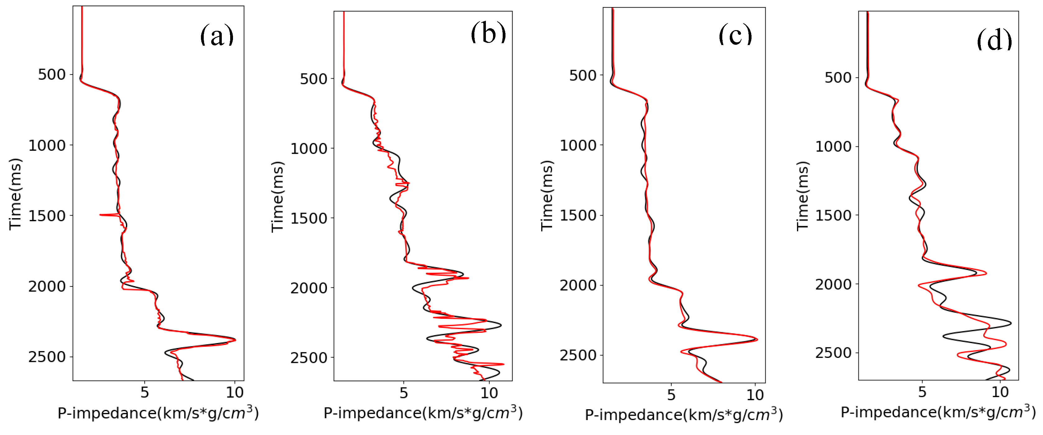
We then use the same synthetic data to test if we can predict the AI using the reflectivity. Figure 4 is the predicted AI from reflectivity using the CNN and RNN algorithms. The black curve in Figures is the true AI, and the red curve is the predicted AI. The results show that the CNN does not predict well in this case, with an R² score of 0.34 and a CC of 0.70 for the blind test. In comparison, the results from RNN show that it performs well in this task, with an R² score of 0.95 and a CC of 0.98 for the blind test.

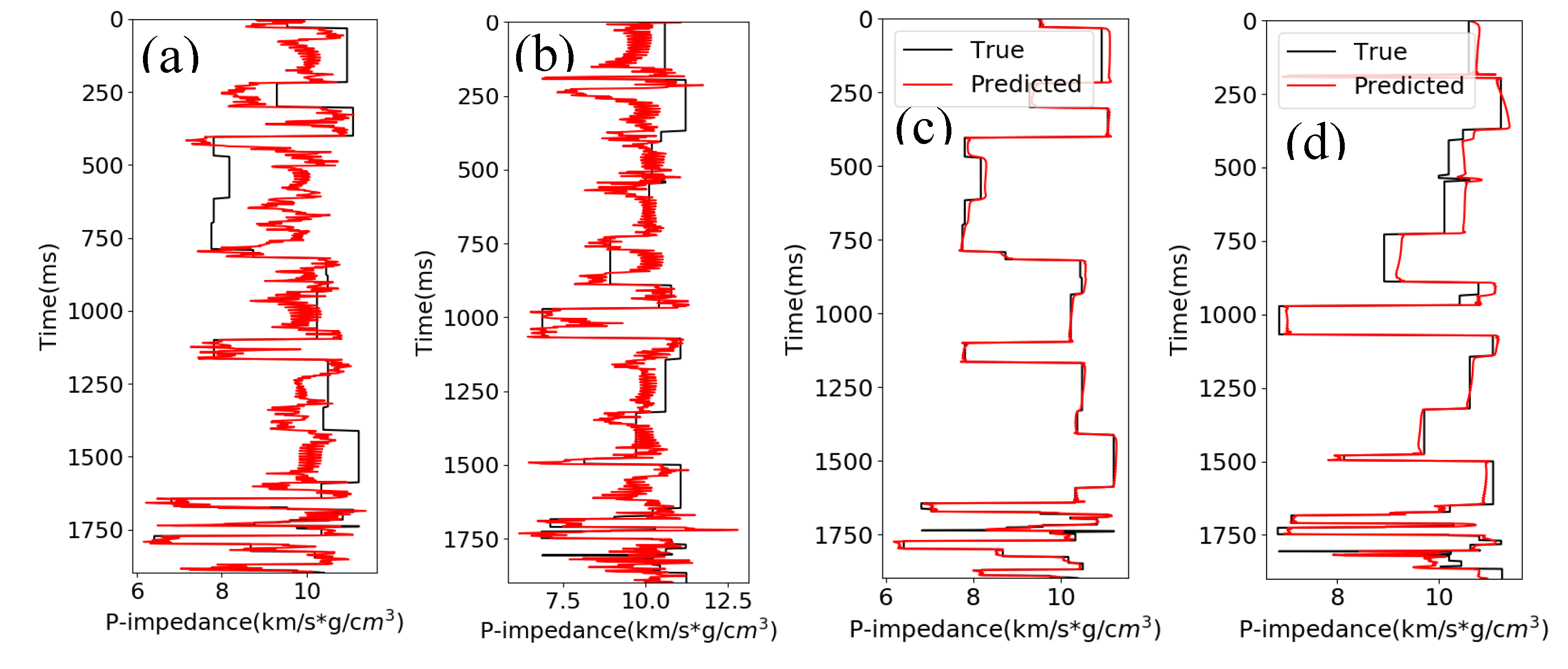
We then predict the AI directly using seismic data as input. Figure 5 shows the predicted AI from seismic data using the same CNN and RNN approaches used in the last section. The results show that the CNN gives a poor predication of the AI well in this case, with an R² score of 0.20 and CC of 0.77 for the blind test. In contrast, the results from RNN show that it performs well in this task, with an R² score of 0.67 and CC of 0.85 for the blind test.

From these three tests, we find that: 1) the RNN is suitable for all three tasks, but the performance deteriorates when it comes to predicting the AI using seismic data directly; 2) the CNN architecture used here is suitable for predicting the reflectivity from seismic data, but not for predicting the AI using either reflectivity or seismic data.

3.1.2. Marmousi model 2 test

To further test how well the proposed methods work, we used the Marmousi model 2 [36]. This model is an extension of the original acoustic Marmousi model created by the Institute Français du Pétrole (IFP) [37], which has the same structure and velocity as Marmousi model 2, but the model size of Marmousi model 2 is wider and deeper and it is fully elastic [36]. Marmousi model 2 is 17.0 km in width and 3.5 km in depth. More details about this model are given in Martin [36]. The model has velocity and density volumes only in the depth domain, so we convert them into the time domain with a time interval of 4.0 ms using the true velocity model. We also reduced the size of the model to a maximum time of 2700.0 ms and a CDP number range of 400 to 2350. We create synthetic seismic data using a 30 Hz Ricker wavelet based on a convolution model to test the proposed methods. Figure 6a is the AI, and Figure 6b is the poststack seismic data after prestack time migration (PSTM) processing.

3.1.3. Low frequency attributes

The geological age of a formation at a given location is associated with the depositional environment and various rock properties, such as velocity, density, and porosity. The geological age can therefore contribute to the prediction of the low frequency components of AI. We first choose the horizons and faults from the Marmousi model 2 (see Figure 7a). Then, we use these faults and horizons to construct the relative geological age attribute as an index with different values for each formation (see Figure 7b). The index is approximately proportional to geologic age, but not exactly since it ignores the fluctuation in sedimentation rate and erosion.

The rock properties are not just controlled by geological age but also governed by burial depth. For instance, rocks deposited at the same geological time but buried in different depths can have different velocities. Therefore, one can use depth to constrain the prediction of the low frequencies in AI. We use the time-depth relationship along the horizons at pseudo well locations to convert the time to depth. Then, we interpolate the depth vertically to obtain the depth volume. The depth volume here is an attribute that we use to calculate the interval velocity. It is calculated using very limited information (e.g., 5 or 10 pseudo wells). Compared with the true depth and the predicted depth in Figure 8, we find that they give a good match, which means that we can predict the depth attribute using this method accurately. Note that there are some mismatches at around CDP of 1500. This is because of the complexity of the geological structure near this location, which means that the velocity changes rapidly both horizontally and vertically. Since the method we used to calculate the depth attribute uses only a few pseudo wells and horizons, it fails to capture these velocity variations.

With the depth information at each time location, we can then calculate the interval velocity. Figure 9a is the true interval velocity, and Figure 9b is the interval velocity calculated using the depth attribute we create in Figure 8b. Although the details between these two figures are different, the velocity structure looks similar, which means that the interval velocity we create can provide low frequency information. Note that we only use four horizons in our example. Increasing the number of horizons to calculate the interval velocity would improve the vertical resolution and the prediction of low frequencies.

Instantaneous amplitude has been used to recover the ultra-low frequencies of the seismic signal (i.e., frequencies below the lowest frequency in the source spectrum) Wu et al. [8] proposed an envelope inversion method using a nonlinear seismic signal model to recover the low frequencies using instantaneous amplitude. This is based on an empirical relationship between the instantaneous envelope and the low frequencies at a given locality.

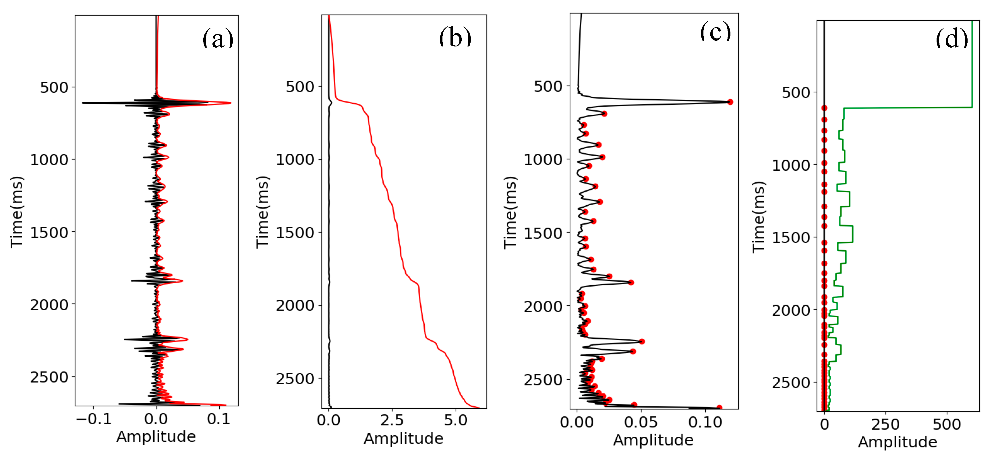
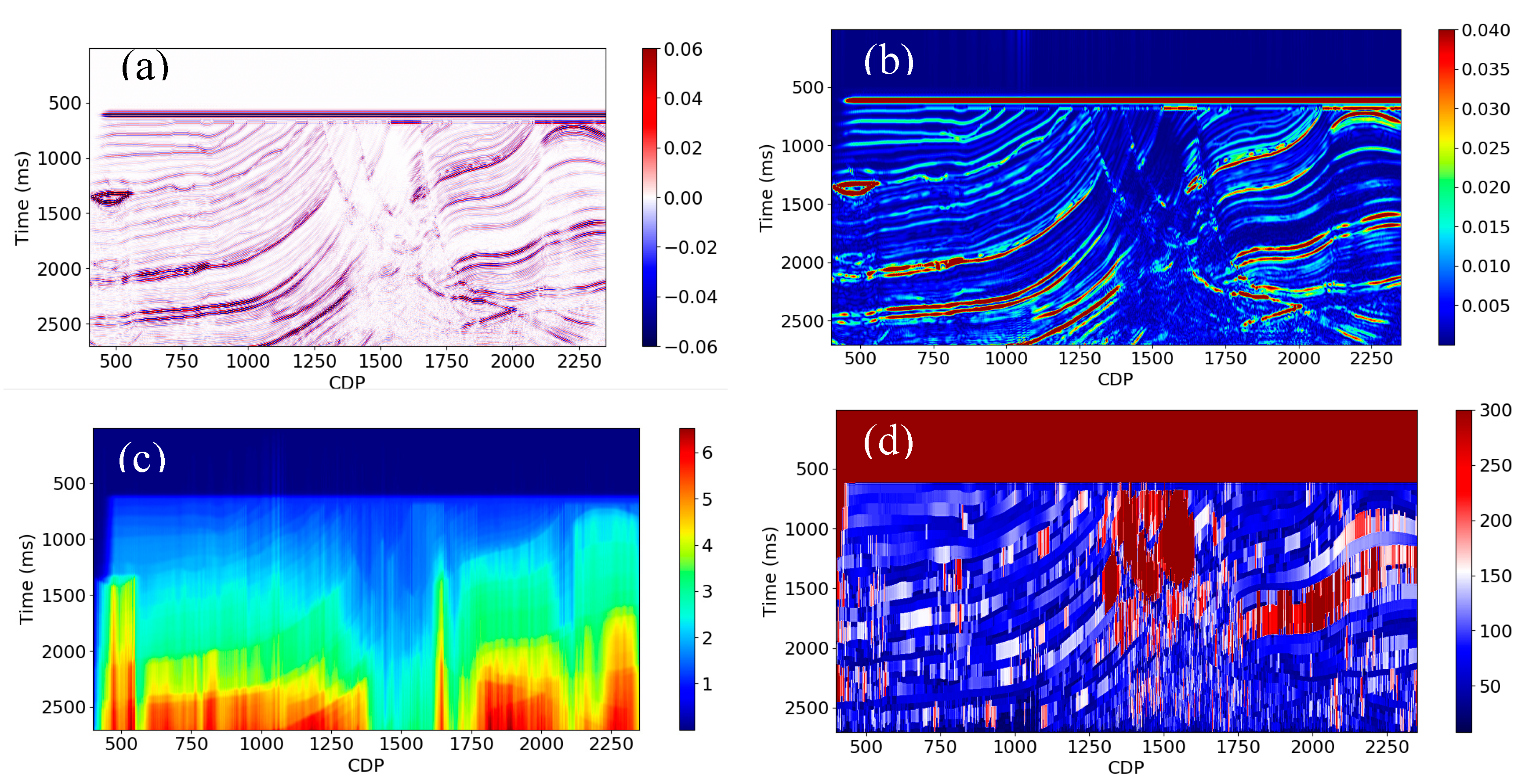
In contrast, we use instantaneous amplitude as one input for deep learning models and let the model learn the relationship. We also produce two more attributes (Figure 10) using the instantaneous amplitude: integrated instantaneous amplitude and apparent time thickness (time thickness between adjacent peaks on the instantaneous amplitude curve). Figure 11 are the 2D sections for each of the attributes showing the apparent geological structures, which could in turn be related to the low frequencies. Together these attributes make a positive contribution to predicting the low frequencies of AI, although it is difficult to evaluate them separately.

3.1.4. Predicting the low frequency components of seismic data

Seismic data often lacks frequencies below 5.0 Hz and this limits our ability to invert seismic data for absolute rock properties. This section shows how we predict the low frequency components of seismic data using higher frequencies that are present (e.g., 10.0-40.0 Hz).

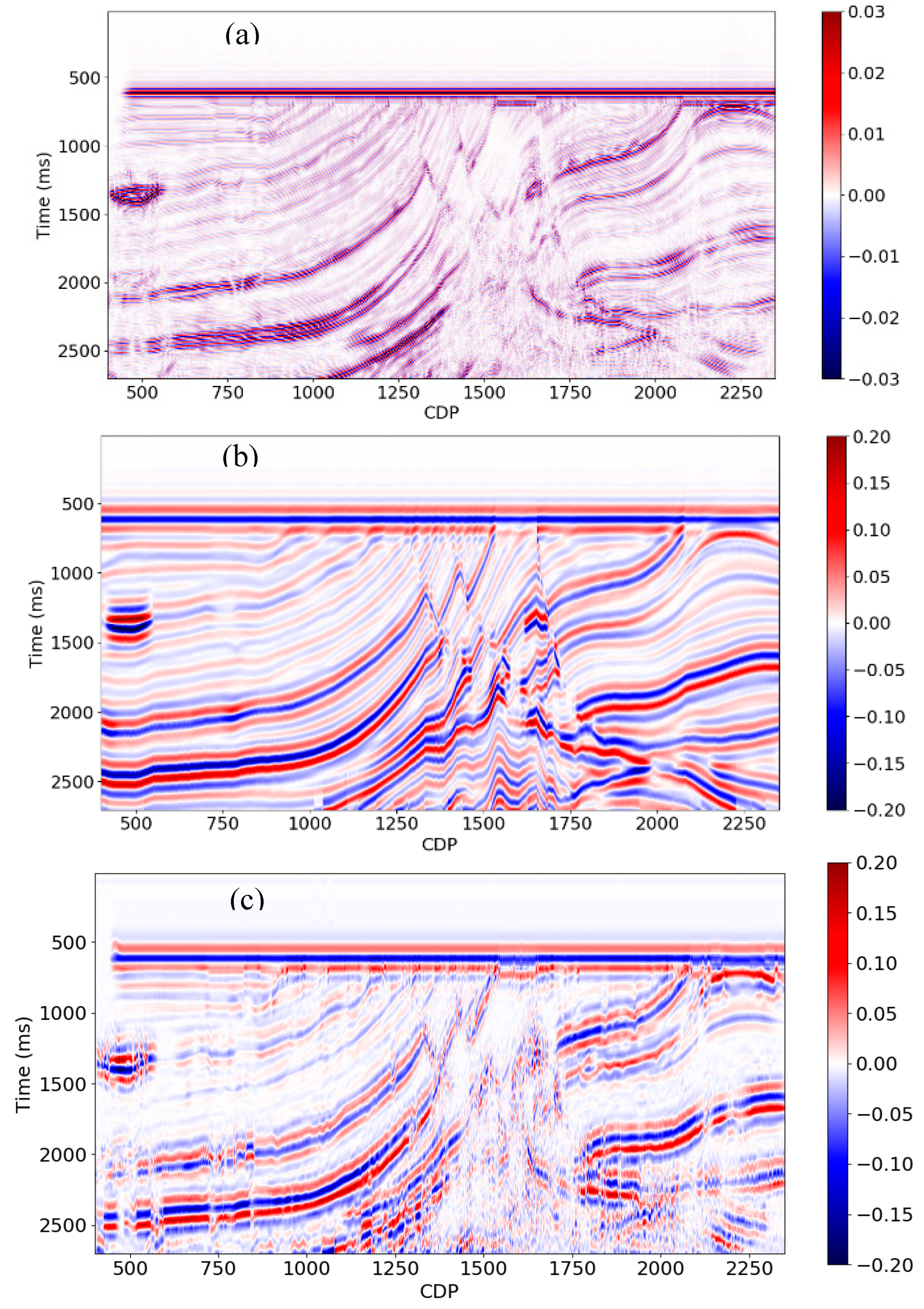
We will use the Marmousi model for illustration. Figure 12a shows the simulated PSTM data with a 5 - 40 Hz pass band. We create 0 - 5 Hz synthetic seismic using convolution model using a 0 -1 - 4 - 5 Hz bandpass filter (see Figure 12b). This is the low frequency model we wish to recover from the simulated PSTM data. Next, we choose 10 traces of data from the 5.0 - 40.0 Hz PSTM seismic data (Figure 12a) and 0.0 - 5.0 Hz synthetic seismic data (Figure 12b) as the training set. Finally, we predict the whole section using the model we trained with these 10 traces. We tested various CNN and RNN architectures and found that the RNN achieved better performance.

The results from the RNN are demonstrated in Figure 12c. The seismic section (including predicted low frequencies) in Figure 12c looks promising by comparing it with the seismic section (including true low frequencies) in Figure 12b. Figure 13 are the training and blind test results taken from the 2D line, with CDP = 2000 and 900, respectively. The black curve is the true synthetic seismic data (0-5.0 Hz), and the red curve is the predicted one. It shows that the R² score and CC are 0.92 and 0.96 for training results and 0.74 and 0.86 for blind test results. Considering the original PSTM seismic data is noisy, the prediction accuracy is acceptable. However, as seen in Figure 12c, the results are unstable and produce non-geological variations.

3.1.5. Predicting the low frequencies of AI

With all the attributes we created in addition to the conventional seismic attributes, we can test how each method works using different combinations of seismic attributes as input, on the 5-40 Hz Marmousi simulated PSTM.

We first compute a range of conventional seismic attributes. Then, we apply the stepwise regression method to optimize both the conventional attributes and the attributes proposed in this paper. In this method, we first select the attribute that has the strongest correlation with the AI; then we select the second attribute from the remaining attributes list that best fit the regression model with the AI by combining the first attribute selected in the previous step; we keep adding the remaining attributes to the regression model until the model performance improvement cannot meet the criteria we set beforehand; at last we check the model performance using validation dataset to ensure there is no overfitting. Finally, we obtain the following 11 best attributes:

▪: Depth attribute
▪: Interval velocity
▪: Average frequency
▪: Time
▪: Instantaneous amplitude
▪: Apparent polarity
▪: Apparent time thickness
▪: Amplitude weighted frequency
▪: Integrated instantaneous amplitude
▪: Relative geological age
▪: Filter 5/10-15/20

The additional attributes we created are on this list, so they are helpful to improve the prediction of the low frequencies. We then use these optimized attributes to test different methods with the same 10 traces for training. In this paper, we compared the RNN to two of most common algorithms. One is the Probabilistic Neural Network (PNN) [23], and the other one is multi-linear regression of the attributes. The PNN is trained by minimizing the validation error for each training data point by searching the optimal smoothing parameters sigma (σ). The new target log is then computed by combining the distance of the training and target log attributes and the target logs of the training set (see more details in [23]). 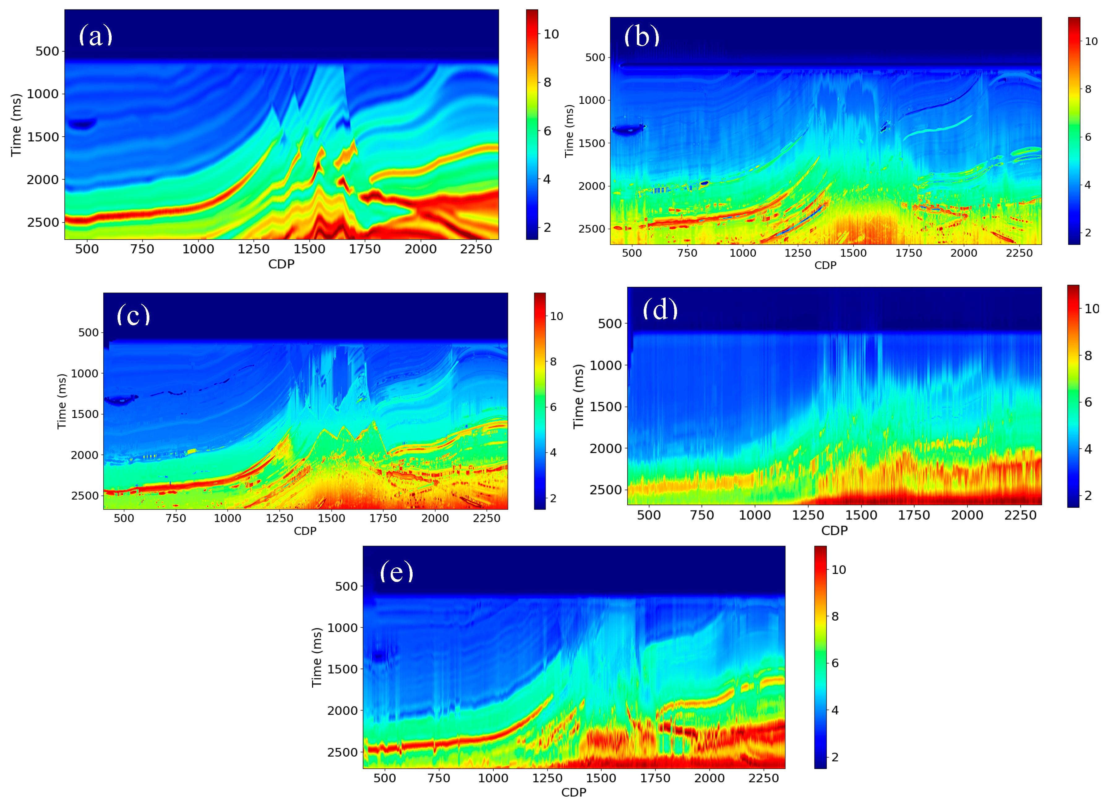Figure 14 (a) and (b) are the 0.0-5.0 Hz AI predicted using the new and conventional seismic attributes using PNN. Figure 15 (c) and (d) are the AI (0.0-5.0 Hz) predicted using the predicted low frequency seismic data and new attributes using RNN. The results from PNN show that the R² score and CC are 0.99 and 1.0 for training, and 0.95 and 0.98 for the blind test. The results from RNN show that the R² score and CC are 0.99 and 1.0 for training, and 0.95 and 0.97 for the blind test, respectively. As observed from Figure 14b, the blind test results from PNN have more high frequency noise than the blind test in Figure 14d from RNN, although the prediction accuracy is close. Figure 15 shows the results predicted using a different combination of attributes and methods, which reveals that the result predicted using the predicted low frequency seismic data and the new attributes produced in this work using RNN is the best. However, the performance could be different in different parts of this 2D section for different methods. For example, the results predicted from the new attributes and conventional attributes using PNN at around CDP of 500 are better than the results in Figure 15e at the same location, although the overall prediction accuracy from this result is better than the result from Figure 15b.

Table 1 is the validation summary for the AI (0.0-5.0 Hz) predicted from various combinations of attributes and methods. The R² score and CC in this table are the average value calculated using the entire 2D line. In comparison, the AI (0.0-5.0 Hz) predicted from the conventional attributes using PNN has the lowest prediction accuracy, with an average R² score of 0.84 and CC of 0.94. The result predicted from the proposed new attributes and RNN method achieves the highest prediction accuracy, with an average R² score of 0.93 and CC of 0.97. The improvement is 10.7% for the R² score.

Table 2 shows that the predicted low frequency components of AI improve the prediction accuracy of the absolute AI, with an improvement of 11.0%, which indicates that the low frequency components are critical in the AI inversion. RNN shows some benefit over PNN, and the new calculated attributes make a major contribution to the overall improvement in the prediction of low frequencies in this example.

3.1.6. Predicting the low frequencies using RMS velocity

Another important low frequency source is from the travel time information at different offsets recorded in seismic data. Bianchin et al. [38] discussed how to improve AI estimation using interval velocity calculated from tomography based on autoregressive models. In contrast, we attempt to directly predict the low frequencies of AI using deep neural networks from the RMS stacking velocity obtained from velocity analysis on common-midpoint (CMP) gathers containing nonzero offset recordings.

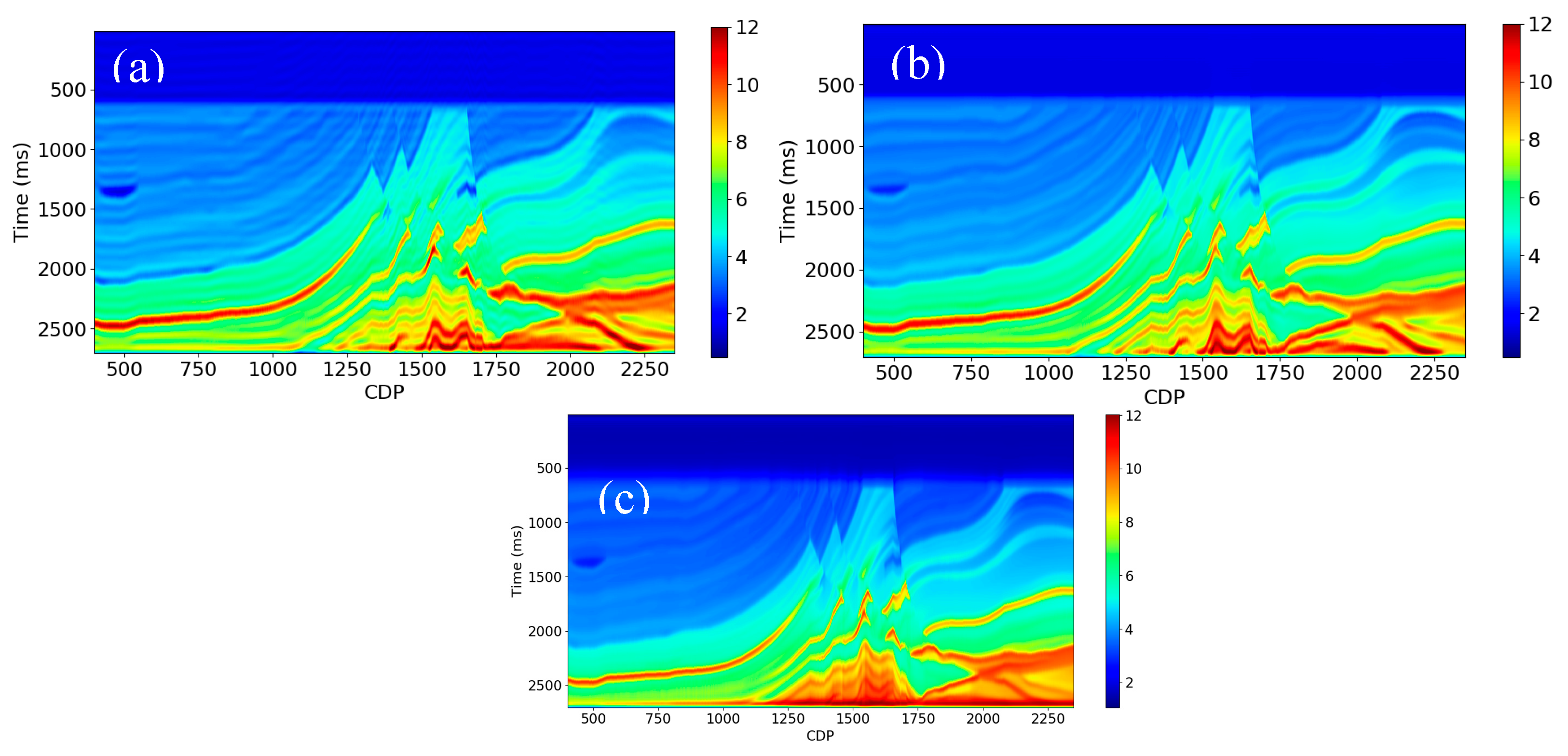
The Marmousi interval and RMS velocities are shown in Figure 16. We chose 10 traces of these data as the training set and trained a predictive model using RNN. Finally, we predicted the whole AI volume from the RMS velocity volume using this predictive model. The result is displayed in Figure 17b. As one can see in this figure, the predicted AI (0.0-5.0 Hz) is very close to the true AI (0.0-5.0 Hz) in Figure 17a, with an R² score of 0.98 and CC of 0.99. We then try to predict the AI (0.0-10.0 Hz) using the RMS velocity using the same workflow, and the results indicate that the prediction accuracy is decreased (see Figure 18). Next, we add the PSTM seismic data as an input in the training, and the prediction result is displayed in Figure 19b, which shows that the true and predicted AI (0.0-10.0 Hz) match each other very well, with an R² score of 0.98 and CC of 0.99. Finally, we try to predict the AI (0.0-10.0 Hz) from the RMS velocity and PSTM seismic data using RNN using only five pseudo wells. The result in Figure 19c closely matches the true AI (0.0-10.0 Hz), with an R² score of 0.97 and CC of 0.99, although it is not as good as the result predicted using 10 pseudo wells in Figure 19b. It reveals that the proposed method is not sensitive to the number of traces in the training set for this synthetic example.

Although we can theoretically predict the low frequencies accurately using the RMS velocity, there can be problems in a real case. First, the field data could be very noisy, which could cause many errors in the picking of the RMS stack velocity. Second, even a small, localized mis-picking can lead to a physically implausible interval velocity value [39]. Third, the static error from the inaccurate near-surface velocity could also cause an error in the picking of the RMS stack velocity. Fourth, the multiples in the raw seismic data can cause picking errors. Therefore, we need to be cautious in using the RMS stack velocity as an input to predict the low frequency components of AI.

3.2. Real data example

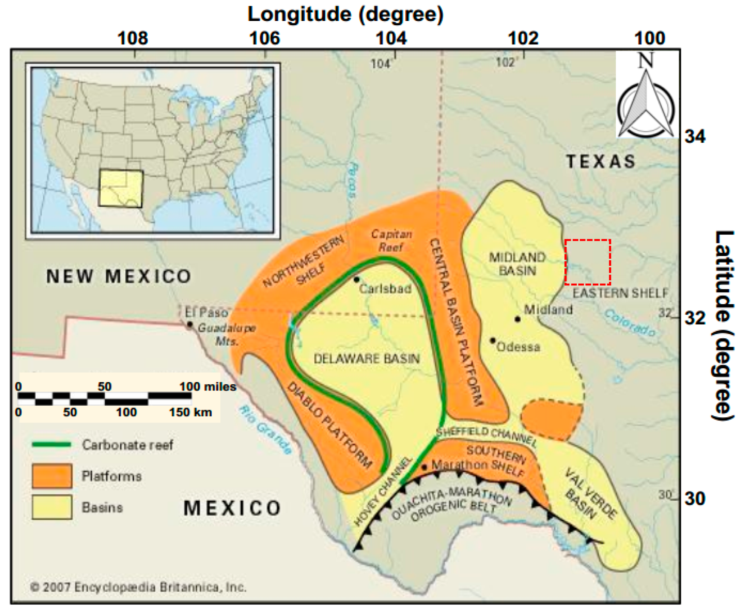
Next, we apply our techniques to a dataset from the Midland basin, which is an eastern sub-basin of the Permian basin, one of the largest Hercynian (Middle Devonian-Middle Triassic) structural basins in North America (Figure 20). Due to intense structural deformation and orogenic movement, the depositional environment of Midland basin is very complex from late Mississippian to early Permian time [40]. The sediments include coarse clastic sediments deposited near the basin shorelines, limestone, and extensive reef developed toward the ocean.

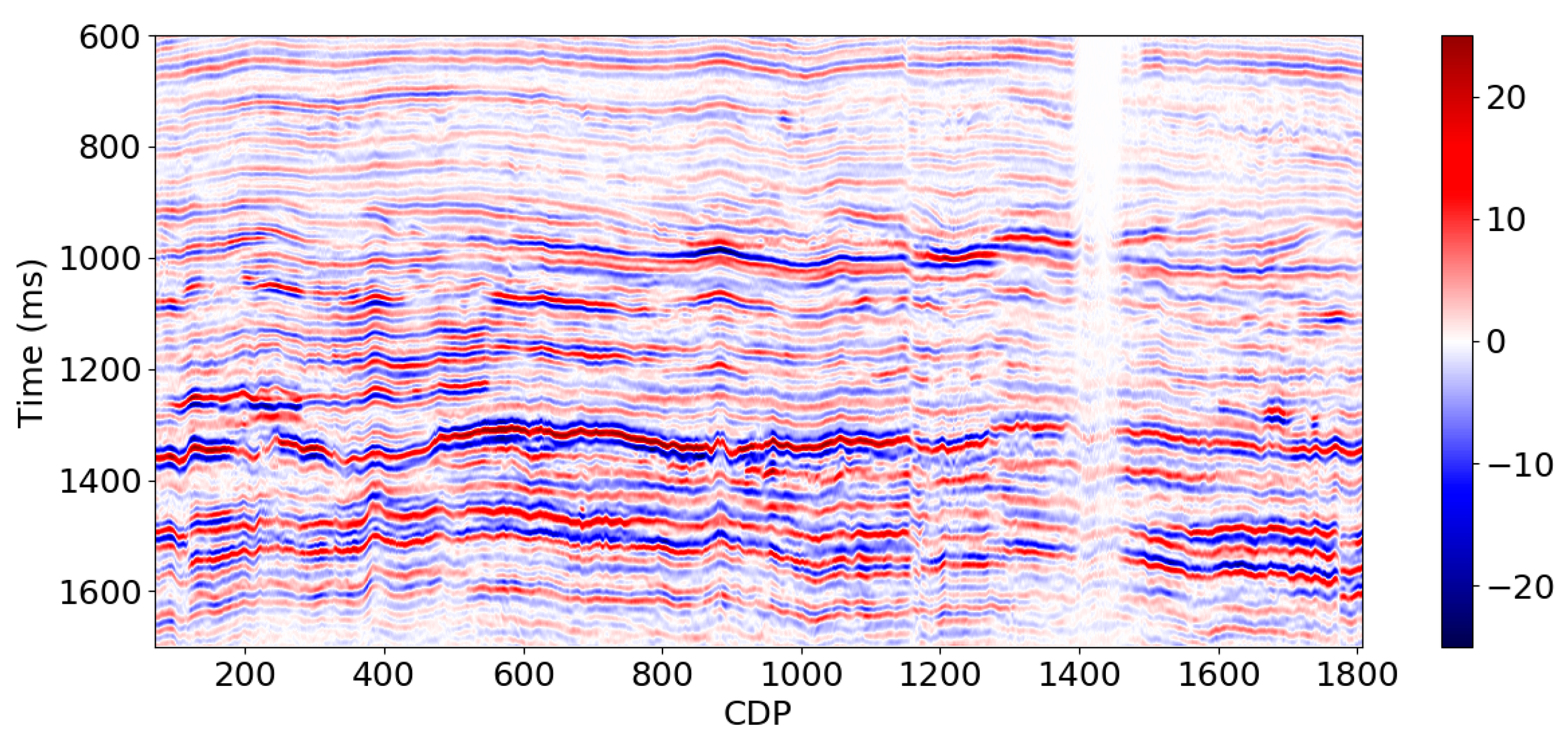
The target formations of interest in the field studied include Wolfcamp, Dean, and Spraberry with depths varying from 6000 to 8000 ft (1.0 to 1.5 s two-way seismic travel time). The lithology includes sandstone, shale, limestone, and dolomite, and shows dramatic lateral changes, making the AI prediction very difficult. The 3D seismic data for the study area covers approximately 50.0 mile². The sample interval is 2.0 ms, and the central frequency is approximately 50.0 Hz. The data contains prestack CDP gather and poststack PSTM seismic data (see Figure 21). In general, the seismic data quality is good. There are nine wells with high-quality logs in this area, and they are well-documented and edited. The log curves include density (RHOB) P-wave slowness (DT), S-wave slowness (DTS), and neutron porosity. The RMS velocity is stacking velocity picked manually by experienced seismic processing engineers.

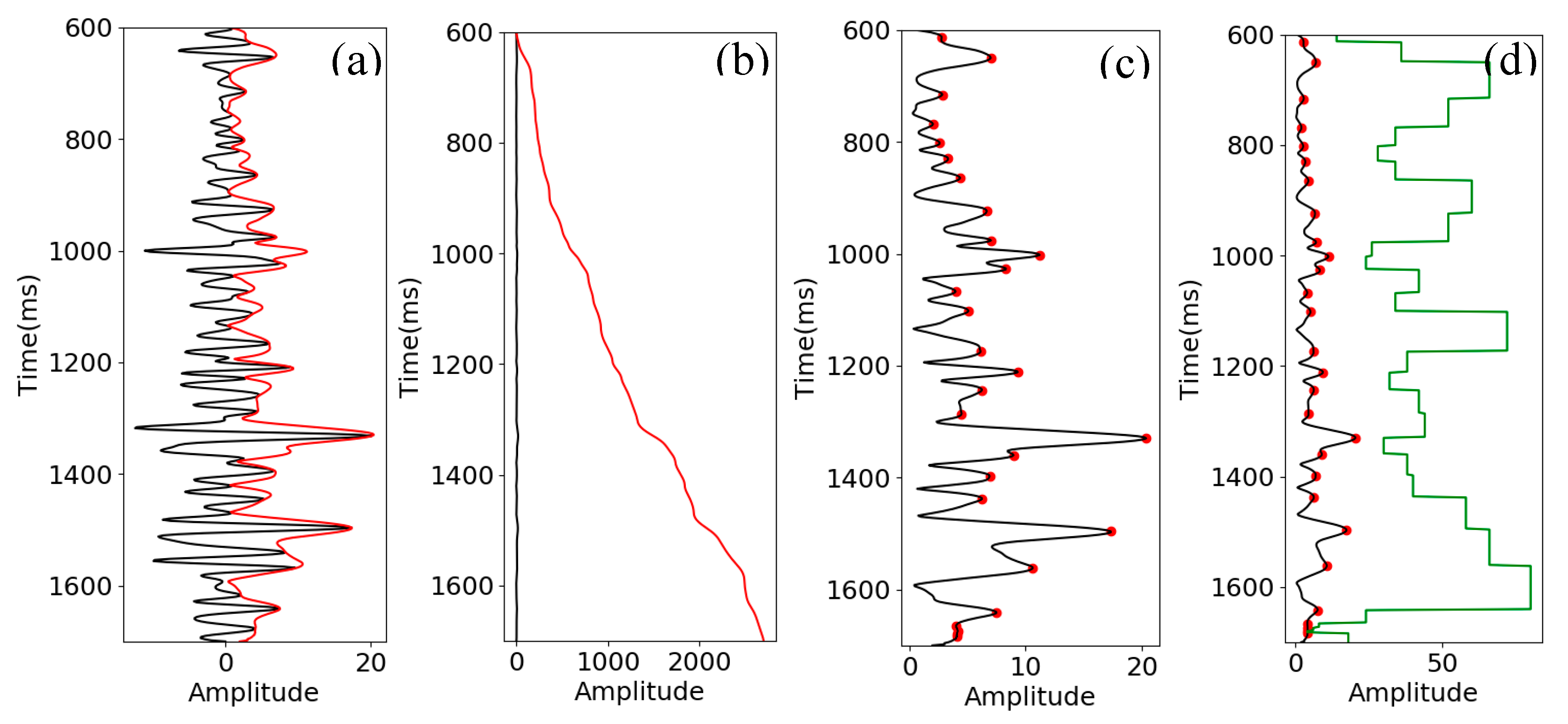
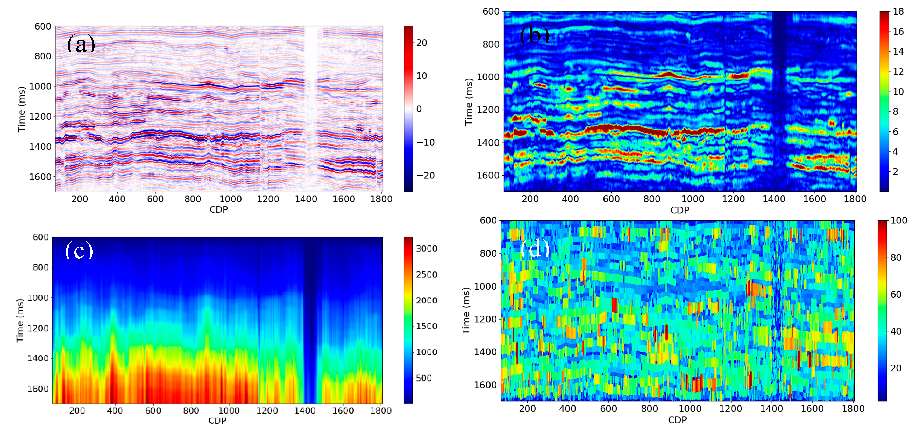
We created the relative geological age, instantaneous amplitude, integrated instantaneous amplitude, and apparent time thickness attributes from the PSTM seismic data using the same procedure described above (see Figure 22, Figure 23 and Figure 24). We did not produce the depth and interval velocity attributes due to the flat horizons in this area.

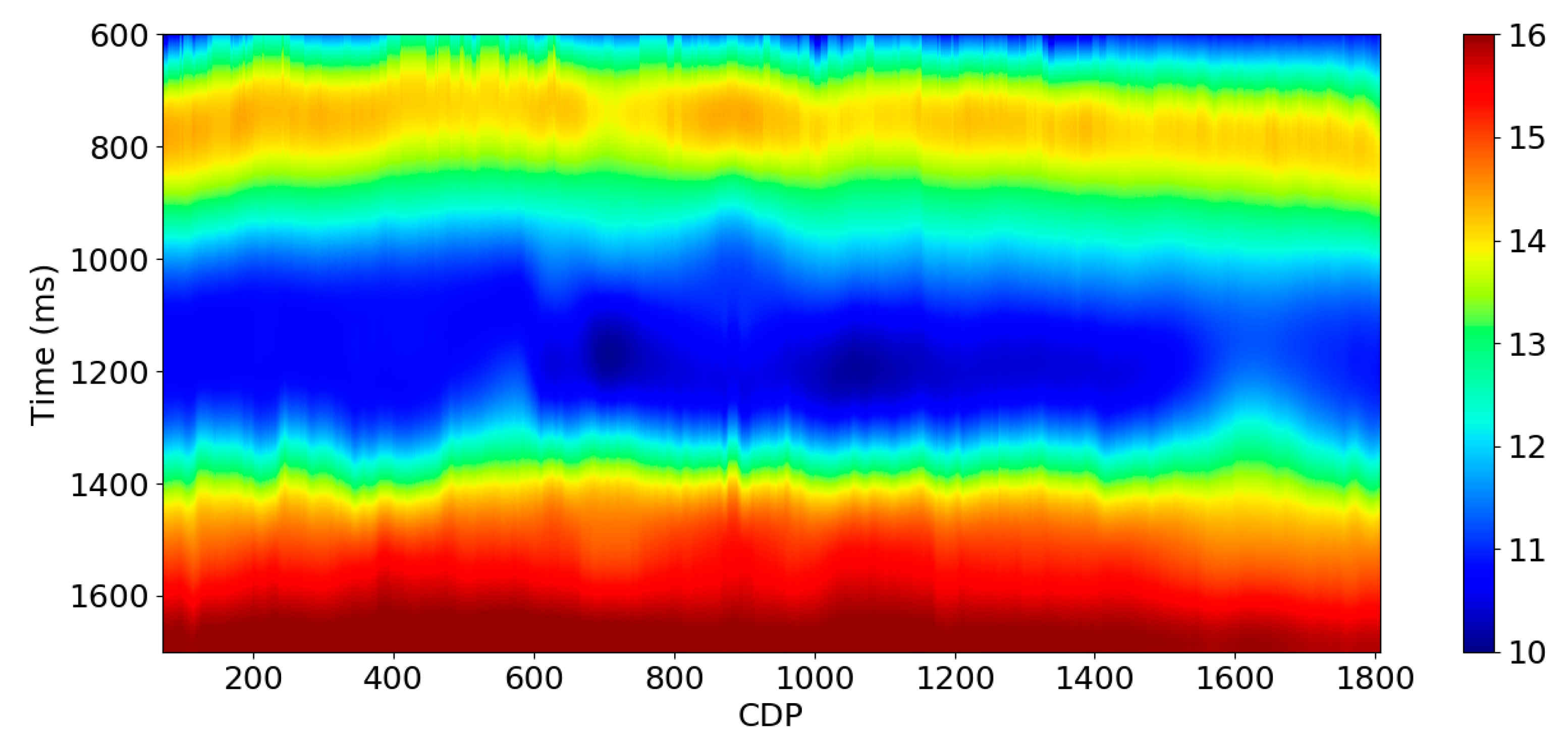
Figure 25 is the low frequency seismic data (0.0-5.0 Hz) predicted from the high frequencies of the PSTM seismic data. We use 7 wells as the training and validation set and two wells as the blind test set in this example. The average CC for these two wells is 0.67. Since this is real data, we could not evaluate the whole 2D section; however, the prediction results displayed in Figure 25 indicates that the predicted low frequency seismic section is geologically reasonable with instability at a few traces that can be removed by median filtering.

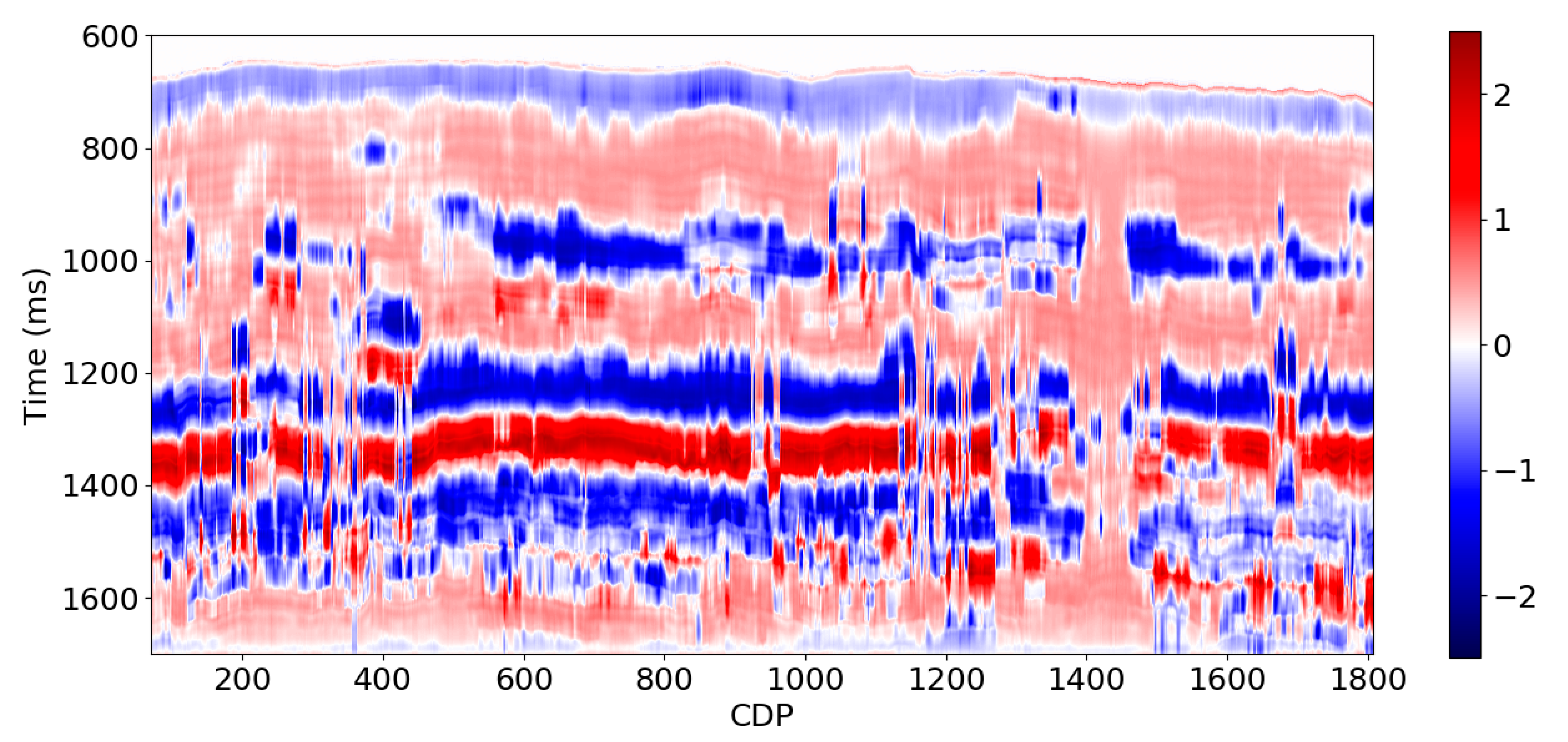
The analysis of synthetic and real data test demonstrate that the 0.0-2.0 Hz AI interpolated using well logs along the horizons could potentially provide important constraint in the prediction of 0.0-5.0 Hz AI; therefore, we use it as one of the attributes to test the proposed method (see Figure 26).

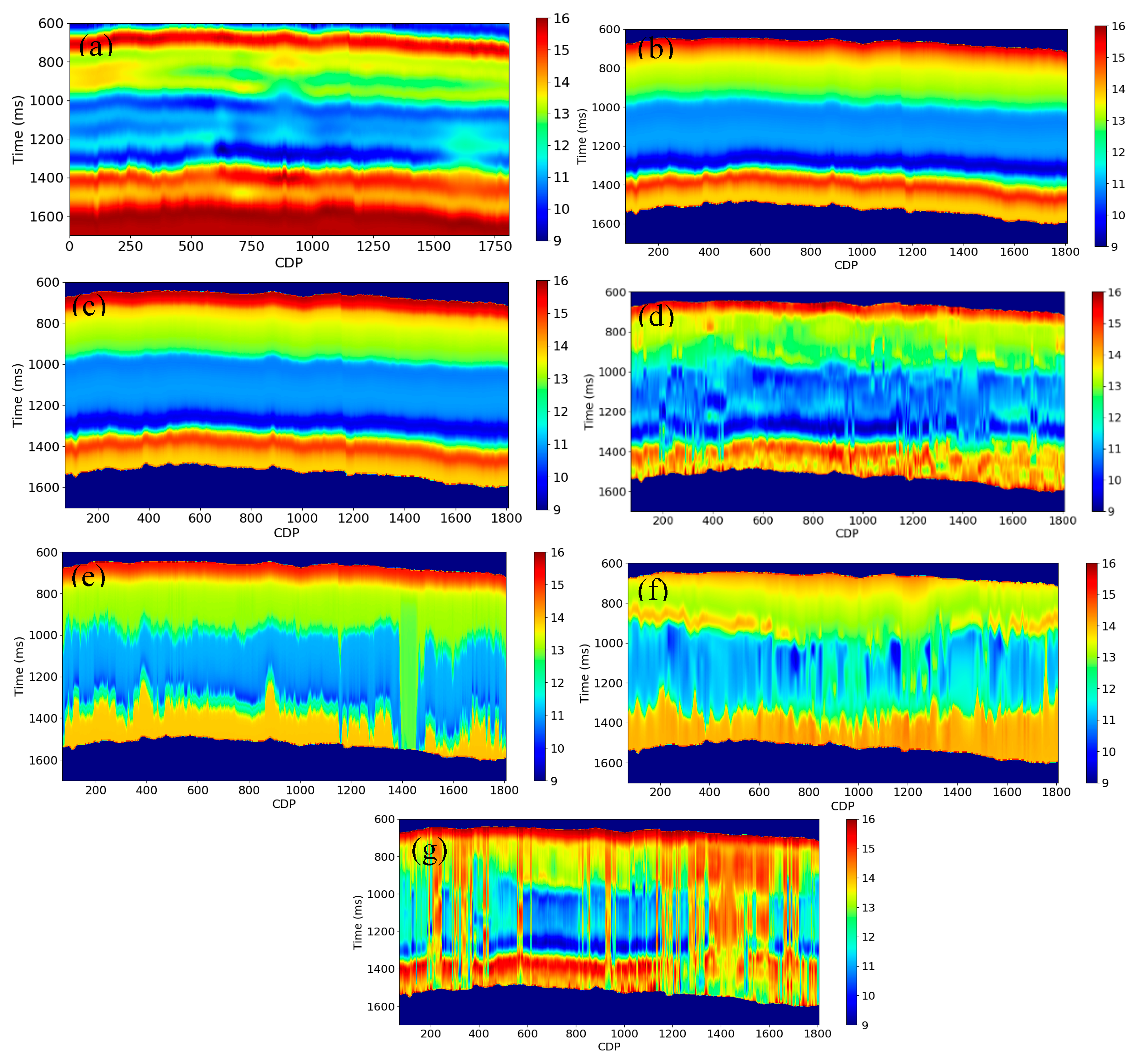
We predict the AI (0.0-5.0 Hz) using a different combination of attributes and methods using RNN for this field data set (See Table 3 and Figure 27). All the results are displayed in Figure 27, and we also summarize them in Table 3. We found that the relative geological age, interpolated AI (0.0-2.0 Hz), instantaneous amplitude, integrated instantaneous amplitude, predicted low frequency seismic data, and RMS velocity were the best attributes needed for the prediction of AI (0.0-5.0 Hz). The baseline prediction in this example is from the interpolated AI (0.0-5.0 Hz), with an average R² score of 0.52, and CC of 0.91. Note that the prediction accuracy is very different between the two blind test wells. The R² score is 0.13, and the CC is 0.83 for the blind test well 1. The R² score is 0.91, and the CC is 0.98 for the blind test well 2. This occurs very often in a real case because the interpolation of wells could be accurate when there is not lateral geological variation and vice versa. This is also why we need to introduce new attributes to help improve the prediction accuracy and stability of the low frequencies of AI.

The combination of the relative geological age, instantaneous amplitude, and predicted low frequency seismic data achieve a better performance than the baseline prediction, with an average R² score of 0.57 and CC of 0.92. The improvement is 9.6% for R² score. The benefit of this combination is that the predicted results are relatively clean. There is almost no noise in this prediction. This feature could make the prediction results stable for a variety of data sets. In addition, we could improve the prediction accuracy and stability by adding more horizons in the calculation of the relative geological age attribute.

The combination of the AI (0-2.0 Hz), predicted low frequency seismic data, RMS stack velocity also achieves a better performance than the baseline prediction, with an average R² score of 0.69 and CC of 0.95. The improvement is 32.7% for the average R² score, and 4.4% for the average CC. When we add the integrated instantaneous amplitude, the R² score improves slightly, but the CC decreases from 0.95 to 0.90. Thus, we need to decide whether to use this attribute on a case -by- case basis. The benefit of this combination is that the noise level and accuracy is intermediate compared with other cases. This combination of attributes could give a relatively stable and accurate prediction result.

The combination of the RMS stack velocity and predicted low frequency seismic data achieves the best performance in all cases, with an average R² score of 0.82 and CC of 0.94. The improvement is 57.7% for the R² score and 3.3% for CC. However, if we compare the prediction results in Figure 27g with Figure 27b and Figure 27d, we find that the results are noisy, with many stripes in the section. This can be explained by the unreliable velocity analysis. We could alleviate this issue by smoothing the RMS stack velocity and improving the RMS stack velocity accuracy by performing a more careful velocity analysis. We could also try to invert the interval velocity using tomography inversion, which could improve the velocity estimation accuracy.

4. Discussion and conclusion

Here, we showed how to predict the low frequencies of AI from various combinations of seismic attributes and geological information using deep learning. We first tested various deep learning methods to compare their performance in predicting seismic reflectivity and AI using synthetic seismic data produced by rock physics modeling. We found that CNNs are suitable for predicting the reflectivity using seismic data, but not for the impedance using reflectivity. However, we found that RNNs are suitable for both prediction tasks. In addition, the RNNs also performed well in predicting the AI using seismic data directly.

We then tested how to predict the low frequencies of AI using various combinations of attributes and methods using the Marmousi model 2. The results show that the attributes we created in this work, including the relative geological age, interval velocity, integrated instantaneous amplitude, etc., helped supply low frequencies for AI prediction. Also, we proposed a method to predict the 0.0 - 5.0 Hz low frequencies of seismic data using their high frequency components. With these attributes, we investigated how each combination of the attributes and methods performed in predicting the low frequencies of AI. We found that we can achieve good performance in predicting the low frequencies of AI by combining the new attributes, predicted low frequency seismic data, and the RNN, with an R² score of 0.93 and CC of 0.97. The biggest improvement compared with other combinations is 10.7% for R² score. We also found that we can perform better in the absolute AI inversion by adding the predicted low frequency components of AI, with the best improvement of 11.0% compared with other cases. The RNN showed some benefits over the PNN, but the improvement is not significant.

Next, we studied how each new attribute contributed to the prediction of low frequencies using convolutional synthetic seismic data created using the Marmousi model 2. The results reveal that: 1) the interval velocity, instantaneous amplitude, integrated instantaneous amplitude, predicted low frequency seismic data, and RMS velocity made a positive contribution to the prediction of the low frequencies of AI; 2) the integrated instantaneous amplitude and apparent time thickness played a less role in improving the prediction accuracy; 3) The results predicted from the combinations of the interval velocity, instantaneous amplitude, predicted low frequency seismic data, RMS velocity was better than the well logs interpolation.

Finally, we tested the proposed methods and attributes using field data from the Midland basin. We found that the relative geological age, interpolated AI (0.0 - 2.0 Hz), instantaneous amplitude, integrated instantaneous amplitude, predicted low frequency seismic data, and RMS stack velocity can help improve the prediction accuracy of the low frequencies. The combination of the relative geological age, instantaneous amplitude, and predicted low frequency seismic data made a better performance than the baseline prediction, with an average R² score of 0.52 and CC of 0.92. The average improvement for R² score is 9.6%. One of the advantages of this combination is that the predicted result is relatively clean, with only a little noise. In other words, this method could make a robust prediction compared with other methods when the signal-noise-ratio of the data is low. This method could be enhanced by adding more horizons in the attributes’ calculation.

The combination of the AI (0.0-2.0 Hz), predicted low frequency seismic data, and RMS stack velocity made a good prediction for the low frequencies, with an average R² score of 0.69 and CC of 0.95. The improvement is 32.7% for R² score and 4.4% for CC. The noise level and accuracy are intermediate compared with other cases; therefore, it could provide a relatively robust and accurate prediction result.

The combination of the RMS stack velocity and predicted low frequency seismic data achieved the best performance in all cases, with an average R² score of 0.82 and CC of 0.94, with an improvement of 57.7% for R² score and 3.3% for CC compared with the baseline prediction. One of the drawbacks of this method is that the result is noisy, with many stripes in the section caused by the low data quality and unstable velocity analysis process. Therefore, we need to be very cautious to use this method to predict the low frequencies of AI.

Author Contributions

Conceptualization, J.C. and L.J.; methodology, L.J. and Z. Z.; software, L.J.; validation, J.C., B.R. and Z.Z.; formal analysis, L.J. and Z. Z.; investigation, L.J. and Z. Z.; resources, J.C., B. R., and Z. Z.; data curation, L.J.; writing—original draft preparation, L.J.; writing—review and editing, J.C. and B. R.; visualization, L.J. and Z. Z.; supervision, J.C., B. R., Z. Z.; project administration, J.C.; funding acquisition, J.C. All authors have read and agreed to the published version of the manuscript.

Conflicts of Interest

The authors declare no conflict of interest.

References

Levy, S., and P. K. Fullagar. Reconstruction of a sparse spike train from a portion of its spectrum and application to high-resolution deconvolution. Geophysics 1981, 46, 1235–1243. [CrossRef]
Oldenburg, D. W., T. Scheuer, and S. Levy. Recovery of the acoustic impedance from reflection seismograms. Geophysics 1983, 48, 1318–1337. [CrossRef]
Sacchi, M. D., D. R. Velis, and A. H. Cominguez. Minimum entropy deconvolution with frequency-domain constraints. Geophysics 1994, 59, 938–945. [CrossRef]
Velis, D.R. Stochastic sparse-spike deconvolution. Geophysics 2008, 73, R1–R9. [Google Scholar] [CrossRef]
Zhang, R. Seismic reflection inversion by basis pursuit. Ph.D. Dissertation, University of Houston, 2010. [Google Scholar]
Liang Seismic spectral bandwidth extension and reflectivity decomposition. Ph.D. Dissertation, University of Houston, 2018.
Bianchin, L., E. Forte, and M. Pipan. Acoustic impedance estimation from combined harmonic reconstruction and interval velocity. Geophysics 2019, 84, 385–400. [CrossRef]
Wu, R. S., J. Luo, and B. Wu. Seismic envelope inversion and modulation signal model. Geophysics 2014, 79, WA13–WA24. [CrossRef]
Hu, Y.; Wu, R.S. Instantaneous-phase encoded direct envelope inversion in the time-frequency domain and the application to subsalt inversion. In SEG Technical Program Expanded Abstracts; 2020; pp. 775–779. [Google Scholar] [CrossRef]
Hu, W.; Jin, Y.; Wu, X.; Chen, J. A progressive deep transfer learning approach to cycle-skipping mitigation in FWI. In SEG Technical Program Expanded Abstracts; 2019; pp. 2348–2352. [Google Scholar]
Li, Y. E., and L. Demanet. Phase and amplitude tracking for seismic event separation. Geophysics 2015, no. 6, WD59–WD72.
Li, Y. E., and L. Demanet. Full-waveform inversion with extrapolated low-frequency data. Geophysics 2016, 81, R339–R348. [CrossRef]
Sun, H., and L. Demanet. Extrapolated full-waveform inversion with deep learning. Geophysics 2020, 85, R275–R288. [CrossRef]
Rumelhart, D. E., G. E. Hinton, and R. J. Williams. Learning representations by back-propagating errors. Nature 1986, 323, 533–536. [CrossRef]
LeCun, Y., Y. Bengio, and G. Hinton. Deep learning. Nature 2015, 521, 436–444.
Jordan, M. I., and T. M. Mitchell. Machine learning: Trends, perspectives, and prospects. Science 2015, 349, 255–260. [CrossRef] [PubMed]
Dehaene, S., H. Lau, and S. Kouider. What is consciousness, and could machines have it? Science 2017, 358, 486–492. [CrossRef] [PubMed]
Fernando, C., D. Banarse, C. Blundell, Y. Zwols, D. Ha, A. A. Rusu, A. Pritzel, and D. Wierstra. PathNet: Evolution Channels Gradient Descent in Super Neural Networks. arXiv 2017, arXiv:1701.08734v1.
George, D., W. Lehrach, K. Kansky, M. Lázaro-Gredilla, C. Laan, B. Marthi, X. Lou, Z. Meng, Y. Liu, H. Wang, A. Lavin, and D. S. Phoenix. A generative vision model that trains with high data efficiency and breaks text-based CAPTCHAs. Science 2017, 358. [CrossRef]
Sanchez-Lengeling, B., and A. Aspuru-Guzik. Inverse molecular design using machine learning: Generative models for matter engineering. Science 2018, 361, 360–365. [CrossRef]
Das, V., A. Pollack, U. Wollner, and T. Mukerji. Convolutional neural network for seismic impedance inversion. Geophysics 2019, 84, R869–R880. [CrossRef]
Sun, H., and L. Demanet. Extrapolated full-waveform inversion with deep learning. Geophysics 2020, 85, R275–R288. [CrossRef]
Hampson, D., S. S. James, and A. Q. John. Use of multiattribute transforms to predict log properties from seismic data. Geophysics 2001, 66, 220–236. [CrossRef]
Li, J., and J. P. Castagna. Support Vector Machine (SVM) pattern recognition to AVO classification. Geophysical research letters 2004, 31. [CrossRef]
Saggaf, M. M., M. N. Toksoz, and M. I. Marhoon. Seismic facies classification and identification by competitive neural networks. Geophysics 2003, 68, 1984–1999. [CrossRef]
Xie, S., R. Girshick, P. Dollar, Z. Tu, and K. He. Aggregated residual transformations for deep neural networks. arXiv 2017, arXiv:1611.05431v2.
Haris, M., G. Shakhnarovich, and N. Ukita. Deep back-projection networks for super-resolution. arXiv 2018, arXiv:1803.02735v1.
Anwar, S. and N. Barnes. Densely Residual Laplacian Super-Resolution. arXiv 2019, arXiv:1906.12021v2.
Xiong, W., X. Ji, Y. Ma, Y. Wang, N. M. AlBinHassan, M. N. Ali, and Y. Luo. Seismic fault detection with convolutional neural network. Geophysics 2018, 83, O97–O103. [CrossRef]
Wrona, T., I. Pan, R. L. Gawthorpe, and H. Fossen. Seismic facies analysis using machine learning. Geophysics 2018, 83, 83–95. [CrossRef]
Chopra, S., and K. J. Marfut. Seismic facies classification using some unsupervised machine-learning methods. In SEG Technical Program Expanded Abstracts; 2018; pp. 2056–2059.
Zhang, Z., A. D. Halpert, L. Bandura, and A. D. Coumont. Machine-learning based technique for lithology and fluid content prediction: Case study from offshore West Africa. In SEG Technical Program Expanded Abstracts; 2018; pp. 2271–2276.
Alfarraj, M., and G, AlRegib. Semi-supervised Sequence Modeling for Elastic Impedance Inversion. Interpretation 2020, 7, SE237–SE249.
Russell, B. Machine learning and geophysical inversion - A numerical study. The Leading Edge 2019, 38, 498–576. [Google Scholar] [CrossRef]
Hopfield, J.J. Neural networks and physical systems with emergent collective computational abilities. PNAS 1982, 79, 2554–2558. [Google Scholar] [CrossRef]
Martin, G.S. The Marmousi2 model, elastic synthetic data, and an analysis of imaging and AVO in a structurally complex environment. Master’s Thesis, University of Houston, 2004. [Google Scholar]
Versteeg, R. The Marmousi experience: Velocity model determination on a synthetic complex data set. The Leading Edge 1994, 13, 927–936. [Google Scholar] [CrossRef]
Bianchin, L., E. Forte, and M. Pipan. Acoustic impedance estimation from combined harmonic reconstruction and interval velocity. Geophysics 2019, 84, 385–400. [CrossRef]
Yilmaz, O. Seismic Data Analysis: Processing, Inversion, and Interpretation of Seismic Data; Society of Exploration Geophysicists: Tulsa, OK, 2001; 1028p. [Google Scholar]
Robinson, K. Petroleum geology and hydrocarbon plays of the Permain basin petroleum province west Texas and southeast New Mexico: U.S. Geological Survey, 1988.

Figure 1. Architecture of CNNs used in this study.

Figure 3. The reflectivity is predicted from seismic data using different methods. (a) Training result from CNN. (b) Test result from CNN. (c) Training result from RNN. (d) Test result from RNN. The hyperparameters used in this test are: batch size = 2, maximum epoch = 300, and learning rate = 0.005. The activation function used in this test is tanh function.

Figure 4. The AI predicted from reflectivity using different methods. (a) Training result from CNN. (b) Test result from CNN. The CC is 0.70. (c) Training result from RNN. (d) Test result from RNN.

Figure 5. The AI predicted directly using seismic data. (a) Training result from CNN. (b) Test result from CNN. (c) Training result from RNN. (d) Test result from RNN.

Figure 6. (a) AI. (b) PSTM seismic data.

Figure 7. (a) The horizons and faults extracted from the Marmousi model 2. (b) Relative geological age attribute created using the horizons and faults.

Figure 8. (a) True depth. (b) The depth attribute estimated using the time-depth relationship at pseudo well locations along the horizons.

Figure 9. (a) True interval velocity. (b) Interval velocity calculated using the depth attribute.

Figure 10. (a) Seismic data (black) and instantaneous amplitude (red). (b) Instantaneous amplitude (black) (same as the red curve in (a)) and integrated instantaneous amplitude (red). (c) Instantaneous amplitude (black) and peaks (red dot). (d) Instantaneous amplitude (black) and peaks (red dot) and apparent time thickness (green).

Figure 11. (a) PSTM seismic data (black). (b) Instantaneous amplitude. (c) Integrated instantaneous amplitude. (d) Apparent time thickness.

Figure 12. (a) 5.0-40.0 Hz PSTM seismic data. (b) Synthetic seismic data created using convolutional model (0.0-5.0 Hz). (c) 0.0-5.0 Hz seismic data predicted using the data in (a).

Figure 14. (a) Training result from PNN. The CC is 1.0 and R² score is 0.99. (b) Validation result from PNN. The CC is 0.98 and R² score is 0.95. (c) Training result from RNN. The CC is 1.0 and R² score is 0.99. (d) Validation result from RNN. The CC is 0.97 and R² score is 0.95.

Figure 15. Prediction results from various kinds of combinations of attributes and methods. (a) True AI (0.0-5.0 Hz). (b) AI (0.0-5.0 Hz) predicted from the conventional seismic attributes using PNN. (c) AI (0.0-5.0 Hz) predicted from the new and conventional attributes using PNN. (d) AI (0.0-5.0 Hz) predicted from the new and conventional attributes using RNN. (e) AI (0.0-5.0 Hz) predicted from the predicted low frequency seismic data and new attributes using RNN.

Figure 16. (a) Interval velocity from Marmousi model 2. (b) RMS velocity calculated using Dix equation.

Figure 17. (a) 0.0-5.0 Hz AI (True). (b) AI (0.0-5.0 Hz) predicted using RMS velocity.

Figure 18. (a) 0.0-10.0 Hz AI (True). (b) AI (0-10.0 Hz) predicted using RMS velocity.

Figure 19. (a) 0-10.0 Hz AI (True). (b) AI (0-10.0 Hz) predicted using the RMS velocity and 5.0-10.0 Hz PSTM seismic data using RNN (10 wells). (c) AI (0-10.0 Hz) predicted using the RMS velocity and 5-10 Hz PSTM seismic data using RNN (5 wells).

Figure 20. Geological map of Permian Basin. The red dashed box is the general location of the 3D seismic data.

Figure 21. Seismic arbitrary line going through all the wells (PSTM).

Figure 22. (a) The horizons interpreted on the PSTM seismic data from Figure 21. (b) Relative geological age attribute calculated from the horizons in (a).

Figure 23. (a) Seismic data (black) and instantaneous amplitude (red). (b) Instantaneous amplitude (black) and integrated instantaneous amplitude (red). (c) Instantaneous amplitude (black) and peaks (red dot). (d) Instantaneous amplitude (black) and peaks (red dot) and apparent time thickness (green).

Figure 24. (a) PSTM seismic data. (b) Instantaneous amplitude. (c) Integrated instantaneous amplitude. (d) Apparent time thickness.

Figure 25. 0.0-5.0 Hz seismic data predicted using bandlimited PSTM seismic data.

Figure 26. 0.0-2.0 Hz AI interpolated using well logs along horizons.

Figure 27. (a) AI (0.0-5.0 Hz) calculated using the well logs interpolation along horizons. (b) AI (0.0-5.0 Hz) predicted using the relative geological age and predicted low frequency seismic data. (c) AI (0.0-5.0 Hz) predicted using the relative geological age, predicted low frequency seismic data, and instantaneous amplitude. (d) AI (0.0-5.0 Hz) predicted using the AI (0-2.0 Hz), predicted low frequency seismic data, and RMS velocity. (e) AI (0.0-5.0 Hz) predicted using the AI (0-2.0 Hz), predicted low frequency seismic data, RMS velocity, and integrated instantaneous amplitude. (f) AI (0.0-5.0 Hz) using the RMS stack velocity. (g) AI (0.0-5.0 Hz) using the RMS velocity and predicted low frequency seismic data.

Table 1. Validation summary for the AI (0.0-5.0 Hz) predicted using various kinds of combinations of attributes and methods. The R² score and CC in this table are the average value calculated using the whole 2-D line.

Attributes and Methods	AI (0.0-5.0 Hz)
Attributes and Methods	R² score	CC
Conventional attributes + PNN	0.84	0.94
New and conventional attributes + Linear regression	0.87	0.94
New and conventional attributes + PNN	0.91	0.96
New and conventional attributes + RNN	0.90	0.95
New attributes and predicted low frequency seismic data + RNN	0.93	0.97

Table 2. Validation summary for the AI (full band) predicted using various kinds of combinations of attributes and methods. The R² score and CC in this table are the average value calculated using the whole 2-D line.

Attributes and Methods	AI (absolute)
Attributes and Methods	R² score	CC
Conventional attributes + PNN	0.82	0.93
Raw seismic + RNN	0.82	0.93
Predicted low frequency components and conventional attributes + PNN	0.88	0.94
Predicted low frequency components+ Raw seismic + RNN	0.90	0.95
Predicted low frequency components from RNN + Raw seismic + RNN	0.91	0.96

Table 3. Validation summary for the AI (0.0 - 5.0 Hz) predicted using various kinds of combinations of attributes and methods. Test 1 is the result of the blind test well 1, and test 2 is the result of the blind test well 2.

Attributes/Methods	AI (0.0-5.0 Hz)
Attributes/Methods	Test 1 R² score	Test 1 CC	Test 2 R² score	Test 2 CC	Average R² score	Average CC
Well logs interpolation along horizons	0.13	0.83	0.91	0.98	0.52	0.91
Relative geological age + Instantaneous amplitude + Integrated instantaneous amplitude + Apparent thickness	0.47	0.89	0.14	0.49	0.30	0.69
Relative geological age + Predicted low frequency seismic data	0.19	0.82	0.93	0.98	0.56	0.90
Relative age + Predicted low frequency seismic data + Instantaneous amplitude	0.23	0.86	0.92	0.98	0.57	0.92
Relative geological age + RMS stack velocity + Predicted low frequency seismic data + Instantaneous amplitude	0.41	0.90	0.82	0.93	0.61	0.91
AI (0-2.0 Hz) (interpolated using well logs) + Instantaneous amplitude	0.38	0.89	0.94	0.98	0.66	0.94
AI (0-2.0 Hz) (interpolated using well logs) + RMS stack velocity	0.16	0.83	0.93	0.97	0.55	0.90
AI (0-2.0 Hz) + Predicted low frequency seismic data	0.42	0.92	0.94	0.98	0.68	0.95
AI (0-2.0 Hz) + Predicted low frequency seismic data + RMS stack velocity	0.43	0.93	0.95	0.98	0.69	0.95
AI (0-2.0 Hz) + Predicted low frequency seismic data + RMS stack velocity + Instantaneous amplitude	0.39	0.93	0.91	0.98	0.65	0.95
AI (0-2.0 Hz) + RMS stack velocity + Predicted low frequency seismic data + Integrated instantaneous amplitude	0.63	0.88	0.80	0.92	0.71	0.90
AI (0-2.0 Hz) + Integrated instantaneous amplitude	0.59	0.91	0.45	0.68	0.52	0.80
RMS stack velocity	0.85	0.93	0.71	0.94	0.79	0.94
RMS stack velocity + Predicted low frequency seismic data	0.81	0.91	0.82	0.97	0.82	0.94

Disclaimer/Publisher’s Note: The statements, opinions and data contained in all publications are solely those of the individual author(s) and contributor(s) and not of MDPI and/or the editor(s). MDPI and/or the editor(s) disclaim responsibility for any injury to people or property resulting from any ideas, methods, instructions or products referred to in the content.

© 2023 by the authors. Licensee MDPI, Basel, Switzerland. This article is an open access article distributed under the terms and conditions of the Creative Commons Attribution (CC BY) license (http://creativecommons.org/licenses/by/4.0/).

Copyright: This open access article is published under a Creative Commons CC BY 4.0 license, which permit the free download, distribution, and reuse, provided that the author and preprint are cited in any reuse.

MDPI Initiatives

Important Links

Choose an area of interest and we will send you notifications of new preprints at your preferred frequency.

Disclaimer