Submitted:
17 August 2023
Posted:
21 August 2023
You are already at the latest version
Abstract
Keywords:
1. Introduction
2. Literature Review
3. Study Area and Data Sources
4. Methodology
5. Results and Discussions
6. Conclusions and Future Work
Author Contributions
Funding
Institutional Review Board Statement
Informed Consent Statement
Data Availability Statement
Conflicts of Interest
References
- Lord, D.; Washington, S.P.; Ivan, J.N. Poisson, Poisson-gamma and zero-inflated regression models of motor vehicle crashes: Balancing statistical fit and theory. Accident Analysis & Prevention 2005, 37, 35–46. [Google Scholar] [CrossRef]
- AASHTO. Highway Safety Manual; 2010. [Google Scholar]
- Abdel-Aty, M.A.; Lee, C.; Park, J.; Wang, J.H.; Abuzwidah, M.; Al-Arifi, S. Validation and application of highway safety manual (part D) in Florida; Technical report; 2014. [Google Scholar]
- Alluri, P.; Saha, D.; Liu, K.; Gan, A. Improved processes for meeting the data requirements for implementing the Highway Safety Manual (HSM) and Safety Analyst in Florida; Technical report; 2014. [Google Scholar]
- Srinivasan, R.; Carter, D. Development of Safety Performance Functions for North Carolina; 2011; p. 88. [Google Scholar]
- Wang, J.H.; Abdel-Aty, M.; Lee, J. Examination of the Transferability of Safety Performance Functions for Developing Crash Modification Factors: Using the Empirical Bayes Method. Transportation Research Record: Journal of the Transportation Research Board 2016, 2583, 73–80. [Google Scholar] [CrossRef]
- Poch, M.; Mannering, F. Negative Binomial Analysis of Intersection-Accident Frequencies. Journal of Transportation Engineering 1996, 122, 105–113. [Google Scholar] [CrossRef]
- Lu, J.; Haleem, K.; Alluri, P.; Gan, A.; Liu, K. Developing local safety performance functions versus calculating calibration factors for SafetyAnalyst applications: A Florida case study. Safety Science 2014, 65, 93–105. [Google Scholar] [CrossRef]
- Ulak, M.B.; Ozguven, E.E.; Karabag, H.H.; Ghorbanzadeh, M.; Moses, R.; Dulebenets, M. Development of Safety Performance Functions for Restricted Crossing U-Turn Intersections. Journal of Transportation Engineering, Part A: Systems 2020, 146. [Google Scholar] [CrossRef]
- Young, J.; Park, P.Y. Benefits of small municipalities using jurisdiction-specific safety performance functions rather than the Highway Safety Manual’s calibrated or uncalibrated safety performance functions. Canadian Journal of Civil Engineering 2013, 40, 517–527. [Google Scholar] [CrossRef]
- Srinivasan, R.; Colety, M.; Bahar, G.; Crowther, B.; Farmen, M. Estimation of Calibration Functions for Predicting Crashes on Rural Two-Lane Roads in Arizona. Transportation Research Record: Journal of the Transportation Research Board 2016, 2583, 17–24. [Google Scholar] [CrossRef]
- Farid, A.; Abdel-Aty, M.; Lee, J. A new approach for calibrating safety performance functions. Accident Analysis and Prevention 2018, 119, 188–194. [Google Scholar] [CrossRef] [PubMed]
- Dong, Q.; Jiang, X.; Huang, B.; Richards, S.H. Analyzing Influence Factors of Transverse Cracking on LTPP Resurfaced Asphalt Pavements through NB and ZINB Models. Journal of Transportation Engineering 2013, 139, 889–895. [Google Scholar] [CrossRef]
- Sun, C.; Brown, H.; Edara, P.; Claros, B.; Nam, K. Calibration of the HSM’s SPFs for Missouri; Publication CMR14-007; Missouri Department of Transportation, 2014. [Google Scholar]
- Kweon, Y.j.; Lim, I.k. Development of Safety Performance Functions for Multilane Highway and Freeway Segments Maintained by the Virginia Department of Transportation. Technical report, 2014.
- Donnell, E.T.; Gayah, V.V.; Li, L. Regionalized Safety Performance Functions. Final report for the Pennsylvania Department of Transportation, FHWA-PA-2016-001-PSU WO 17 2016.
- Khattak, A.; Ahmad, N.; Mohammadnazar, A.; MahdiNia, I.; Wali, B.; Arvin, R. Highway Safety Manual Safety Performance Functions& Roadway Calibration Factors: Roadway Segments Phase 2, Part 2020.
- Al-Deek, H.; Sandt, A.; Gamaleldin, G.; McCombs, J.; Blue, P. A Roadway Context Classification Approach for Developing Safety Performance Functions and Determining Traffic Operational Effects for Florida Intersections. Technical report, 2020.
- Kitali, A.E.; Sando, T.; Castro, A.; Kobelo, D.; Mwakalonge, J. Using Crash Modification Factors to Appraise the Safety Effects of Pedestrian Countdown Signals for Drivers. Journal of Transportation Engineering, Part A: Systems 2018, 144. [Google Scholar] [CrossRef]
- Brimley, B.; Saito, M.; Schultz, G. Calibration of highway safety manual safety performance function: Development of New Models for Rural Two-Lane Two-Way Highways, 2012. [CrossRef]
- Gross, F.; Persaud, B.; Lyon, C. A Guide to Developing Quality Crash Modification Factors. Technical report, 2010.
- Srinivasan, R.; Bauer, K. Safety Performance Function Development Guide: Developing JurisdictionSpecific SPFs. Technical report, 2013.
- Hauer, E. Overdispersion in modelling accidents on road sections and in Empirical Bayes estimation. Accident Analysis & Prevention 2001, 33, 799–808. [Google Scholar] [CrossRef]
- Hauer, E.; Harwood, D.W.; Council, F.M.; Griffith, M.S. Estimating Safety by the Empirical Bayes Method: A Tutorial. Transportation Research Record: Journal of the Transportation Research Board 2002, 1784, 126–131. [Google Scholar] [CrossRef]
- Lord, D.; Mannering, F. The statistical analysis of crash-frequency data: A review and assessment of methodological alternatives. Transportation Research Part A: Policy and Practice 2010, 44, 291–305. [Google Scholar] [CrossRef]
- Farid, A.; Abdel-Aty, M.; Lee, J. Comparative analysis of multiple techniques for developing and transferring safety performance functions. Accident Analysis & Prevention 2019, 122, 85–98. [Google Scholar] [CrossRef]
- Persaud, B.; Lan, B.; Lyon, C.; Bhim, R. Comparison of empirical Bayes and full Bayes approaches for before–after road safety evaluations. Accident Analysis & Prevention 2010, 42, 38–43. [Google Scholar] [CrossRef]
- Das, S.; Tsapakis, I.; Khodadadi, A. Safety performance functions for low-volume rural minor collector two-lane roadways. IATSS Research 2021, 45, 347–356. [Google Scholar] [CrossRef]
- Wood, G. Generalised linear accident models and goodness of fit testing. Accident Analysis & Prevention 2002, 34, 417–427. [Google Scholar] [CrossRef]
- Lord, D. Modeling motor vehicle crashes using Poisson-gamma models: Examining the effects of low sample mean values and small sample size on the estimation of the fixed dispersion parameter. Accident Analysis & Prevention 2006, 38, 751–766. [Google Scholar] [CrossRef]
- Florida Department of Transportation (FDOT). Statewide Traffic Data Files, 2022.
- FDOT Safety Office. FDOT Highway Safety Manual User Guide 2015, 2015.
- Faraway, J.J. Extending the Linear Model with R; Chapman and Hall/CRC, 2016. [Google Scholar] [CrossRef]
- Florida Department of Transportation. FDOT Context Classification Guide. Technical report, 2020.
- Gamaleldin, G.; Al-Deek, H.; Sandt, A.; El-Urfali, A.; Kayes, M.I.; Gamero, V. Roadway Context Classification Approach for Developing Regional Safety Performance Functions for Florida Intersections. Transportation Research Record 2020, 2674, 191–202. [Google Scholar] [CrossRef]
- Tayebikhorami, S.; Sacchi, E. Validation of Machine Learning Algorithms as Predictive Tool in the Road Safety Management Process: Case of Network Screening. Journal of Transportation Engineering, Part A: Systems 2022, 148. [Google Scholar] [CrossRef]


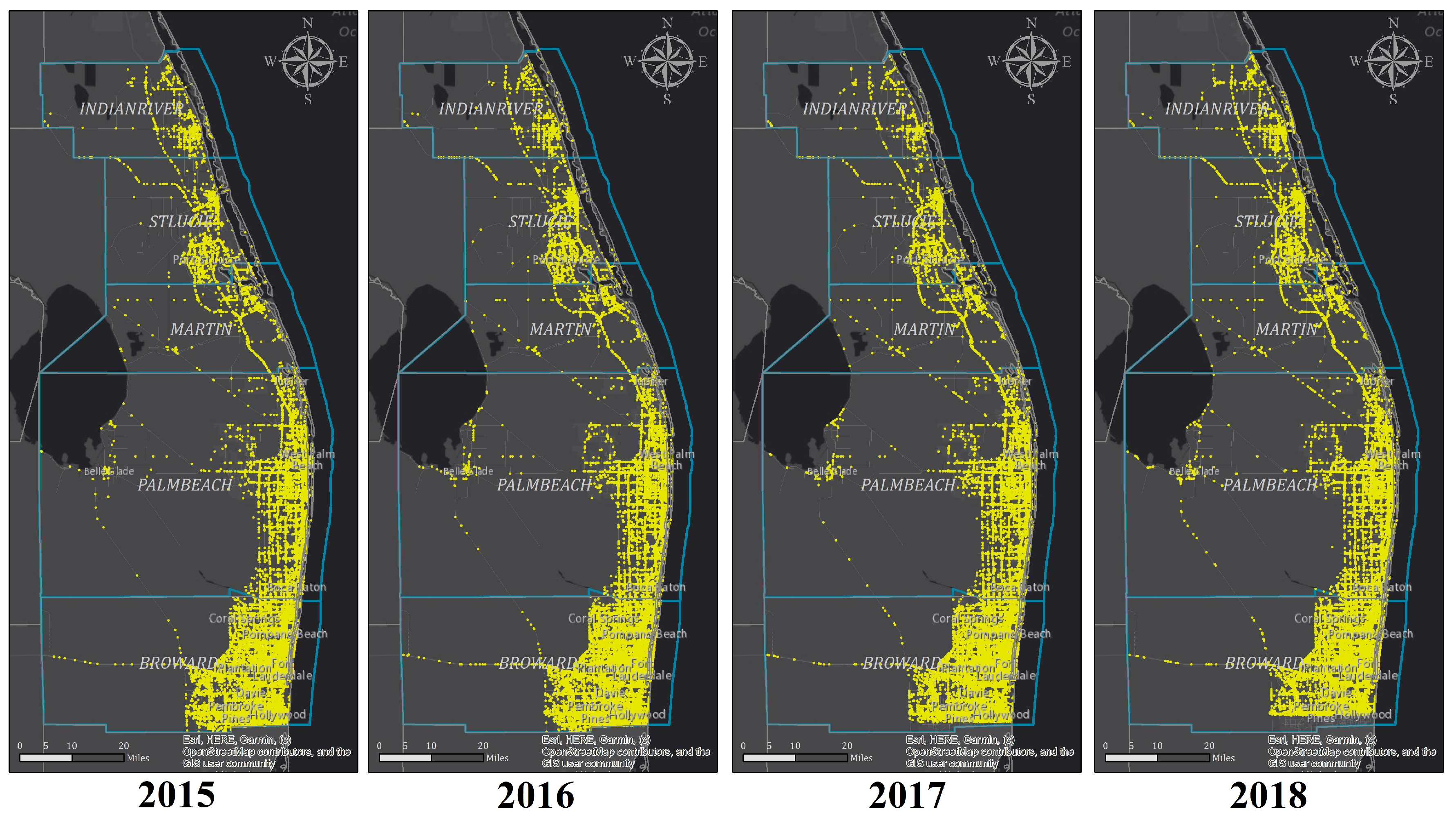
| Crash Type | 2015 | 2016 | 2017 | 2018 |
|---|---|---|---|---|
| All Crash in Florida | 374,342 | 395,785 | 402,385 | 403,626 |
| All Crash in District 4 | 76,025 | 85,611 | 83,688 | 86,596 |
| All Considered Crash* | 31,013 | 37,003 | 34,538 | 38,630 |
| All Considered Crash on U4D | 6,154 | 7,538 | 6,474 | 6,289 |
| U4D KABC Crash** | 1,334 | 1,647 | 1,440 | 1,371 |
| U4D PDO Crash*** | 3,870 | 4,881 | 4,163 | 4,113 |
| KABCO Scale | Crash Type (Level of Injury) | Overdispersion Parameter | ||
|---|---|---|---|---|
| KABCO | Total Crashes | −12.34 | 1.36 | 1.32 |
| KABC | Fatal-and-Injury Crashes | −12.76 | 1.28 | 1.31 |
| PDO | Property Damage Only Crashes | −12.81 | 1.38 | 1.34 |
| Diagnostic Test | 10 miles | 15 miles |
|---|---|---|
| GOF test p-value | 0.0204 | 0.0054 |
| Estimated k | 0.6469 | 0.6600 |
| Zero Inflation p-value | 0.9851 | 0.2623 |
| HSM k-value | 1.32 | 1.32 |
Disclaimer/Publisher’s Note: The statements, opinions and data contained in all publications are solely those of the individual author(s) and contributor(s) and not of MDPI and/or the editor(s). MDPI and/or the editor(s) disclaim responsibility for any injury to people or property resulting from any ideas, methods, instructions or products referred to in the content. |
© 2023 by the authors. Licensee MDPI, Basel, Switzerland. This article is an open access article distributed under the terms and conditions of the Creative Commons Attribution (CC BY) license (http://creativecommons.org/licenses/by/4.0/).


