1. Introduction
The implementation of Customer Relationship Management (CRM) is a strategic approach to managing and enhancing relationships between businesses and their customers. Through the utilization of CRM, businesses can establish an infrastructure that fosters long-term and loyal customers. This concept is relevant across various industries, such as banking [
1,
2,
3,
4], insurance companies [
5], and telecommunications [
6,
7,
8,
9,
10,
11,
12,
13,
14,
15], to name a few. A key objective of CRM is customer retention, as studies have demonstrated that the cost of acquiring new customers can be 20 times higher than retaining existing ones [
1]. As a result, it is imperative for businesses to develop practical tools to achieve this goal. In recent years, various Machine Learning (ML) methods have been proposed for constructing a churn model, including Artificial Neural Networks (ANN) [
8,
9,
16,
17,
18], Decision Trees [
8,
9,
11,
13,
16,
17], Random Forests [
19,
20], Logistic Regression (LR) [
9,
13], Support Vector Machines (SVM) [
17], and Rough Set Approach [
21], among others.
In the following paragraphs, an overview is provided of five of the most commonly utilized techniques. Additionally, three prominent boosting algorithms, namely eXtreme Gradient Boosting (XGBoost), Categorical Boosting (CatBoost), and Light Gradient Boosting Machine (LightGBM), were selected for use. Ensemble techniques [
22], specifically boosting and bagging algorithms, have become the prevalent choice for addressing classification problems [
23,
24], particularly in the realm of churn prediction [
25,
26], due to their demonstrated high effectiveness.
The remainder of the paper is organized as follows:
Section 2 presents an introduction to machine learning techniques,
Section 3 delves into the examination of sampling methods,
Section 4 defines evaluation metrics, simulation results are presented in
Section 5, and the paper concludes in
Section 6.
2. Machine Learning Techniques
In the following, an overview is provided of the most frequently utilized techniques for addressing the issue of churn prediction, including Artificial Neural Network, Decision Tree, Support Vector Machine, Random Forest, Logistic Regression, and three advanced gradient boosting techniques, specifically XGBoost, LightGBM, and CatBoost.
A. Artificial Neural Network
Artificial Neural Network (ANN) is a widely employed technique for addressing complex issues such as the churn prediction problem [
27]. ANNs are structures composed of interconnected units that are modeled after the human brain. They can be utilized with various learning algorithms to enhance the machine learning process and can take both hardware and software forms. One of the most widely utilized models is the Multi-Layer Perceptron, which is trained using the Back-Propagation Network (BPN) algorithm. Research has demonstrated that ANNs possess superior performance compared to Decision Trees (DTs) [
27], and have been shown to exhibit improved performance when compared to Logistic Regression (LR) and DTs in the context of churn prediction [
28].
B. Support Vector Machine
The technique of Support Vector Machine (SVM) was first introduced by authors in [
29]. It is classified as a supervised learning technique that utilizes learning algorithms to uncover latent patterns within data. A popular method for improving the performance of SVMs is the utilization of kernel functions [
8]. In addressing customer churn problems, SVM may exhibit superior performance in comparison to Artificial Neural Networks (ANNs) and Decision Trees (DTs) based on the specific characteristics of the data [
17,
30].
For this study, we utilize both the Gaussian Radial Basis kernel function (RBF-SVM) and the Polynomial kernel function (Poly-SVM) for the Support Vector Machine (SVM) technique. These kernel functions are among the various options available for use with SVM.
For two samples
and
, the RBF kernel is defined as follows:
Where can be the squared Euclidean distance and is a free parameter.
For two samples
and
, the d-degree polynomial kernel is defined as follows:
Where and is the polynomial degree.
C. Decision Tree
A Decision Tree (DT) is a representation of all potential decision pathways in the form of a tree structure [
31,
32]. As Berry and Linoff stated, "a Decision Tree is a structure that can be used to divide up a large collection of records into successively smaller sets of records by applying a sequence of simple decision rules" [
33]. Though they may not be as efficient in uncovering complex patterns or detecting intricate relationships within data, DTs may be used to address the customer churn problem, depending on the characteristics of the data. In DTs, class labels are indicated by leaves and the conjunctions between various features are represented by branches.
D. Logistic Regression
Logistic Regression (LR) is a classification method that falls under the category of probabilistic statistics. It can be employed to address the churn prediction problem by making predictions based on multiple predictor variables. In order to obtain high accuracy, which can sometimes be comparable to that of Decision Trees (DTs) [
10], it is often beneficial to apply pre-processing and transformation techniques to the original data prior to utilizing LR.
3. Ensemble Learning
Ensemble learning is one of the widely utilized techniques in machine learning for combining the outputs of multiple learning models (often referred to as base learners) into a single classifier [
34]. In ensemble learning, it is possible to combine various weak machine learning models (base learners) to construct a stronger model with more accurate predictions [
35,
36]. Currently, ensemble learning methods are widely accepted as a standard choice for enhancing the accuracy of machine learning predictors [
35]. Bagging and boosting are two distinct types of ensemble learning techniques that can be utilized to improve the accuracy of machine learning predictors [
36].
A. Bagging
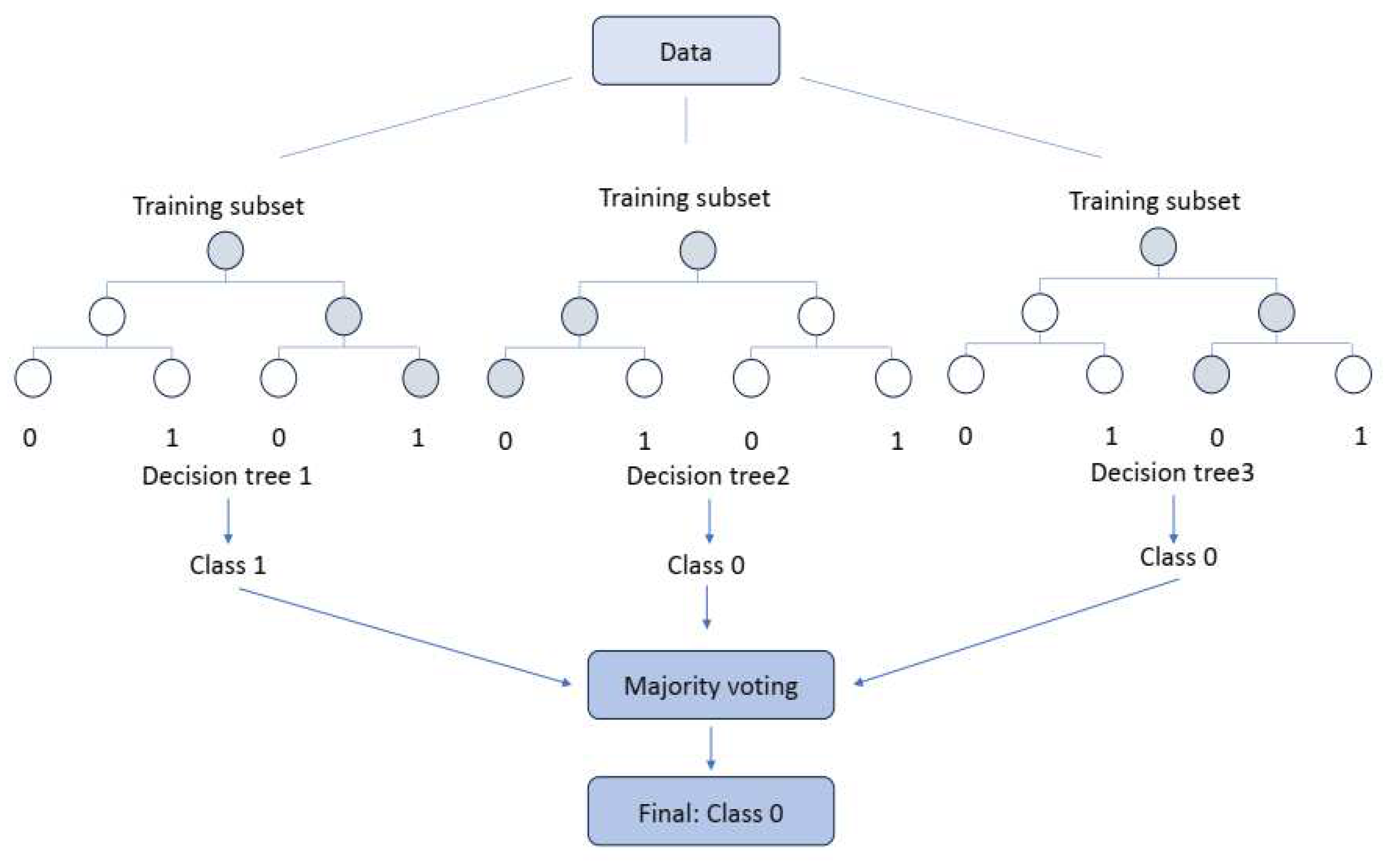
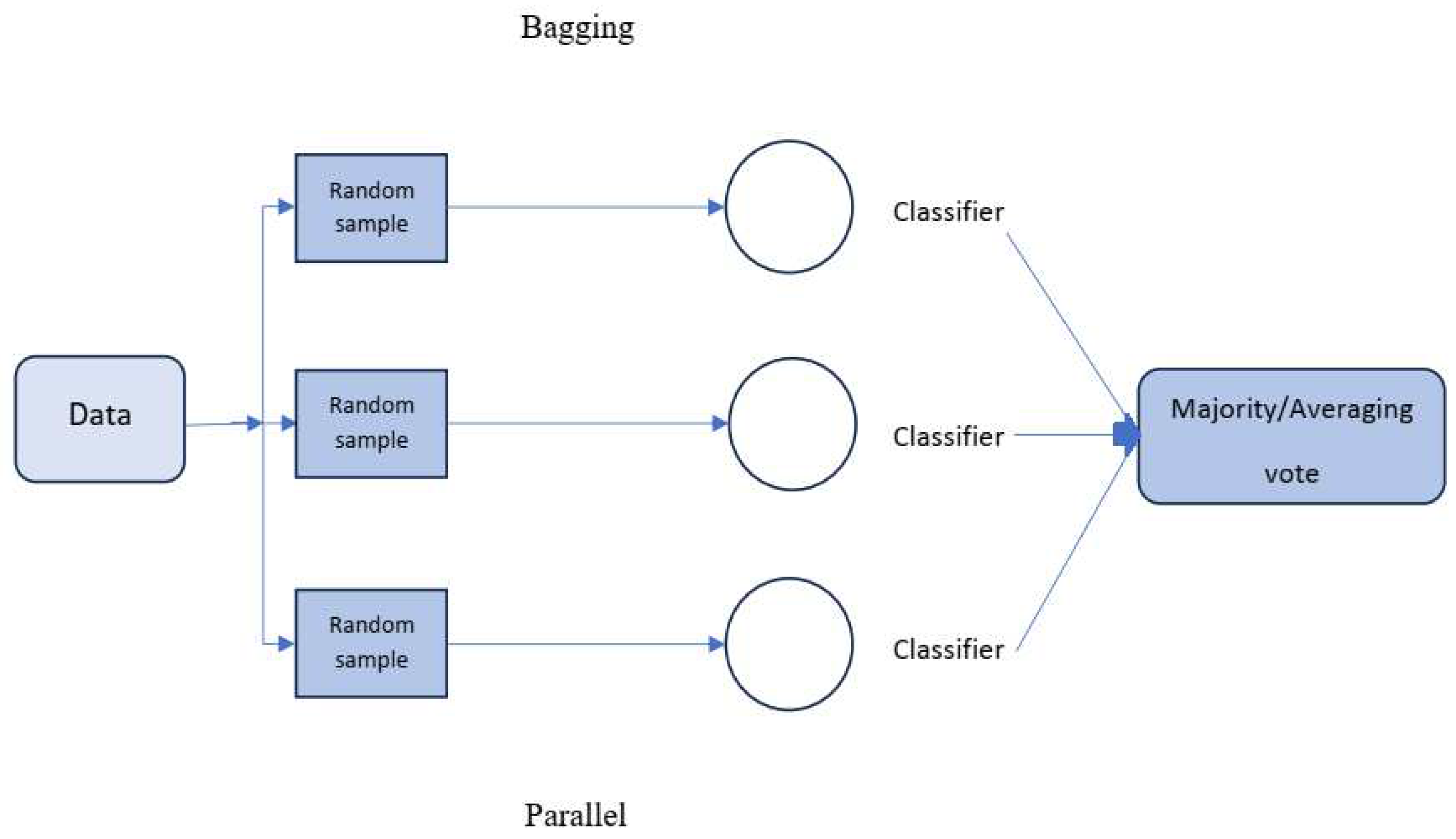
As depicted in
Figure 1, in the bagging technique, the training data is partitioned into multiple subset sets, and the model is trained on each subset. The final prediction is then obtained by combining all individual outputs through majority voting (in classification problems) or average voting (in regression problems) [
36,
37,
38].
B. Random Forest
The concept of Random Forest was first introduced by Ho in 1995 [
19] and has been the subject of ongoing improvement by various researchers. One notable advancement in this field was made by Leo Breiman in 2001 [
20]. Random Forests are an ensemble learning technique for classification tasks that employs a large number of Decision Trees in the training model. The output of Random Forests is a class that is selected by the majority of the trees. In general, Random Forests exhibit superior performance compared to Decision Trees (DTs), however, the performance can be influenced by the characteristics of the data.
Random Forests utilize the bagging technique for their training algorithm. In greater detail, the Random Forests operate as follows: For a training set , bagging is repeated B times, and each iteration selects a random sample with replacement from , and fits trees to the samples.:
1- Sample training examples;
2- Train a classification tree (in the case of churn problems) on the samples .
After the training phase, Random Forests can predict unseen samples
by taking the majority vote from all the individual classification trees
.
C. Boosting
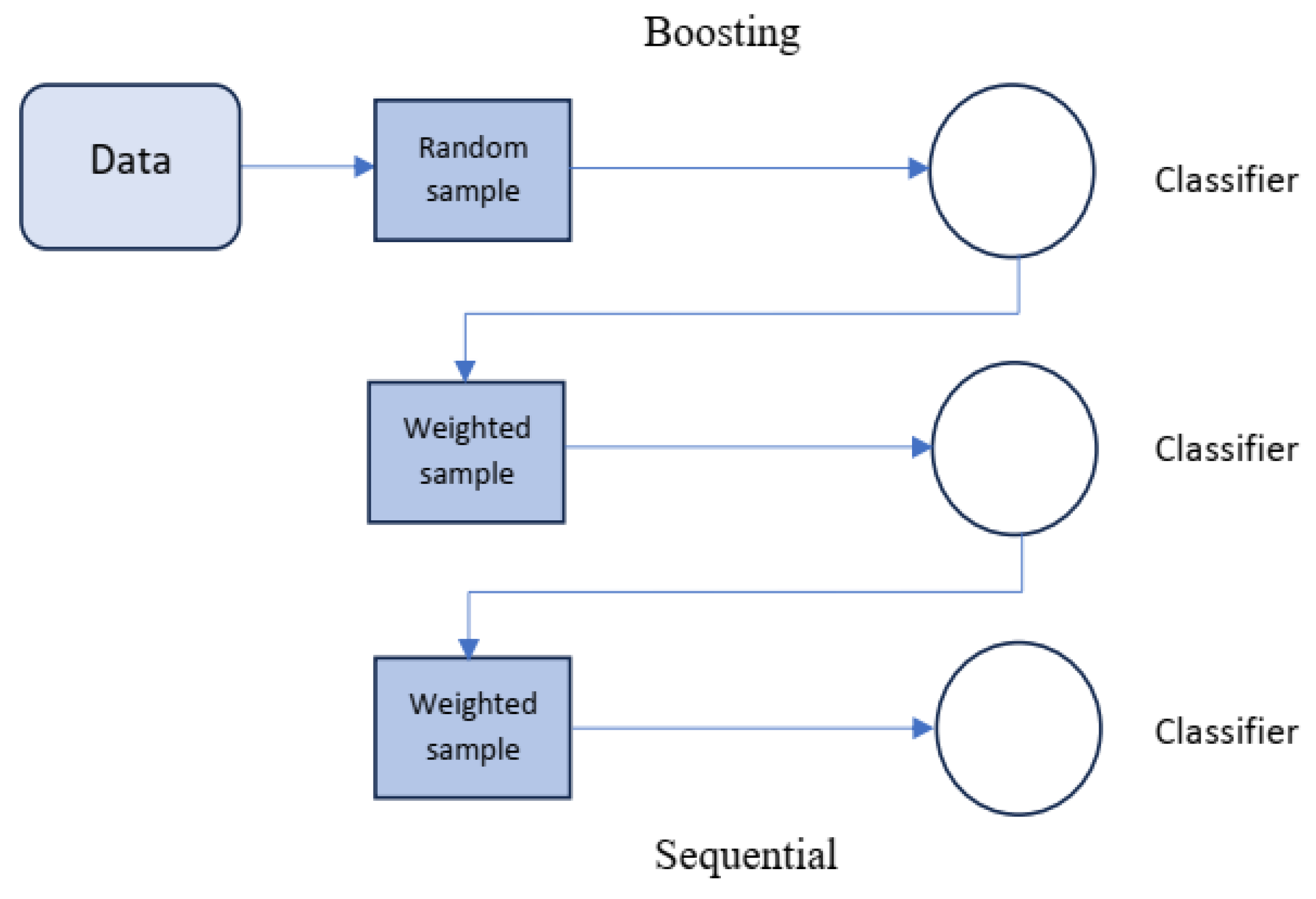
Boosting is another method for combining multiple base learners to construct a stronger model with more accurate predictions. The key distinction between bagging and boosting is that bagging uses a parallel approach to combine weak learners, while boosting methods utilize a sequential approach to combine weak learners and derive the final prediction, as shown in
Figure 2. Like the bagging technique, boosting improves the performance of machine learning predictors and in addition, it reduces the bias of the model [
36].
Figure 2.
Visualization of the Random Forest classifier.
Figure 2.
Visualization of the Random Forest classifier.
Figure 3.
Visualization of the boosting approach.
Figure 3.
Visualization of the boosting approach.
D. The Famous Trio: XGBoost, LightGBM, CatBoost
Recently, researchers have presented three effective gradient-based approaches using decision trees: CatBoost, LightGBM, and XGBoost. These new approaches have demonstrated successful applications in academia, industry, and competitive machine learning [
39]. Utilizing gradient boosting techniques, solutions can be constructed in a stagewise manner, and the over-fitting problem can be addressed through the optimization of loss functions. For example, given a loss function
and a custom base-learner
h(x, θ) (e.g., decision tree), the direct estimation of parameters can be challenging. Thus, an iterative model is proposed, which is updated at each iteration with the selection of a new base-learner function
h(x, θt), where the increment is directed by:
Hence, the hard optimization problem is substituted with the typical least-squares optimization problem:
The Friedman’s gradient boost algorithm is summarized by Algorithm 1.
|
Algorithm 1. Gradient Boost |
1—
2—For i = 1 to M
a. Compute gi(x) using eq()
b. Train the function h(x,θi)
c. Find pi using eq()
d. Update the function
3—End
|
After initiating the algorithm with a single leaf, the learning rate is optimized for each record and each node [
40,
41,
42]. The XGBoost method is a highly flexible, versatile, and scalable tool that has been developed to effectively utilize resources and overcome the limitations of previous gradient boosting methods. The primary distinction between other gradient boosting methods and XGBoost is that XGBoost utilizes a new regularization approach for controlling overfitting, making it more robust and efficient when the model is fine-tuned. To regularize this approach, a new term is added to the loss function as follows:
Where
w represents the value of each leaf, Ω indicates the regularization function, and |δ| denotes the number of branches. A new gain function is used by XGBoost, as follows:
The
Gain represents the score of no new child case,
H indicates the score of the left child, and
G denotes the score of the right child [
43].
To decrease the implementation time, the LightGBM method was developed by a team from Microsoft in April 2017 [
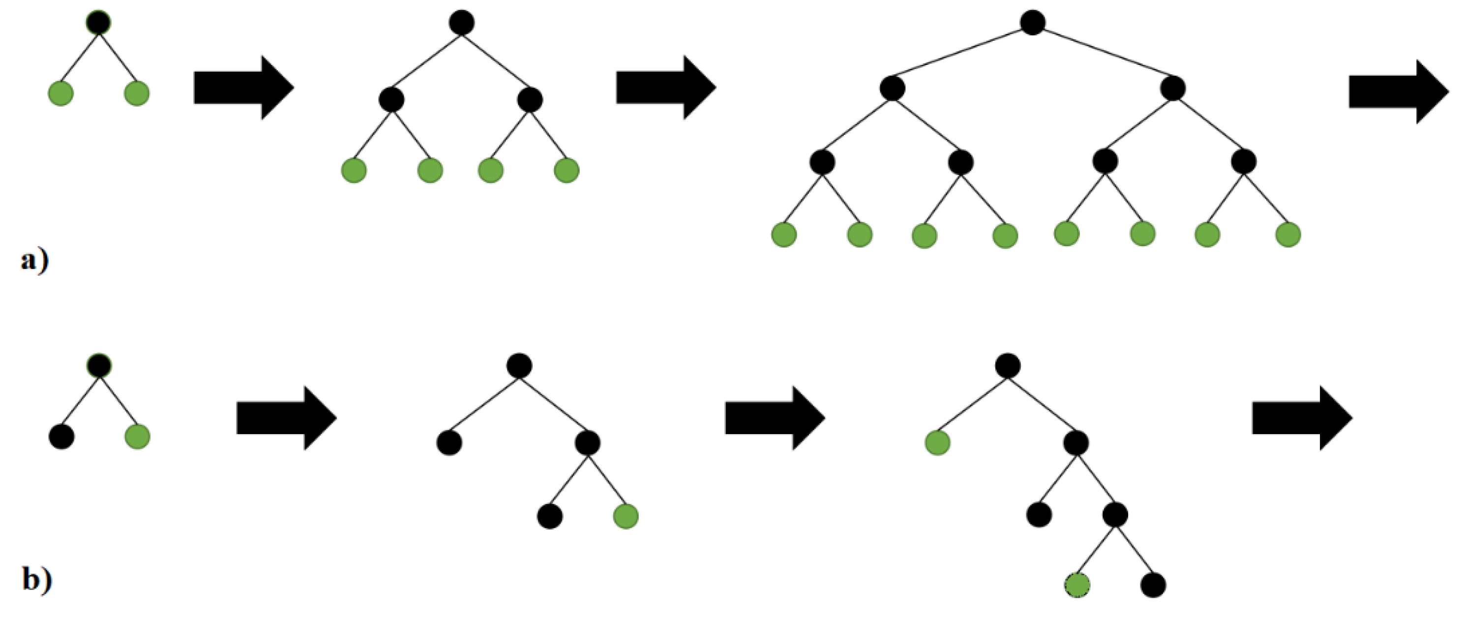
8]. The primary difference is that LightGBM decision trees are constructed in a leaf-wise manner, rather than evaluating all previous leaves for each new leaf (
Figure 4a,b). The attributes are grouped and sorted into bins, known as the histogram implementation. LightGBM offers several benefits, including faster training speed, higher accuracy, as well as the ability to handle large scale data and support GPU learning.
The focus of CatBoost is on categorical columns through the use of permutation methods, target-based statistics, and one_hot_max_size (OHMS). By using a greedy technique at each new split of the current tree, CatBoost has the capability to address the exponential growth of feature combinations. The steps described below are employed by CatBoost for each feature with more categories than the OHMS (an input parameter):
To randomly divide the records into subsets,
To convert the labels to integer numbers,
To transform the categorical features to numerical features, as follows:
Where
totalCount denotes the number of previous objects,
countInClass represents the number of ones in the target for a specific categorical feature, and the starting parameters specify
prior [
44,
45,
46].
4. Handling Imbalanced Data
Imbalanced data is a prevalent problem in data mining. For instance, in binary classifications, the number of instances in the majority class may be significantly higher than the number of instances in the minority class. As a result, the ratio of instances in the minority class to instances in the majority class (imbalanced ratio) may vary from 1:2 to 1:1000. The dataset used in this study is imbalanced, with the distribution of majority class (non-churned) instances being six times that of the minority class (churned) instances. This characteristic of the data leads to the construction of a biased classifier that has high accuracy for the majority class (non-churned) but low accuracy for the minority class (churned). Several sampling methods have been proposed to address this issue. Sampling techniques are applied to imbalanced data to alter the class distribution and create balanced data. Generally, sampling techniques are divided into two categories: undersampling and oversampling [
47].
A. Sampling Techniques
Synthetic Minority Over-Sampling Technique (SMOTE) [
48] is an oversampling technique that aims to balance the data by replicating instances of the minority class and is widely utilized to address this issue.
Tomek Links is an undersampling method, and an extension to the Condensed Nearest Neighbor (CNN) method, proposed by Ivan Tomek (in his 1976 paper titled "Two modifications of CNN") [
49]. The Tomek links method identifies pairs of examples (each from a different class) that have the minimum Euclidean distance to each other.
Edited Nearest Neighbors (ENN) is another undersampling method, proposed by Wilson (in his 1972 paper titled "Asymptotic Properties of Nearest Neighbor Rules Using Edited Data") [
50]. This method computes the three nearest neighbors for each instance in the dataset. If the instance belongs to the majority class and is misclassified by its three nearest neighbors, then it is removed from the dataset. Alternatively, if the instance belongs to the minority class and is misclassified by its three nearest neighbors, then the three majority-class instances are removed.
Applying just one undersampling or oversampling method to the training data can effectively handle imbalanced data, but to achieve the best results, it is advisable to use combination techniques. In this study, to address imbalanced data, we use two of the most popular combinations of sampling techniques, such as the combination of SMOTE and Tomek Links, and the combination of SMOTE and ENN.
B. Training and Validation Process
For evaluating our classifiers, we employ the k-fold cross-validation technique. However, there is a limitation when using this technique with imbalanced data. The issue is that, with this technique, the data is split into k-folds with a uniform probability distribution, and in imbalanced data, some folds may have no or few examples from the minority class. To address this issue, we can use a stratified sampling technique when performing train-test split or k-fold cross-validation. Using stratification ensures that each split of the data has an equal number of instances from the minority class.
We utilize an out-of-sample testing approach to evaluate the performance of the models. This approach demonstrates the performance of the models on unseen data that was not used to train the models.
When working with imbalanced data, it is essential to up-sample or down-sample only after splitting the data into a train and test sets (and validate if desired). If the dataset is up-sampled prior to splitting it into test and train, it is likely that the model experiences data leakage. This way, we may wrongly assume that our machine learning model is performing well. After building a machine learning model, it is recommended to test the metric on the not-up-sampled train dataset. When the metric is tested on the not-up-sampled dataset, the model's performance can be more realistically estimated compared to when it is tested on the up-sampled dataset.
5. Evaluation Metrics
We employ two types of metrics to evaluate our models. 1) Threshold metrics: These metrics are designed to minimize the error rate and assist in calculating the exact number of predicted values that do not match the actual values. 2) Ranking metrics: These metrics are designed to evaluate the effectiveness of classifiers at separating classes. These metrics require classifiers to predict a probability or a score of class membership. By applying different thresholds, we can test the effectiveness of classifiers, and those classifiers that maintain a good score across a range of thresholds will have better class separation and, as a result, will have a higher rank.
A. Threshold Metrics
Normally, we use the standard accuracy metric (equation 6) for measuring the performance of ML models. However, for imbalanced data, classification ML models may achieve high accuracy, as this metric only considers the majority class. In an imbalanced dataset, instances of the minority class (churned) are rare, and thus, True Positives (TP) do not have a significant impact on the standard accuracy metric. This metric, therefore, cannot accurately represent the performance of the models. For example, if the model correctly predicts all data points in the majority class (non-churned), it will result in high True Negatives (TN) and a high standard of accuracy, without accurately predicting anything about the minority class (churned). In the case of imbalanced data, this metric is not sufficient as a benchmark criterion measure [
51]. Therefore, other metrics such as recall, precision, and F-measure are commonly used to evaluate the performance of ML models in minority classes, and can be extracted from the confusion matrix, as shown in
Table 1.
The confusion matrix helps us to understand the performance of ML models by showing which class is being predicted correctly and which one is being predicted incorrectly.
In
Table 1, TP and FP stand for True Positive and False Positive, and FN and TN stand for False Negative and True Negative, respectively. Precision, Recall, and Accuracy can be calculated using the following formulas:
But Precision and Recall are not sufficient for evaluating the accuracy of the mentioned methods, since they do not provide enough information and can be misleading. Therefore, we usually use the F-measure metric as a single metric to evaluate the accuracy of our models. F-measure is a combination of Precision and Recall metrics and balances both precision and recall and provides a single metric that represents the overall performance of the model. F-measure is defined as follows:
The more the value of the F-measure is closer to 1, the better combination of Precision and Recall is achieved by the model [
52].
B. Ranking Metrics
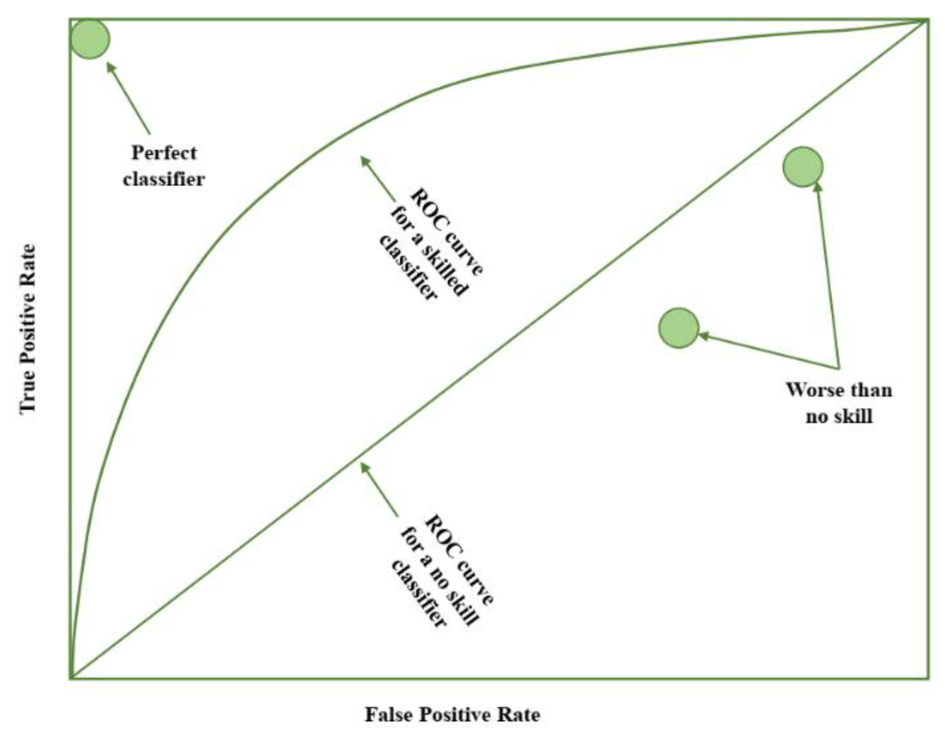
In the field of churn prediction, the Receiver Operating Characteristic (ROC) Curve is widely recognized as a prominent ranking metric for evaluating the performance of classifiers. This metric enables the assessment of a classifier's ability to differentiate between classes by providing a visual representation of the true positive rate and false positive rate of predicted values, as calculated under various threshold values.
The true positive rate (recall or sensitivity) is calculated as follows:
And the false positive rate is calculated as follows:
Each point on the plot represents a prediction made by the model, with the curve being formed by connecting all points. A line running diagonally from the bottom left to the top right on the plot represents a model with no skill, and any point located below this line represents a model that performs worse than one with no skill. Conversely, a point in the top left corner of the plot symbolizes a perfect model.
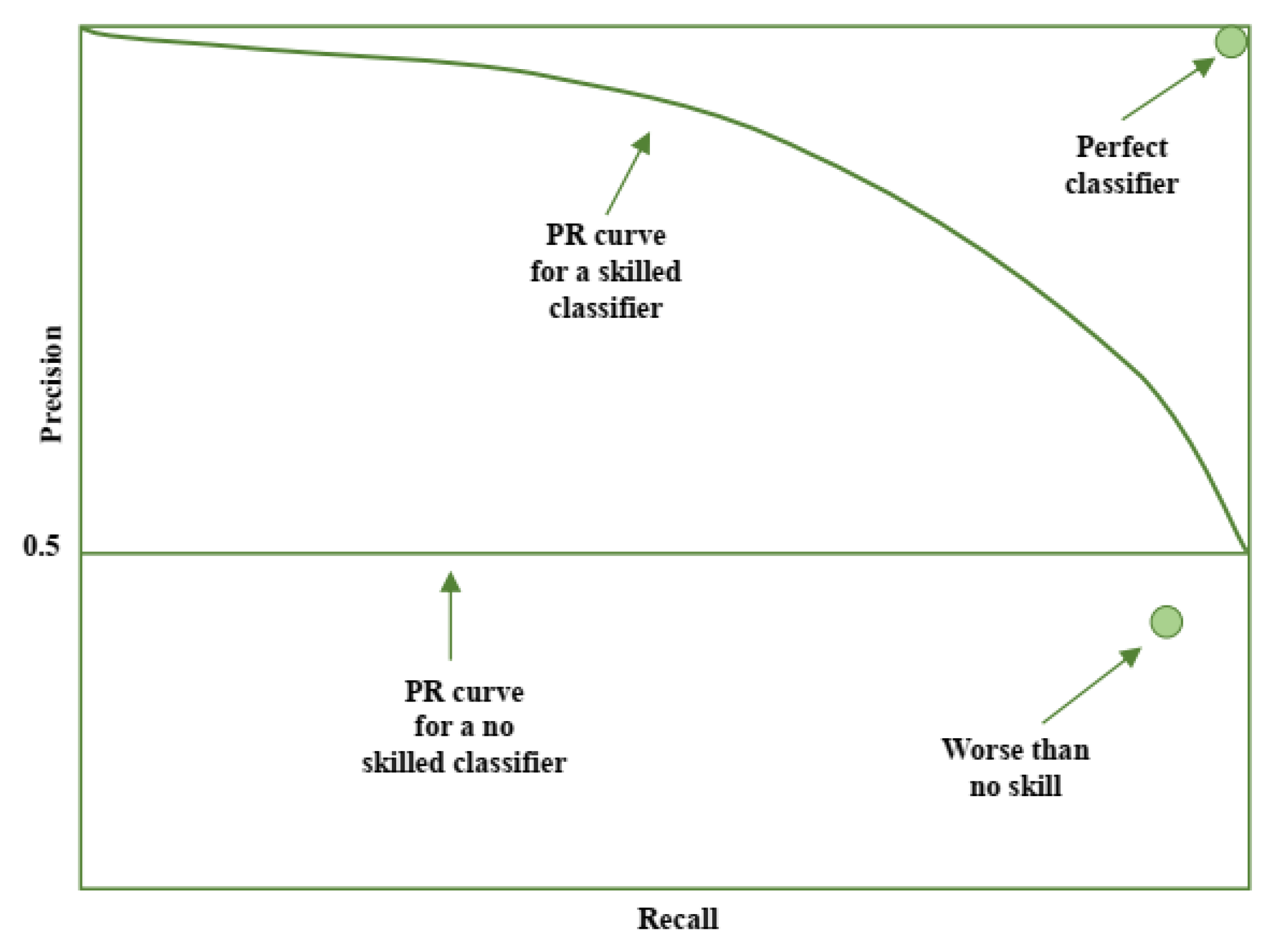
The area under the ROC curve can be calculated and utilized as a single score to evaluate the performance of models. A classifier with no skill has a score of 0.5, and a perfect classifier has a score of 1.0. However, it should be noted that the ROC curve can be effective for classification problems with a low imbalanced ratio, and can be optimistic for classification problems with a high imbalanced ratio. In such cases, the precision-recall curve is a more appropriate metric, as it focuses on the performance of the classifier on the minority class.
Figure 6.
The Precision-Recall curve.
Figure 6.
The Precision-Recall curve.
The ROC curve is a widely used method for evaluating the performance of machine learning models. The ROC curve plots the true positive rate against the false positive rate at various threshold settings, with each point on the curve representing a predicted value by the model.
A horizontal line on the plot signifies a model with no skill, while points below the diagonal line indicate a model that performs worse than random chance. Conversely, a point located in the top left quadrant of the plot represents a model with perfect performance.
In datasets with a balanced distribution of positive and negative examples, the horizontal line on the ROC plot is typically set at 0.5. However, when the dataset is imbalanced, such as with an imbalanced ratio of 1:10, the horizontal line is adjusted to 0.1 to reflect the imbalanced nature of the data.
In addition to the ROC curve, the area under the ROC curve (AUC) is also a commonly used metric for evaluating the performance of machine learning models. The AUC provides a single score for comparing the performance of different models. In cases where the dataset has a high imbalanced ratio, the Precision-Recall AUC (PR AUC) may be more informative as it specifically focuses on the performance of the minority class. However, if the imbalanced ratio of the dataset is not excessively high, such as the dataset utilized in this study, the use of PR AUC may not be necessary for evaluation.
In this paper, we employ a comprehensive set of metrics to evaluate the performance of machine learning models, including Recall, Precision, F1-score, and Receiver Operating Characteristic (ROC) AUC. These metrics provide a comprehensive evaluation of the model's performance, including its ability to accurately identify positive examples, balance false positives and false negatives, and handle imbalanced datasets.
Unlike the standard accuracy metric, ROC AUC places a particular emphasis on the performance of the minority class, and the accurate prediction of minority class instances is central to its calculation. This is particularly useful in situations where the dataset is imbalanced, as it ensures that the model's performance is evaluated fairly and in a way that takes into account the specific characteristics of the data.
C. ROC AUC Benchmark
It is clear that a ROC Area Under the Curve (AUC) of 100% represents the optimal performance that a machine learning model can achieve, as it indicates that all instances of the positive class (e.g. churns in the case of customer retention) are ranked higher in risk than all instances of the negative class (e.g. non-churns). However, it is highly unlikely that any model will achieve this level of performance in real-world problems.
As such, when comparing the performance of different machine learning models using ROC AUC, it is necessary to have a benchmark to determine whether the model's performance is acceptable. The ROC AUC ranges from 50% to 100%, with 50% being equivalent to random guessing and 100% representing perfect performance. As can be seen in
Table 2, the worst possible AUC is 50%, which is similar to the result of a coin flip for prediction.
6. Simulation
A. Simulation Setup
The primary objective of this study is to evaluate and compare the performance of several popular classification techniques in solving the problem of customer churn prediction. The classifiers under examination include Decision Tree, Logistic Regression, Random Forest, Support Vector Machine, XGBoost, LightGBM, and CatBoost. To achieve this goal, simulations were conducted using the Python programming language and various libraries such as Pandas, NumPy, and Scikit-learn.
A real-world dataset was used for this study, which was obtained from Kaggle, and is outlined in
Table 3. The training dataset consists of 20 attributes and 4250 instances, while the testing dataset has 20 attributes and 750 instances. The training dataset features a churn rate of 14.1% and an active subscriber rate of 85.9%. The performance of the models was evaluated using a variety of metrics, including precision, recall, F-measure, and ROC AUC as defined previously. After undergoing pre-processing steps such as handling categorical variables, feature selection, and removing outliers, these metrics were evaluated using both the training and testing datasets. Additionally, the SMOTE technique was used to handle imbalanced data and the effect on the performance of the models was examined.
7. Simulation Results
In this study, we evaluate the performance of several machine learning models (Decision Tree, Logistic Regression, Artificial Neural Network, Support Vector Machine, Random Forest, XGBoost, LightGBM, and CatBoost) on unseen data using a range of metrics including precision, recall, F1-Score, Receiver Operating Characteristic (ROC) Area Under the Curve (AUC), and Precision-Recall (PR) AUC. The evaluation is carried out on the testing dataset to assess the generalization ability of the models and to determine their performance on unseen data.
A. Applying Feature Selection
After undergoing several pre-processing steps such as handling categorical features and feature selection, the aforementioned models were applied to the data and their performance was evaluated. The results of this evaluation are presented in
Table 4, with the highest values highlighted in bold.
As depicted in
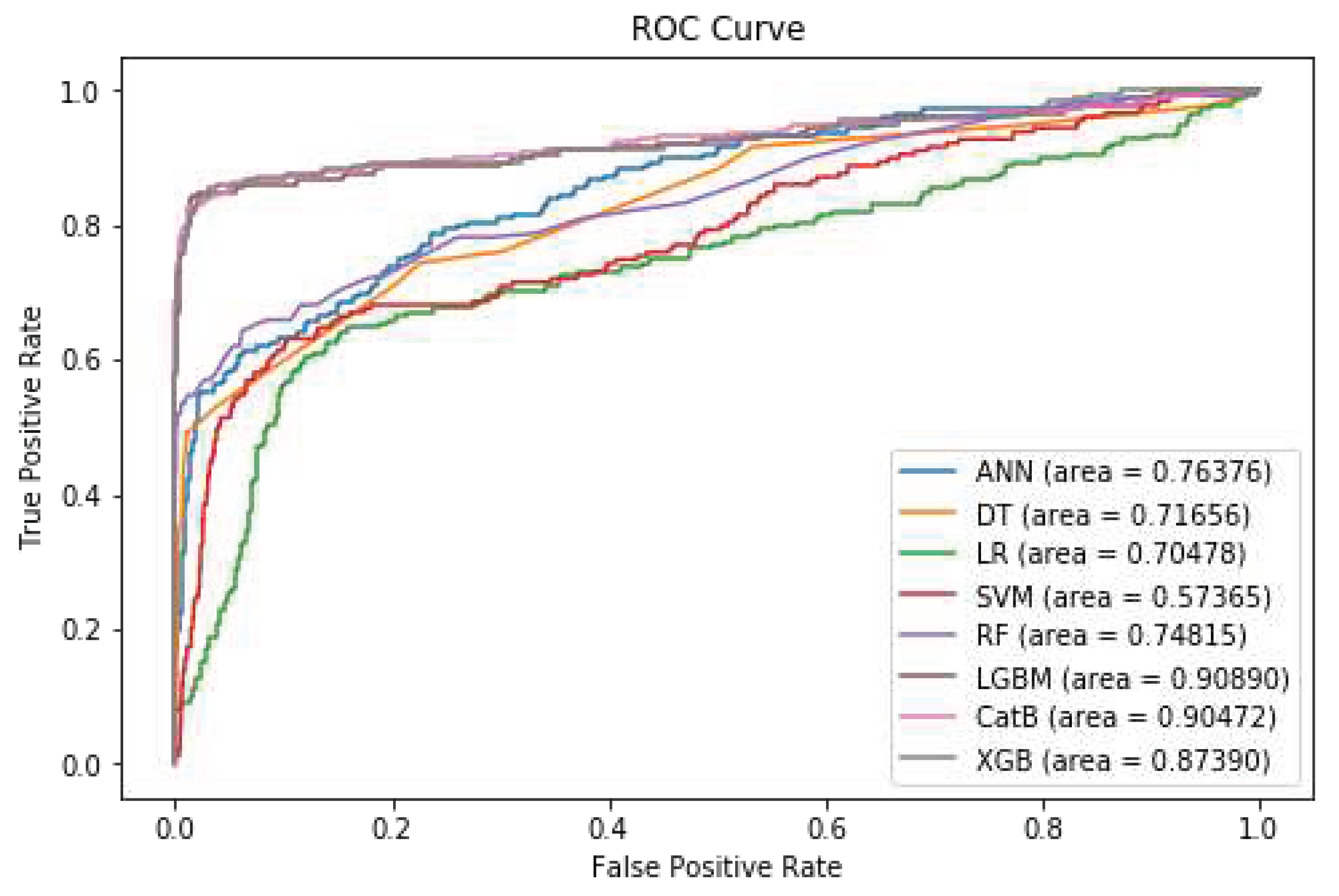
Table 4, the Random Forest and XGBoost models exhibit superior performance in terms of precision compared to other machine learning algorithms. However, in terms of recall, F1-Score, and ROC AUC, the LightGBM model outperforms the other methods.
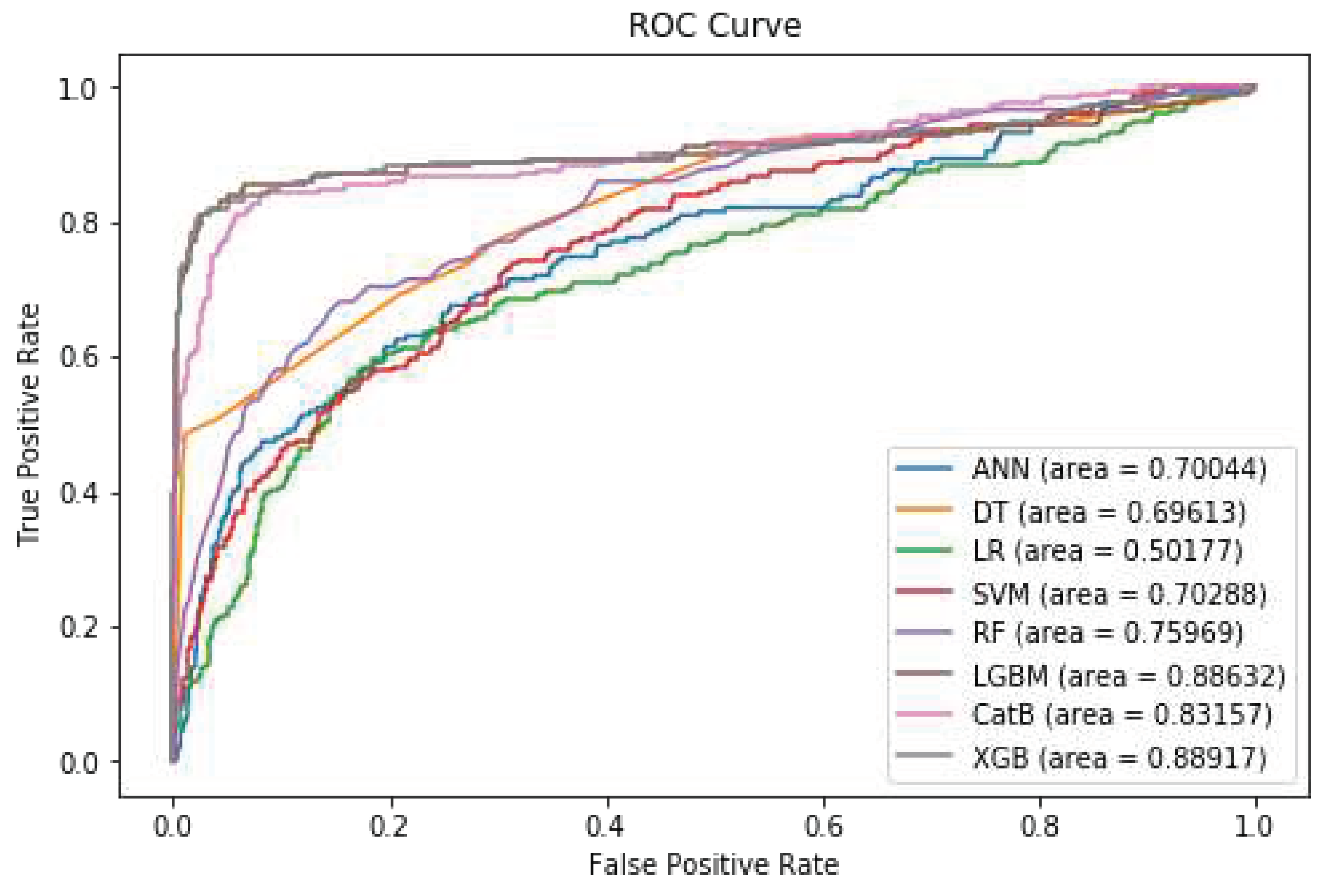
Figure 7 shows the diagram of the ROC Curve for the different models after feature selection.
B. Applying SMOTE
To address the issue of class imbalance in the training data, where the number of instances of class-0 is 3652 and the number of instances of class-1 is 598, we have applied the SMOTE technique to the training dataset. This technique was used to create synthetic instances of the minority class in order to achieve a balanced training dataset. As a result of the application of SMOTE, the number of instances for both class-0 and class-1 is now equal to 2125.
As
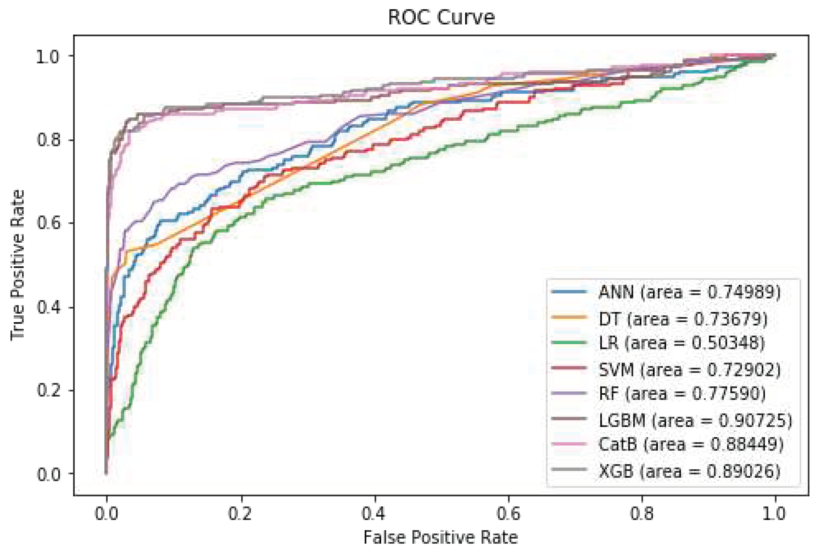
Table 5 shows, LightGBM and XGBoost outperform other ML techniques in all evaluation metrics.
Figure 8 shows the diagram of the ROC Curve for the different models after applying SMOTE.
C. Applying SMOTE with Tomek Links
As previously discussed in Section IV, the Tomek Links method is an undersampling technique that is used to identify pairs of examples, where each example belongs to a different class, that have the minimum Euclidean distance to each other. Additionally, as noted in the section, it is beneficial to utilize a combination of both oversampling and undersampling techniques to achieve optimal results. The results of the evaluation metrics for the various models after applying the SMOTE technique in conjunction with Tomek Links are presented in
Table 6. As evidenced by the table, both LightGBM and XGBoost outperform the other machine learning methods and demonstrate slightly improved results when compared to utilizing SMOTE alone, as shown in
Table 5.
Figure 9 shows the diagram of the ROC Curve for the different models after applying SMOTE with Tomek Links.
D. Applying SMOTE with ENN
As previously discussed in Section IV, the ENN method is employed to compute the three nearest neighbors for each instance within the dataset. In instances where the sample belongs to the majority class and is misclassified by its three nearest neighbors, the instance is removed from the dataset. Conversely, if the instance belongs to the minority class and is misclassified by its three nearest neighbors, the three majority class instances are removed. Furthermore, as previously stated, it has been shown to be beneficial to utilize a combination of undersampling and oversampling techniques in order to achieve optimal results.
Table 7 illustrates the evaluation metrics for the various models following the application of the SMOTE technique in conjunction with the ENN method. The results indicate that LightGBM and XGBoost models outperform other machine learning techniques in all evaluation metrics once more.
Figure 10 shows the diagram of the ROC Curve for the different models after applying SMOTE with Tomek Links.
E. Applying OPTUNA Hyperparameter Optimizer
Takuya Akiba et al. (2019) [
53] introduced Optuna, an open-source Python library for hyperparameter optimization. Optuna aims to balance the pruning and sampling algorithms through the execution of various techniques, such as the Tree-Structured of Parzen Estimator (TPE) [
54,
55] for independent parameter sampling, Covariance Matrix Adaptation (CMA) [
56], and Gaussian Processes (GP) [
55] for relational parameter sampling. The library also utilizes a variant of the Asynchronous Successive Halving (ASHA) algorithm [
57] to prune search spaces. In this study, we applied the Optuna library to the popular machine learning models, CatBoost, XGBoost, and LightGBM. The results, as presented in
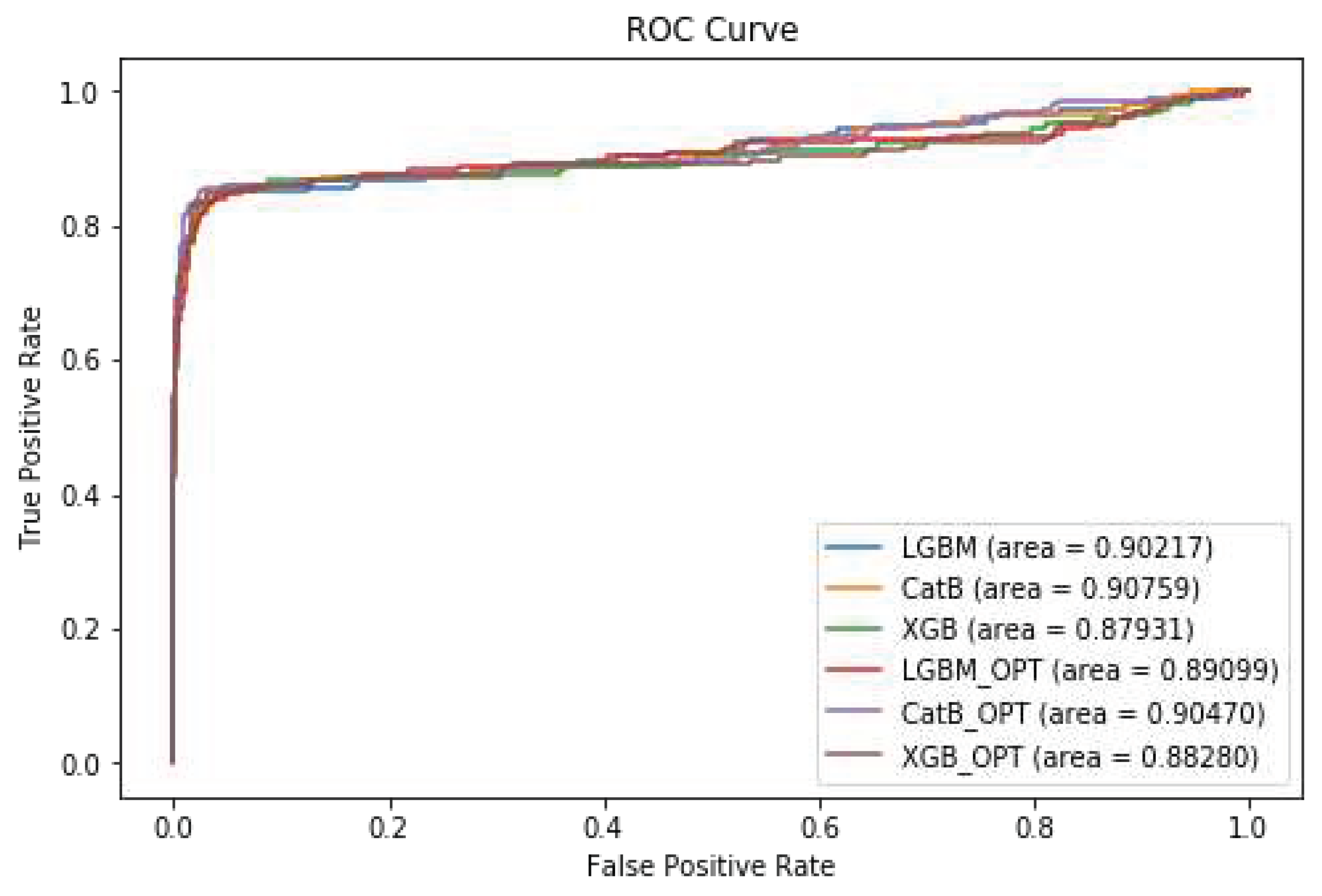
Table 8, indicate that CatBoost outperforms XGBoost and LightGBM when utilizing Optuna for hyperparameter optimization.
Figure 11 shows the diagram of the ROC Curve for the different models after applying OPTUNA hyperparameter tuning.
8. Conclusion
In this study, we employed various machine learning (ML) models, including Artificial Neural Networks, Decision Trees, Support Vector Machines, Random Forests, Logistic Regression, and three modern gradient boosting techniques, namely XGBoost, LightGBM, and CatBoost, to predict customer churn in the telecommunications industry using a real-world imbalanced dataset. We evaluated the impact of different sampling techniques, such as SMOTE, SMOTE with Tomek Links, and SMOTE with ENN, to handle the imbalanced data. We then assessed the performance of the ML models using various metrics, including Precision, Recall, F1-score, and Receiver Operating Characteristic Area Under the Curve (ROC AUC). Finally, we utilized the Optuna hyperparameter optimization technique on CatBoost, LightGBM, and XGBoost to determine the effect of optimization on the performance of the models. We compared the results of all the steps and presented them in tabular form.
The simulation results demonstrate the performance of different models on unseen data. LightGBM and XGBoost consistently exhibit superior performance across various evaluation metrics, including precision, recall, F1-Score, and ROC AUC. The performance of these models is further improved when applying techniques such as SMOTE with Tomek Links or SMOTE with ENN to handle imbalanced data. Additionally, the use of Optuna hyperparameter optimization for CatBoost, XGBoost, and LightGBM models shows further improvements in performance.
In future work, several avenues can be explored. Firstly, other machine learning techniques, such as deep learning models like Long Short-Term Memory (LSTM) or Transformer-based models, can be evaluated for churn prediction. These models have shown promise in various domains and may provide further insights into churn behavior. Secondly, we suggest exploring the use of the AdaSyn technique to handle imbalanced data and compare the results. Lastly, we recommend applying the above techniques to a highly imbalanced dataset to evaluate their performance in such conditions. Furthermore, employing the learning curve method to determine whether the models are overfitting could also be a valuable avenue of research.
Author Contributions
Writing and original draft preparation, M.I.; supervision, review, and editing, H.R.A. All authors have read and agreed to the published version of the manuscript.
Funding
This research received no external funding.
Institutional Review Board Statement
Not applicable.
Informed Consent Statement
Not applicable.
Data Availability Statement
Not applicable.
Conflicts of Interest
The authors declare no conflict of interest.
References
- The Chartered Institute of Marketing. Cost of Customer Acquisition versus Customer Retention. 2010.
- Eichinger, F.; Nauck, D.D.; Klawonn, F. Sequence mining for customer behaviour predictions in telecommunications. In Proceedings of the Workshop on Practical Data Mining at ECML/PKDD; 2006; pp. 3–10. [Google Scholar]
- Prasad, U.D.; Madhavi, S. Prediction of churn behaviour of bank customers using data mining tools. Indian J. Market. 2011, 42, 25–30. [Google Scholar]
- Keramati, A.; Ghaneei, H.; Mirmohammadi, S.M. Developing a prediction model for customer churn from electronic banking services using data mining. Financial Innov. 2016, 2, 10. [Google Scholar] [CrossRef]
- Scriney, Michael, Dongyun Nie, and Mark Roantree. Predicting customer churn for insurance data. In International Conference on Big Data Analytics and Knowledge Discovery; Springer: Cham, 2020. [Google Scholar] [CrossRef]
- De Caigny, Arno, Kristof Coussement, and Koen W. De Bock. A new hybrid classification algorithm for customer churn prediction based on logistic regression and decision trees. European Journal of Operational Research 2018, 269, 760–772. [Google Scholar] [CrossRef]
- Kim, K.; Jun, C.-H.; Lee, J. Improved churn prediction in telecommunication industry by analyzing a large network. Expert Syst. Appl. 2014, 41, 6575–6584. [Google Scholar] [CrossRef]
- Ahmad, A.K.; Jafar, A.; Aljoumaa, K. Customer churn prediction in telecom using machine learning in big data platform. J. Big Data 2019, 6, 28. [Google Scholar] [CrossRef]
- De Caigny, Arno, Kristof Coussement, and Koen W. De Bock. A new hybrid classification algorithm for customer churn prediction based on logistic regression and decision trees. European Journal of Operational Research 2018, 269, 760–772. [Google Scholar] [CrossRef]
- Jadhav, R.J.; Pawar, U.T. Churn prediction in telecommunication using data mining technology. IJACSA Edit. 2011, 2, 17–19. [Google Scholar]
- Radosavljevik, D.; van der Putten, P.; Larsen, K.K. The impact of experimental setup in prepaid churn prediction for mobile telecommunications: what to predict, for whom and does the customer experience matter? Trans MLDM 2010, 3, 80–99. [Google Scholar]
- Richter, Y.; Yom-Tov, E.; Slonim, N. Predicting customer churn in mobile networks through analysis of social groups. SDM, vol. 2010, SIAM, 2010, pp. 732–741.
- Amin, A.; Shah, B.; Khattak, A.M.; Moreira, F.J.L.; Ali, G.; Rocha, A.; Anwar, S. Cross-company customer churn prediction in telecommunication: A comparison of data transformation methods. Int. J. Inf. Manag. 2018, 46, 304–319. [Google Scholar] [CrossRef]
- Tsiptsis, K.; Chorianopoulos, A. Data Mining Techniques in CRM: Inside Customer Segmentation; John Wiley & Sons, 2011. [Google Scholar]
- Joudaki, Majid, et al. Presenting a New Approach for Predicting and Preventing Active/Deliberate Customer Churn in Telecommunication Industry. In Proceedings of the International Conference on Security and Management (SAM). The Steering Committee of the World Congress in Computer Science, Computer Engineering and Applied Computing (WorldComp); 2011. [Google Scholar]
- Amin, A.; Al-Obeidat, F.; Shah, B.; Adnan, A.; Loo, J.; Anwar, S. Customer churn prediction in telecommunication industry using data certainty. J. Bus. Res. 2019, 94, 290–301. [Google Scholar] [CrossRef]
- Shaaban, E.; Helmy, Y.; Khedr, A.; Nasr, M. A proposed churn prediction model. J. Eng. Res. Appl. 2012, 2, 693–697. [Google Scholar]
- Khan, Y.; Shafiq, S.; Naeem, A.; Ahmed, S.; Safwan, N.; Hussain, S. Customers Churn Prediction using Artificial Neural Networks (ANN) in Telecom Industry. Int. J. Adv. Comput. Sci. Appl. 2019, 10. [Google Scholar] [CrossRef]
- Ho, Tin Kam. Random decision forests. Proceedings of 3rd international conference on document analysis and recognition; 1995; 1. [Google Scholar] [CrossRef]
- Breiman, Leo. Random forests. Machine learning 2001, 45, 5–32. [Google Scholar] [CrossRef]
- Amin, A.; Shehzad, S.; Khan, C.; Ali, I.; Anwar, S. Churn prediction in telecommunication industry using rough set approach. In New Trends in Computational Collective Intelligence; Springer, 2015; pp. 83–95. [Google Scholar]
- Witten, I.H.; Frank, E.; Hall, M.A.; Pal, C.J. Data Mining : Practical Machine Learning Tools and Techniques; Elsevier Science & Technology: San Francisco, 2016. [Google Scholar]
- Kumar, A.; Jain, M. Ensemble Learning for AI Developers: Learn Bagging, Stacking, and Boosting Methods with Use Cases, Apress, 2020.
- van Wezel, M.; Potharst, R. Improved customer choice predictions using ensemble methods. Eur. J. Oper. Res. 2007, 181, 436–452. [Google Scholar] [CrossRef]
- Ullah, I.; Raza, B.; Malik, A.K.; Imran, M.; Islam, S.U.; Kim, S.W. A Churn Prediction Model Using Random Forest: Analysis of Machine Learning Techniques for Churn Prediction and Factor Identification in Telecom Sector. IEEE Access 2019, 7, 60134–60149. [Google Scholar] [CrossRef]
- Lalwani, P.; Mishra, M.K.; Chadha, J.S.; Sethi, P. Customer churn prediction system: a machine learning approach. Computing 2021, 104, 271–294. [Google Scholar] [CrossRef]
- Tarekegn, A.; Ricceri, F.; Costa, G.; Ferracin, E.; Giacobini, M. Predictive Modeling for Frailty Conditions in Elderly People: Machine Learning Approaches. Psychopharmacol. 2020, 8, e16678. [Google Scholar] [CrossRef]
- Ahmed, M.; Afzal, H.; Siddiqi, I.; Amjad, M.F.; Khurshid, K. Exploring nested ensemble learners using overproduction and choose approach for churn prediction in telecom industry. Neural Comput. Appl. 2018, 32, 3237–3251. [Google Scholar] [CrossRef]
- Boser, B.E.; Guyon, I.M.; Vapnik, V.N. A training algorithm for optimal margin classifiers. In Proceedings of the Fifth Annual Workshop on Computational Learning Theory. ACM; 1992; pp. 144–152. [Google Scholar]
- Hur, Y.; Lim, S. Customer churning prediction using support vector machines in online auto insurance service. In Advances in Neural Networks” – ISNN 2005; Springer, 2005; pp. 928–933. [Google Scholar]
- Lee, S.J.; Siau, K. A review of data mining techniques. Ind. Manag. Data Syst. 2001, 101, 41–46. [Google Scholar] [CrossRef]
- Mazhari, N. Imani, M., Joudaki, M. and Ghelichpour, A.,"An overview of classification and its algorithms" 3rd Data Mining Conference (IDMC'09): Tehran, 2009.
- Linoff, G.S.; Berry, M.J. Data Mining Techniques: For Marketing, Sales, and Customer Relationship Management; John Wiley & Sons, 2011.
- Zhou, Z.-H. Ensemble Methods - Foundations and Algorithms; Taylor & Francis group, LLC: 2012.
- Kumar, A.; Jain, M. , Ensemble Learning for AI Developers: Learn Bagging, Stacking, and Boosting Methods with Use Cases, Apress, 2020.
- Witten, I.H.; Frank, E.; Hall, M.A.; Pal, C.J. Data Mining: Practical Machine Learning Tools and Techniques; Elsevier Science & Technology: San Francisco, 2016. [Google Scholar]
- Karlberg, J.; Axen, M. Binary Classification for Predicting Customer Churn; Umeå University: Umeå, 2020. [Google Scholar]
- Windridge, D.; Nagarajan, R. "Quantum Bootstrap Aggregation. In Proceedings of the International Symposium on Quantum Interaction; 2017. [Google Scholar] [CrossRef]
- Wang, J.C.; Hastie, T. Boosted Varying-Coefficient Regression Models for Product Demand Prediction. J. Comput. Graph. Stat. 2014, 23, 361–382. [Google Scholar] [CrossRef]
- Al Daoud, E. Intrusion Detection Using a New Particle Swarm Method and Support Vector Machines. World Academy of Science, Engineering and Technology 2013, 77, 59–62. [Google Scholar]
- Al Daoud, E.; Turabieh, H. New empirical nonparametric kernels for support vector machine classification. Appl. Soft Comput. 2013, 13, 1759–1765. [Google Scholar] [CrossRef]
- Al Daoud, E. An Efficient Algorithm for Finding a Fuzzy Rough Set Reduct Using an Improved Harmony Search. Int. J. Mod. Educ. Comput. Sci. (IJMECS) 2015, 7, 16–23. [Google Scholar] [CrossRef]
- Zhang, Y.; Haghani, A. A gradient boosting method to improve travel time prediction. Transp. Res. Part C: Emerg. Technol. 2015, 58, 308–324. [Google Scholar] [CrossRef]
- Dorogush, A.; Ershov, V.; Gulin, A. CatBoost: gradient boosting with categorical features support. NIPS 2017. [Google Scholar]
- Qi, M.; Guolin, K.; Taifeng, W.; Wei, C.; Qiwei, Y.; Weidong, M.; TieYan, L. A Communication-Efficient Parallel Algorithm for Decision Tree. Advances in Neural Information Processing Systems 2016, 29, 1279–1287. [Google Scholar]
- Klein, A.; Falkner, S.; Bartels, S.; Hennig, P.; Hutter, F. Fast Bayesian optimization of machine learning hyperparameters on large datasets. Proceedings of Machine Learning Research PMLR; 2017; 54, pp. 528–536. [Google Scholar]
- 47. Kubat, Miroslav, and Stan Matwin. Addressing the curse of imbalanced training sets: one-sided selection. Icml.
- Chawla, Nitesh V. , et al. SMOTE: synthetic minority over-sampling technique. Journal of artificial intelligence research 2002, 16, 321–357. [Google Scholar] [CrossRef]
- Tomek, I. Two Modifications of CNN. IEEE Trans. Syst. Man, Cybern. 1976, SMC-6, 769–772. [Google Scholar] [CrossRef]
- Wilson, D.L. Asymptotic Properties of Nearest Neighbor Rules Using Edited Data. IEEE Trans. Syst. Man Cybern. 1972, 2, 408–421. [Google Scholar] [CrossRef]
- Tyagi, S.; Mittal, S. , "Sampling Approaches for Imbalanced Data Classification Problem in Machine Learning," in Proceedings of ICRIC 2019, 2020. [CrossRef]
- Fawcett, T. An Introduction to ROC analysis. Pattern Recogn. Lett. 2006, 27, 861–874. [Google Scholar] [CrossRef]
- Akiba, Takuya, et al. Optuna: A next-generation hyperparameter optimization framework. In Proceedings of the 25th ACM SIGKDD international conference on knowledge discovery & data mining. 2019.
- Bergstra, James, Daniel Yamins, and David Cox. Making a science of model search: Hyperparameter optimization in hundreds of dimensions for vision architectures. In Proceedings of The 30th International Conference on Machine Learning. 2013.
- 55. Bergstra, James S., et al. Algorithms for hyper-parameter optimization. Advances in Neural Information Processing Systems.
- Hansen, N.; Ostermeier, A. Completely Derandomized Self-Adaptation in Evolution Strategies. Evol. Comput. 2001, 9, 159–195. [Google Scholar] [CrossRef] [PubMed]
- Li, Liam, et al. A system for massively parallel hyperparameter tuning. Proceedings of Machine Learning and Systems 2020, 2, 230–246. [Google Scholar]
|
Disclaimer/Publisher’s Note: The statements, opinions and data contained in all publications are solely those of the individual author(s) and contributor(s) and not of MDPI and/or the editor(s). MDPI and/or the editor(s) disclaim responsibility for any injury to people or property resulting from any ideas, methods, instructions or products referred to in the content. |
© 2023 by the authors. Licensee MDPI, Basel, Switzerland. This article is an open access article distributed under the terms and conditions of the Creative Commons Attribution (CC BY) license (http://creativecommons.org/licenses/by/4.0/).
