1. Introduction
The implementation of Customer Relationship Management (CRM) is a strategic approach to managing and enhancing relationships between businesses and their customers. CRM is a tool employed to gain deeper insights into the requirements and behaviors of consumers, specifically end users, with the aim of fostering a more robust and meaningful relationship with them. Through the utilization of CRM, businesses can establish an infrastructure that fosters long-term and loyal customers. This concept is relevant across various industries, such as banking [
1,
2,
3,
4], insurance companies [
5], and telecommunications [
6,
7,
8,
9,
10,
11,
12,
13,
14,
15], to name a few.
The telecommunications sector assumes a prominent role as a leading industry in revenue generation and a crucial driver of socioeconomic advancement in numerous countries globally. It is estimated that this sector incurs expenditures of approximately 4.7 trillion dollars annually [
1,
2]. Within the sector, there exists a high degree of competition among companies, driven by their pursuit of augmenting revenue streams and expanding market influence through the acquisition of an expanded customer base. A key objective of CRM is customer retention, as studies have demonstrated that the cost of acquiring new customers can be 20 times higher than retaining existing ones [
1]. Therefore, maintaining existing customers in the telecommunications industry is crucial for increasing revenue and reducing marketing and advertising costs.
The telecommunications sector is grappling with the substantial issue of customer attrition, commonly referred to as churn. This escalating issue has prompted service providers to shift their emphasis from acquiring new customers to retaining existing ones, considering the significant costs associated with customer acquisition. In recent years, service providers have been progressively emphasizing the establishment of enduring relationships with their customers. Consequently, these providers uphold CRM databases wherein every customer-specific interaction is systematically documented [
5]. CRM databases serve as valuable resources for proactively predicting and addressing customer requirements by leveraging a combination of business processes and machine learning (ML) methodologies to analyze and understand customer behavior.
The primary goal of ML models is to predict and categorize customers into one of two groups: churn or non-churn, representing a binary classification problem. As a result, it is imperative for businesses to develop practical tools to achieve this goal. In recent years, various ML methods have been proposed for constructing a churn model, including Artificial Neural Networks (ANN) [
8,
9,
16,
17,
18], Decision Trees (DT) [
8,
9,
11,
13,
16,
17], Random Forests (RF) [
19,
20], Logistic Regression (LR) [
9,
13], Support Vector Machines (SVM) [
17], and Rough Set Approach [
21], among others.
In the following, an overview is provided of the most frequently utilized techniques for addressing the issue of churn prediction, including Artificial Neural Network, Decision Trees, Support Vector Machines, Random Forests, Logistic Regression, and three advanced gradient boosting techniques, namely eXtreme Gradient Boosting (XGBoost), Categorical Boosting (CatBoost) and Light Gradient Boosting Machine (LightGBM).
Ensemble techniques [
22], specifically boosting and bagging algorithms, have become the prevalent choice for addressing classification problems [
23,
24], particularly in the realm of churn prediction [
25,
26], due to their demonstrated high effectiveness. While many studies have explored the field of churn prediction, our research distinguishes itself by offering a comprehensive examination of how machine learning techniques, imbalanced data, and predictive accuracy intersect.
We carefully investigate a wide range of machine learning algorithms, along with innovative data sampling methods and precise hyperparameter optimization techniques. The objective is to offer subscription-based companies a comprehensive framework for effectively tackling the complex task of predicting customer churn. In the current data-centric business environment, the relevance of this study is not only significant but also imperative. It equips subscription-based businesses with the tools to retain customers, optimize revenue, and develop lasting relationships with their customers in the face of evolving industry dynamics. This study makes several significant contributions, including:
- 1-
Providing a comprehensive definition of binary classification machine learning techniques tailored for imbalanced data.
- 2-
Conducting an extensive review of diverse sampling techniques designed to address imbalanced data.
- 3-
Offering a detailed account of the training and validation procedures within imbalanced domains.
- 4-
Explaining the key evaluation metrics that are well-suited for imbalanced data scenarios.
- 5-
Employing various machine learning models and conducting a thorough assessment, comparing their performance using commonly employed metrics across three distinct phases: after applying feature selection, after applying SMOTE, after applying SMOTE combined with Tomek Links, after applying SMOTE combined with ENN, and after applying Optuna hyperparameter tuning.
Table 1, below, shows a summary of the important acronyms used throughout this paper.
The remainder of the paper is organized as follows:
Section 2 presents an introduction to classification machine learning techniques,
Section 3 delves into the examination of sampling methods,
Section 4 explains the training and validation process,
Section 5 defines evaluation metrics, simulation results are presented in
Section 6, and the paper concludes in
Section 7.
2. Classification Machine Learning Techniques
2.1. Artificial Neural Network
Artificial Neural Network (ANN) is a widely employed technique for addressing complex issues such as the churn prediction problem [
27]. ANNs are structures composed of interconnected units that are modeled after the human brain. They can be utilized with various learning algorithms to enhance the machine learning process and can take both hardware and software forms. One of the most widely utilized models is the Multi-Layer Perceptron, which is trained using the Back-Propagation Network (BPN) algorithm. Research has demonstrated that ANNs possess superior performance compared to Decision Trees (DTs) [
27], and have been shown to exhibit improved performance when compared to Logistic Regression (LR) and DTs in the context of churn prediction [
28].
2.2. Support Vector Machine
The technique of Support Vector Machine (SVM) was first introduced by authors in [
29]. It is classified as a supervised learning technique that utilizes learning algorithms to uncover latent patterns within data. A popular method for improving the performance of SVMs is the utilization of kernel functions [
8]. In addressing customer churn problems, SVM may exhibit superior performance in comparison to Artificial Neural Networks (ANNs) and Decision Trees (DTs) based on the specific characteristics of the data [
17,
30].
For this study, we utilize both the Gaussian Radial Basis kernel function (RBF-SVM) and the Polynomial kernel function (Poly-SVM) for the Support Vector Machine (SVM) technique. These kernel functions are among the various options available for use with SVM.
For two samples
and
, the RBF kernel is defined as follows:
where
can be the squared Euclidean distance, and
is a free parameter.
For two samples
and
, the d-degree polynomial kernel is defined as follows:
where
and
is the polynomial degree.
2.3. Decision Tree
A Decision Tree is a representation of all potential decision pathways in the form of a tree structure [
31,
32]. As Berry and Linoff stated, “a Decision Tree is a structure that can be used to divide up a large collection of records into successively smaller sets of records by applying a sequence of simple decision rules” [
33]. Though they may not be as efficient in uncovering complex patterns or detecting intricate relationships within data, DTs may be used to address the customer churn problem, depending on the characteristics of the data. In DTs, class labels are indicated by leaves, and the conjunctions between various features are represented by branches.
2.4. Logistic Regression
Logistic Regression (LR) is a classification method that falls under the category of probabilistic statistics. It can be employed to address the churn prediction problem by making predictions based on multiple predictor variables. In order to obtain high accuracy, which can sometimes be comparable to that of Decision Trees [
10], it is often beneficial to apply pre-processing and transformation techniques to the original data prior to utilizing LR.
2.5. Ensemble Learning
Ensemble learning is one of the widely utilized techniques in machine learning for combining the outputs of multiple learning models (often referred to as base learners) into a single classifier [
34]. In ensemble learning, it is possible to combine various weak machine learning models (base learners) to construct a stronger model with more accurate predictions [
35,
36]. Currently, ensemble learning methods are widely accepted as a standard choice for enhancing the accuracy of machine learning predictors [
35]. Bagging and boosting are two distinct types of ensemble learning techniques that can be utilized to improve the accuracy of machine learning predictors [
36].
2.5.1. Bagging
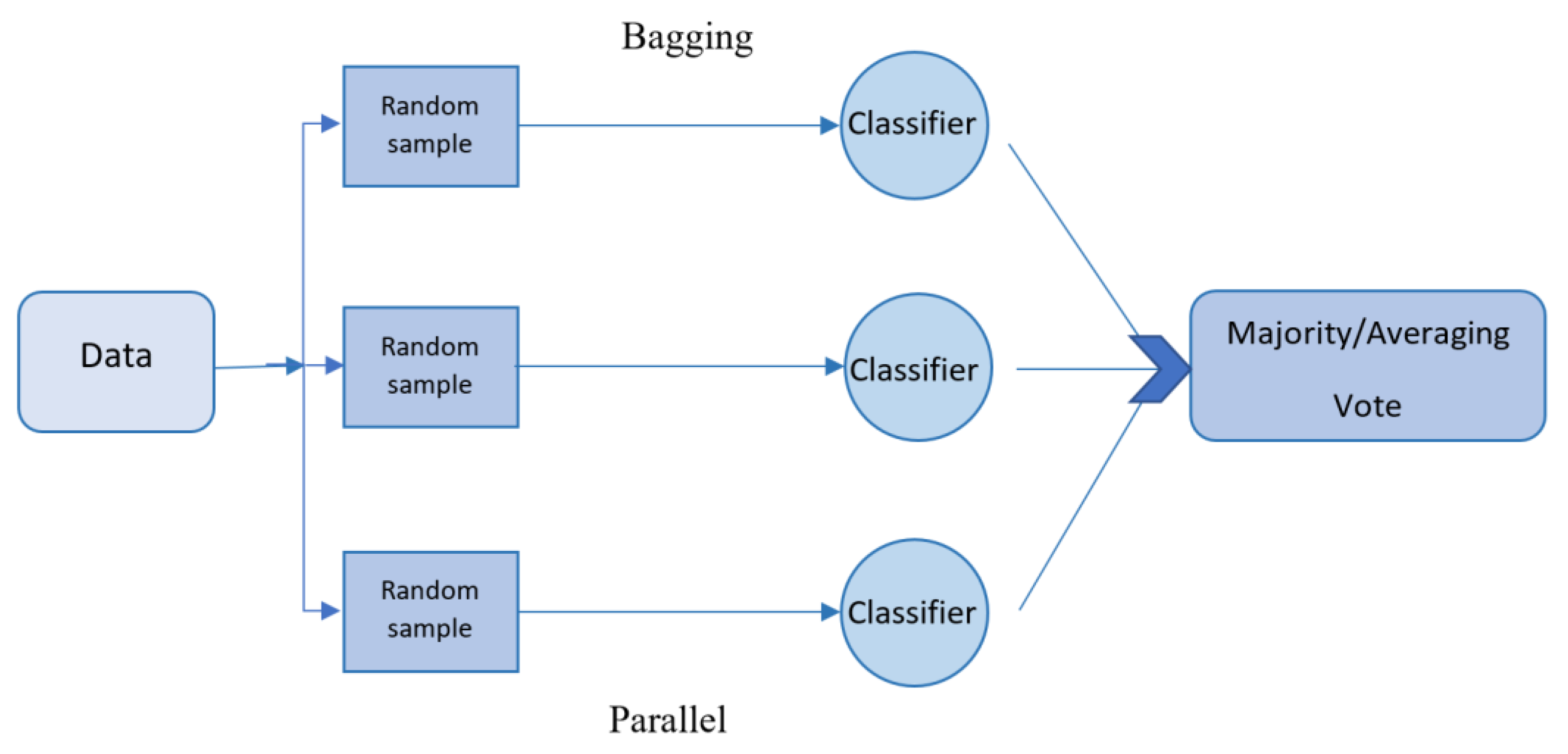
As depicted in
Figure 1, in the bagging technique, the training data is partitioned into multiple subset sets, and the model is trained on each subset. The final prediction is then obtained by combining all individual outputs through majority voting (in classification problems) or average voting (in regression problems) [
36,
37,
38].
2.5.1.1. Random Forest
The concept of Random Forest was first introduced by Ho in 1995 [
19] and has been the subject of ongoing improvement by various researchers. One notable advancement in this field was made by Leo Breiman in 2001 [
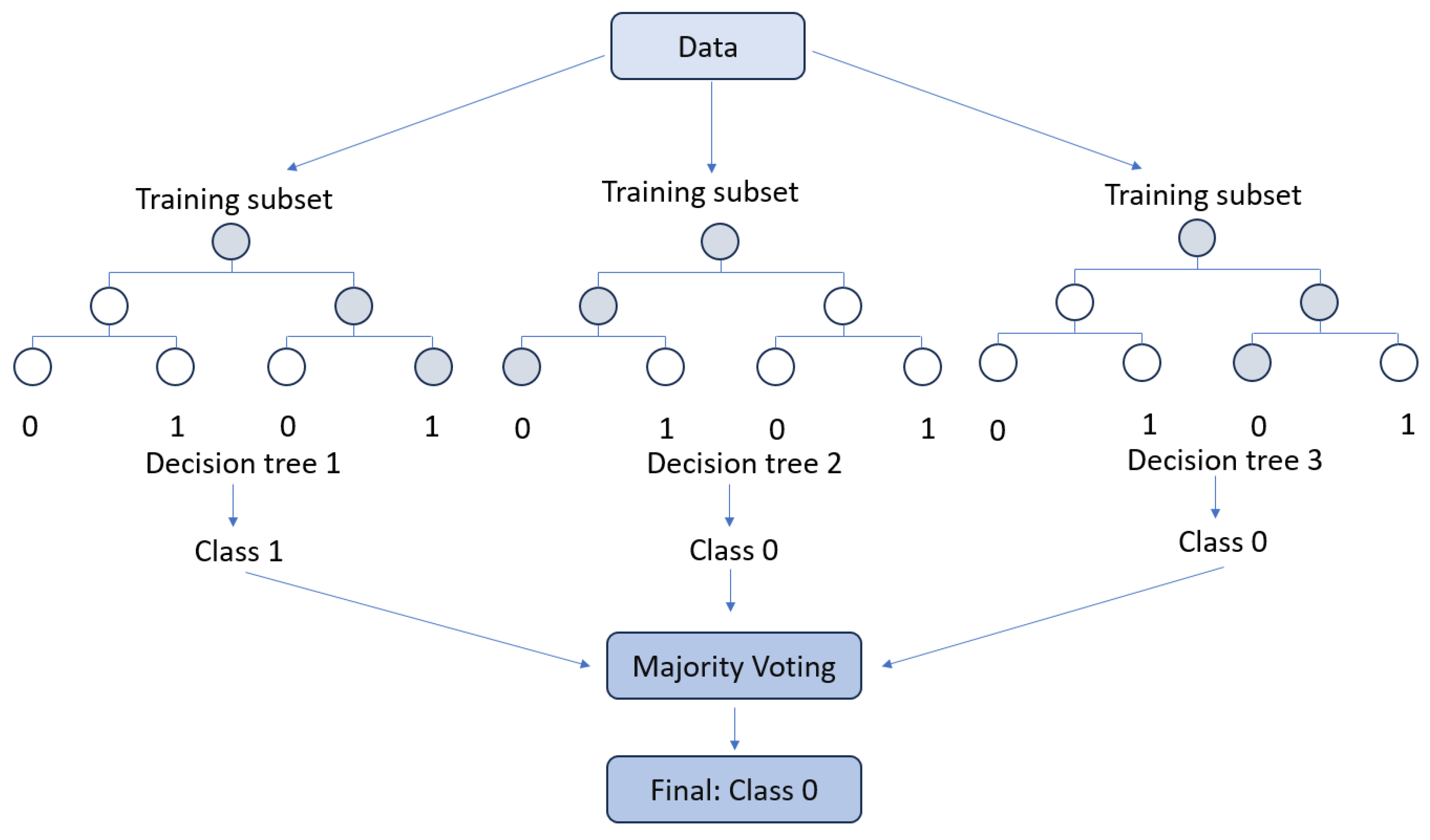
20]. Random Forests are an ensemble learning technique for classification tasks that employs a large number of Decision Trees in the training model. The output of Random Forests is a class that is selected by the majority of the trees, as shown in
Figure 2. In general, Random Forests exhibit superior performance compared to Decision Trees. However, the performance can be influenced by the characteristics of the data.
Random Forests utilize the bagging technique for their training algorithm. In greater detail, the Random Forests operate as follows: For a training set , bagging is repeated B times, and each iteration selects a random sample with a replacement from , and fits trees to the samples:
1- Sample training examples;
2- Train a classification tree (in the case of churn problems) on the samples .
After the training phase, Random Forests can predict unseen samples
by taking the majority vote from all the individual classification trees
.
2.5.2. Boosting
Boosting is another method for combining multiple base learners to construct a stronger model with more accurate predictions. The key distinction between bagging and boosting is that bagging uses a parallel approach to combine weak learners while boosting methods utilize a sequential approach to combine weak learners and derive the final prediction, as shown in
Figure 3. Like the bagging technique, boosting improves the performance of machine learning predictors, and in addition, it reduces the bias of the model [
36].
2.5.2.1. The Famous Trio: XGBoost, LightGBM, CatBoost
Recently, researchers have presented three effective gradient-based approaches using decision trees: CatBoost, LightGBM, and XGBoost. These new approaches have demonstrated successful applications in academia, industry, and competitive machine learning [
39]. Utilizing gradient boosting techniques, solutions can be constructed in a stagewise manner, and the over-fitting problem can be addressed through the optimization of loss functions. For example, given a loss function
and a custom base-learner
h(x, θ) (e.g., decision tree), the direct estimation of parameters can be challenging. Thus, an iterative model is proposed, which is updated at each iteration with the selection of a new base-learner function
h(x, θt), where the increment is directed by:
Hence, the hard optimization problem is substituted with the typical least-squares optimization problem:
The Friedman’s gradient boost algorithm is summarized by Algorithm 1.
| Algorithm 1 Gradient Boost |
|
After initiating the algorithm with a single leaf, the learning rate is optimized for each record and each node [
40,
41,
42]. The XGBoost method is a highly flexible, versatile, and scalable tool that has been developed to effectively utilize resources and overcome the limitations of previous gradient boosting methods. The primary distinction between other gradient boosting methods and XGBoost is that XGBoost utilizes a new regularization approach for controlling overfitting, making it more robust and efficient when the model is fine-tuned. To regularize this approach, a new term is added to the loss function as follows:
where
w represents the value of each leaf, Ω indicates the regularization function, and |δ| denotes the number of branches. A new gain function is used by XGBoost, as follows:
The
Gain represents the score of no new child case,
H indicates the score of the left child, and
G denotes the score of the right child [
43].
To decrease the implementation time, the LightGBM method was developed by a team from Microsoft in April 2017 [
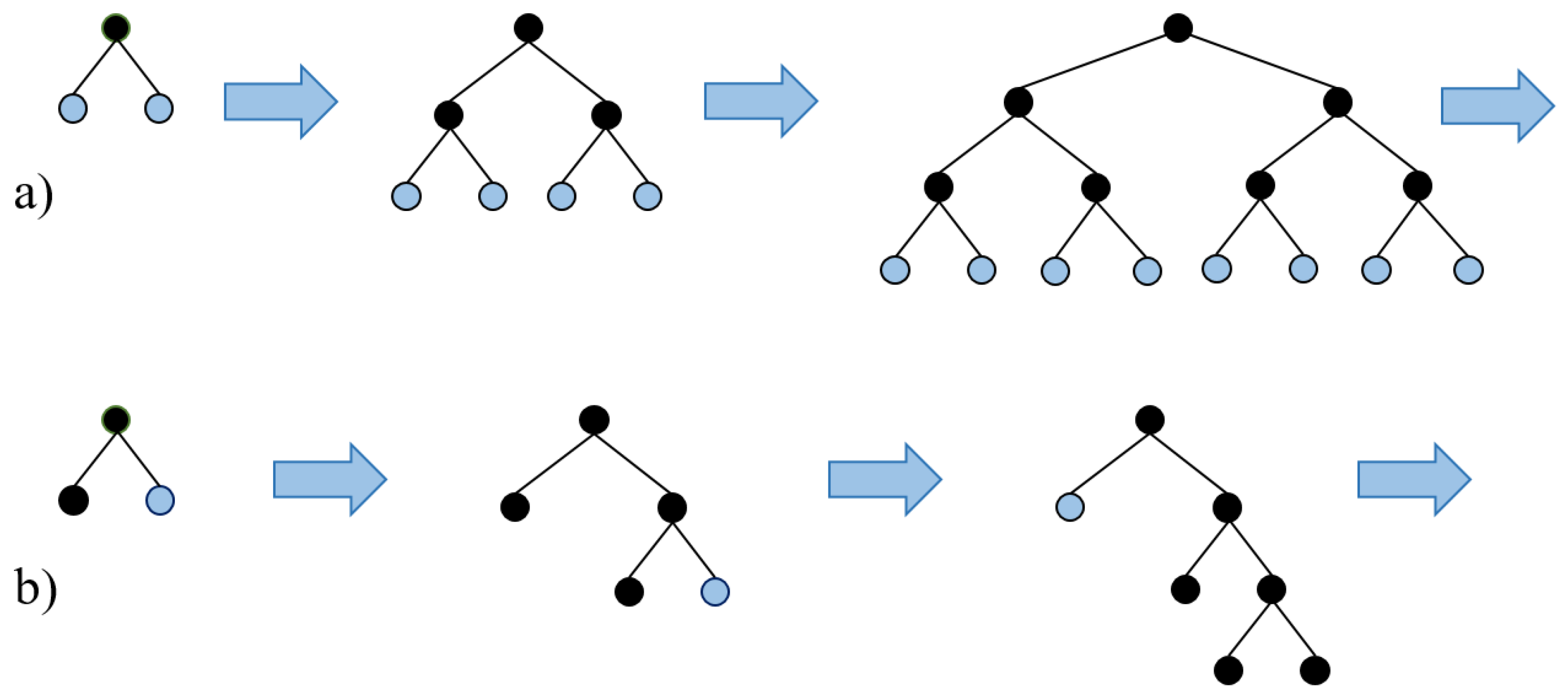
8]. The primary difference is that LightGBM decision trees are constructed in a leaf-wise manner, rather than evaluating all previous leaves for each new leaf (
Figure 4a and
Figure 4b). The attributes are grouped and sorted into bins, known as the histogram implementation. LightGBM offers several benefits, including faster training speed, higher accuracy, as well as the ability to handle large scale data and support GPU learning.
The focus of CatBoost is on categorical columns through the use of permutation methods, target-based statistics, and one_hot_max_size (OHMS). By using a greedy technique at each new split of the current tree, CatBoost has the capability to address the exponential growth of feature combinations. The steps described below are employed by CatBoost for each feature with more categories than the OHMS (an input parameter):
To randomly divide the records into subsets,
To convert the labels to integer numbers,
To transform the categorical features to numerical features, as follows:
where
totalCount denotes the number of previous objects,
countInClass represents the number of ones in the target for a specific categorical feature, and the starting parameters specify
prior [
44,
45,
46].
3. Handling Imbalanced Data
Imbalanced data is a prevalent problem in data mining. For instance, in binary classifications, the number of instances in the majority class may be significantly higher than the number of instances in the minority class. As a result, the ratio of instances in the minority class to instances in the majority class (imbalanced ratio) may vary from 1:2 to 1:1000. The dataset used in this study is imbalanced, with the distribution of majority class (non-churned) instances being six times that of the minority class (churned) instances [
58].
3.1. The Challenge of Imbalanced Data
While imbalanced datasets can skew overall model performance metrics towards the majority class, the more nuanced challenge lies in how specific algorithms inherently respond to this imbalance. For example, Support Vector Machines (SVM) inherently aim to find a hyperplane that delineates classes by maximizing the margin. However, with imbalanced datasets, the sheer volume of majority class instances can push this hyperplane in a way that does not genuinely represent the optimal boundary, especially from the perspective of the minority class.
In a similar vein, decision tree algorithms, which seek to achieve node purity through recursive partitioning, can end up favoring the majority class. In imbalanced contexts, the tree’s terminal nodes might predominantly represent the majority class, leading to compromised predictive accuracy for the minority instances.
Addressing these algorithmic biases necessitates approaches beyond mere accuracy metrics. Techniques like sampling, which adaptively adjust the class distribution, emerge as pivotal to mitigate such biases, ensuring that algorithms do not just superficially perform well but genuinely understand and predict minority class instances.
3.2. Sampling Techniques
This characteristic of the imbalanced data leads to the construction of a biased classifier that has high accuracy for the majority class (non-churned) but low accuracy for the minority class (churned). Several sampling methods have been proposed to address this issue. Sampling techniques are applied to imbalanced data to alter the class distribution and create balanced data. Generally, sampling techniques are divided into two categories: undersampling, where instances from the majority class are removed, and oversampling, where instances from the minority class are artificially increased [
47]. These methods aim to adjust the class distribution to enable the classifier to make better-informed decisions.
3.2.1. Synthetic Minority Over-Sampling Technique (SMOTE)
Synthetic Minority Over-Sampling Technique (SMOTE) [
48] is an oversampling technique that aims to balance the data by replicating instances of the minority class and is widely utilized to address this issue. Unlike simplistic methods that merely replicate minority instances, SMOTE innovatively crafts synthetic samples through an interpolation process between existing minority instances. This nuanced augmentation not only enhances the representation of the minority class but also fosters a more diverse and expansive decision boundary. Such an enriched decision space proves particularly beneficial for algorithms like Support Vector Machines (SVM), which are inherently sensitive to the distribution of instances in their modeling process.
3.2.2. Tomek Links
Tomek Links is an undersampling method and an extension to the Condensed Nearest Neighbor (CNN) method, proposed by Ivan Tomek (in his 1976 paper titled “Two modifications of CNN”) [
49]. The Tomek links method identifies pairs of examples (each from a different class) that have the minimum Euclidean distance from each other. By removing such instances, especially from the majority class, decision boundaries can become clearer and less prone to overlap. This enhanced delineation of decision spaces proves notably advantageous for classifiers, such as Decision Trees and k-Nearest Neighbors (k-NN), which rely heavily on a clear distinction between classes for optimal performance.
3.2.3. Edited Nearest Neighbors (ENN)
Edited Nearest Neighbors (ENN) is another undersampling method proposed by Wilson (in his 1972 paper titled “Asymptotic Properties of Nearest Neighbor Rules Using Edited Data”) [
50]. This method computes the three nearest neighbors for each instance in the dataset. If the instance belongs to the majority class and is misclassified by its three nearest neighbors, then it is removed from the dataset. Alternatively, if the instance belongs to the minority class and is misclassified by its three nearest neighbors, then the three majority-class instances are removed. This method often results in smoother decision boundaries, particularly benefiting algorithms sensitive to noisy data.
3.3. Combined Data Sampling Techniques
While individual sampling techniques can offer improvements, combining methods often yields superior results. This is because a combination captures the benefits of both oversampling and undersampling, refining decision boundaries and enhancing classifier robustness. In this study, to address imbalanced data, we use two of the most popular combinations of sampling techniques, such as the combination of SMOTE and Tomek Links and the combination of SMOTE and ENN.
4. Training and Validation Process
For evaluating our classifiers, we employ the k-fold cross-validation technique. However, there is a limitation when using this technique with imbalanced data. The issue is that, with this technique, the data is split into k-folds with a uniform probability distribution, and in imbalanced data, some folds may have no or few examples from the minority class. To address this issue, we can use a stratified sampling technique when performing train-test split or k-fold cross-validation. Using stratification ensures that each split of the data has an equal number of instances from the minority class.
We utilize an out-of-sample testing approach to evaluate the performance of the models. This approach demonstrates the performance of the models on unseen data that was not used to train the models.
When working with imbalanced data, it is essential to up-sample or down-sample only after splitting the data into train and test sets (and validate if desired). If the dataset is up-sampled prior to splitting it into test and train, it is likely that the model experiences data leakage. This way, we may wrongly assume that our machine learning model is performing well. After building a machine learning model, it is recommended to test the metric on the not-up-sampled train dataset. When the metric is tested on the not-up-sampled dataset, the model’s performance can be more realistically estimated compared to when it is tested on the up-sampled dataset.
5. Evaluation Metrics
We employ two types of metrics to evaluate our models. 1) Threshold metrics: These metrics are designed to minimize the error rate and assist in calculating the exact number of predicted values that do not match the actual values. 2) Ranking metrics: These metrics are designed to evaluate the effectiveness of classifiers in separating classes. These metrics require classifiers to predict a probability or a score of class membership. By applying different thresholds, we can test the effectiveness of classifiers, and those classifiers that maintain a good score across a range of thresholds will have better class separation and, as a result, will have a higher rank.
5.1. Threshold Metrics
Normally, we use the standard accuracy metric (equation 6) for measuring the performance of ML models. However, for imbalanced data, classification ML models may achieve high accuracy, as this metric only considers the majority class. In an imbalanced dataset, instances of the minority class (churned) are rare, and thus, True Positives (TP) do not have a significant impact on the standard accuracy metric. This metric, therefore, cannot accurately represent the performance of the models. For example, if the model correctly predicts all data points in the majority class (non-churned), it will result in high True Negatives (TN) and a high standard of accuracy without accurately predicting anything about the minority class (churned). In the case of imbalanced data, this metric is not sufficient as a benchmark criterion measure [
51]. Therefore, other metrics such as recall, precision, and F-measure are commonly used to evaluate the performance of ML models in minority classes and can be extracted from the confusion matrix, as shown in
Table 2.
The confusion matrix helps us to understand the performance of ML models by showing which class is being predicted correctly and which one is being predicted incorrectly.
In
Table 2, TP and FP stand for True Positive and False Positive, and FN and TN stand for False Negative and True Negative, respectively. Precision, Recall, and Accuracy can be calculated using the following formulas:
But Precision and Recall are not sufficient for evaluating the accuracy of the mentioned methods, since they do not provide enough information and can be misleading. Therefore, we usually use the F-measure metric as a single metric to evaluate the accuracy of our models. F-measure is a combination of Precision and Recall metrics and balances both precision and recall and provides a single metric that represents the overall performance of the model. F-measure is defined as follows:
The more the value of the F-measure is closer to 1, the better combination of Precision and Recall is achieved by the model [
52].
5.2. Ranking Metrics
In the field of churn prediction, the Receiver Operating Characteristic (ROC) Curve is widely recognized as a prominent ranking metric for evaluating the performance of classifiers. This metric enables the assessment of a classifier’s ability to differentiate between classes by providing a visual representation of the true positive rate and false positive rate of predicted values, as calculated under various threshold values.
The true positive rate (recall or sensitivity) is calculated as follows:
And the false positive rate is calculated as follows:
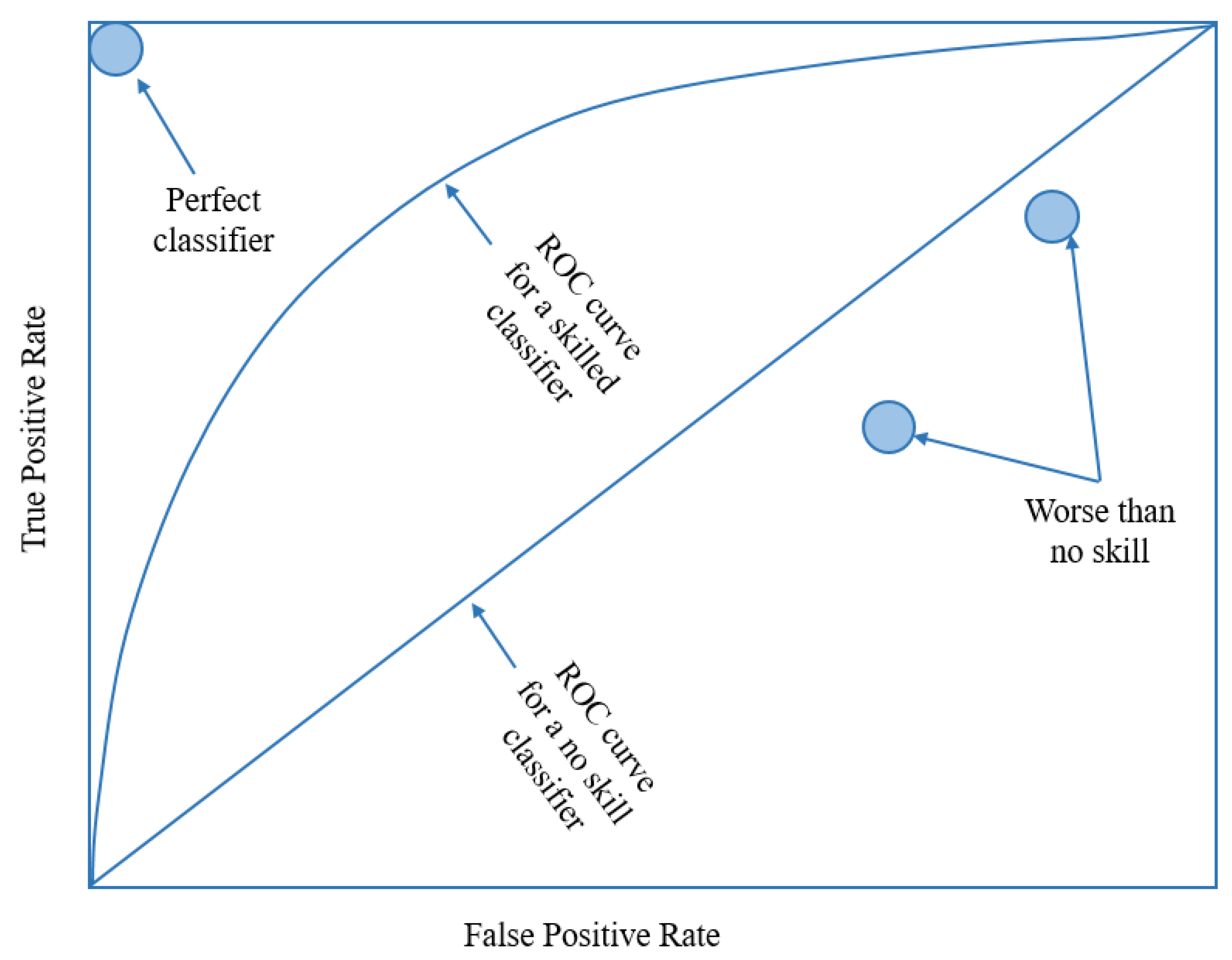
Each point on the plot represents a prediction made by the model, with the curve being formed by connecting all points. A line running diagonally from the bottom left to the top right on the plot represents a model with no skill, and any point located below this line represents a model that performs worse than one with no skill. Conversely, a point in the top left corner of the plot symbolizes a perfect model.
The area under the ROC curve can be calculated and utilized as a single score to evaluate the performance of models. A classifier with no skill has a score of 0.5, and a perfect classifier has a score of 1.0, as shown in
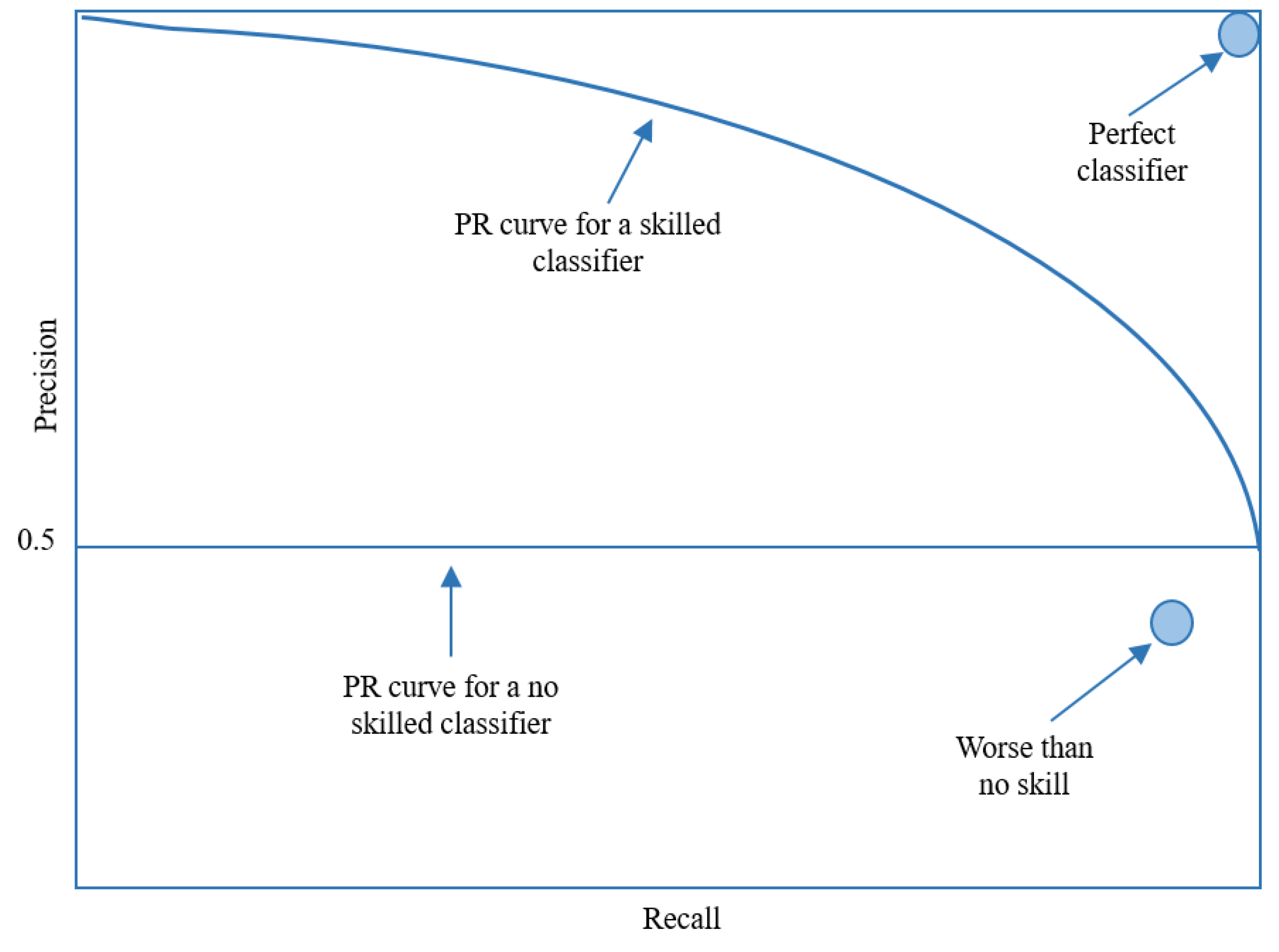
Figure 5. However, it should be noted that the ROC curve can be effective for classification problems with a low imbalanced ratio and can be optimistic for classification problems with a high imbalanced ratio. In such cases, the precision-recall curve is a more appropriate metric because it focuses on the performance of the classifier on the minority class, as depicted in
Figure 6.
The ROC curve is a widely used method for evaluating the performance of machine learning models. The ROC curve plots the true positive rate against the false positive rate at various threshold settings, with each point on the curve representing a predicted value by the model.
A horizontal line on the plot signifies a model with no skill, while points below the diagonal line indicate a model that performs worse than random chance. Conversely, a point located in the top left quadrant of the plot represents a model with perfect performance.
In datasets with a balanced distribution of positive and negative examples, the horizontal line on the ROC plot is typically set at 0.5. However, when the dataset is imbalanced, such as with an imbalanced ratio of 1:10, the horizontal line is adjusted to 0.1 to reflect the imbalanced nature of the data.
In addition to the ROC curve, the area under the ROC curve (AUC) is also a commonly used metric for evaluating the performance of machine learning models. The AUC provides a single score for comparing the performance of different models. In cases where the dataset has a high imbalanced ratio, the Precision-Recall AUC (PR AUC) may be more informative as it specifically focuses on the performance of the minority class. However, if the imbalanced ratio of the dataset is not excessively high, such as the dataset utilized in this study, the use of PR AUC may not be necessary for evaluation.
In this paper, we employ a comprehensive set of metrics to evaluate the performance of machine learning models, including Recall, Precision, F1-score, and Receiver Operating Characteristic (ROC) AUC. These metrics provide a comprehensive evaluation of the model’s performance, including its ability to accurately identify positive examples, balance false positives and false negatives, and handle imbalanced datasets.
Among these four metrics, we primarily focused on the F1-Score and ROC AUC metrics for the following reasons:
- ❖
F1-Score: Given the imbalance in our dataset, the F1-score is particularly useful as it does not inflate the performance of the model due to the high number of true negatives, which is a common issue with accuracy in such datasets.
- ❖
ROC AUC: Unlike the standard accuracy metric, ROC AUC places a particular emphasis on the performance of the minority class, and the accurate prediction of minority class instances is central to its calculation. This is particularly useful in situations where the dataset is imbalanced, as it ensures that the model’s performance is evaluated fairly. This metric is less sensitive to class imbalance and provides insight into the model’s ability to distinguish between classes, making it a robust measure for comparing the performance of different models.
5.3. ROC AUC benchmark
It is clear that a ROC Area Under the Curve (AUC) of 100% represents the optimal performance that a machine learning model can achieve, as it indicates that all instances of the positive class (e.g., churns in the case of customer retention) are ranked higher in risk than all instances of the negative class (e.g., non-churns). However, it is highly unlikely that any model will achieve this level of performance in real-world problems.
As such, when comparing the performance of different machine learning models using ROC AUC, it is necessary to have a benchmark to determine whether the model’s performance is acceptable. The ROC AUC ranges from 50% to 100%, with 50% being equivalent to random guessing and 100% representing perfect performance. As can be seen in
Table 3, the worst possible AUC is 50%, which is similar to the result of a coin flip for prediction. If the percentages are less than 50%, it indicates an issue with the model. Consider the worst-case scenario of obtaining a zero percent accuracy. While this might seem problematic, it actually means the model ranked all non-churn customers as higher risk than churn customers. Surprisingly, this result could be considered good because it implies your model can perfectly predict customer retention. However, most likely, there was an error in your model setup causing it to predict in the opposite direction.
In
Table 3, the categorization of the ROC AUC metric follows empirical norms and established methodologies within machine learning to yield a discernible evaluation of model efficacy. This discretization strategy is intended to furnish a pragmatic benchmark for evaluating churn prediction models, facilitating a straightforward appraisal for both researchers and practitioners.
6. Simulation
6.1. Simulation Setup
The primary objective of this study is to evaluate and compare the performance of several popular classification techniques in solving the problem of customer churn prediction. The classifiers under examination include Decision Tree, Logistic Regression, Random Forest, Support Vector Machine, XGBoost, LightGBM, and CatBoost. To achieve this goal, simulations were conducted using the Python programming language and various libraries such as Pandas, NumPy, and Scikit-learn.
A real-world dataset was used for this study, which was obtained from Kaggle and is outlined in
Table 4 [
57]. The training dataset consists of 20 attributes and 4250 instances, while the testing dataset has 20 attributes and 750 instances. The training dataset features a churn rate of 14.1% and an active subscriber rate of 85.9%. The performance of the models was evaluated using a variety of metrics, including precision, recall, F-measure, and ROC AUC as defined previously. After undergoing pre-processing steps such as handling categorical variables, feature selection, and removing outliers, these metrics were evaluated using both the training and testing datasets. Additionally, the SMOTE technique was used to handle imbalanced data, and the effect on the performance of the models was examined.
6.2. Simulation Results
In this study, we evaluate the performance of several machine learning models (Decision Tree, Logistic Regression, Artificial Neural Network, Support Vector Machine, Random Forest, XGBoost, LightGBM, and CatBoost) on unseen data using a range of metrics including precision, recall, F1-Score, Receiver Operating Characteristic (ROC) Area Under the Curve (AUC), and Precision-Recall (PR) AUC. The evaluation is carried out on the testing dataset to assess the generalization ability of the models and to determine their performance on unseen data.
6.2.1. After Pre-processing and Feature Selection
After undergoing several pre-processing steps, such as handling categorical features and feature selection, the aforementioned models were applied to the data, and their performance was evaluated. The results of this evaluation are presented in
Table 5, with the highest values highlighted in bold and marked with an asterisk.
As depicted in
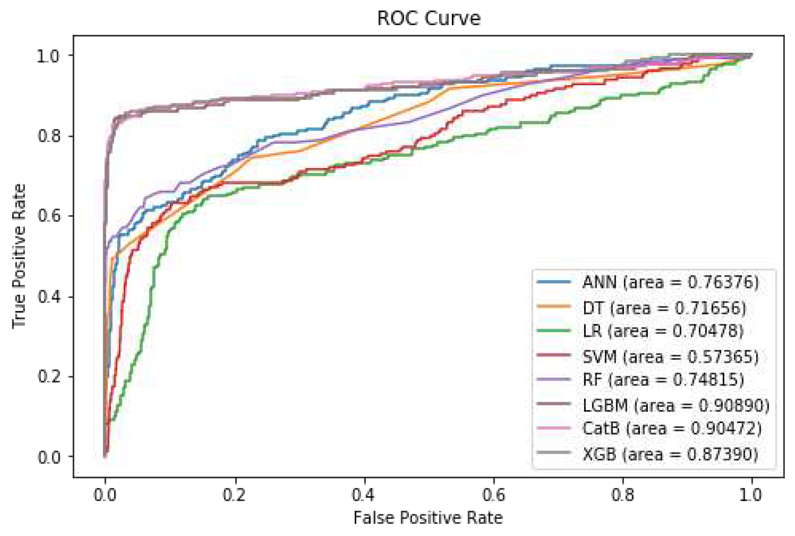
Table 5, the boosting models demonstrate superior performance, particularly in relation to F1-Score and ROC AUC metrics. Notably, LightGBM surpasses the performance of other methods, achieving an impressive F1-Score of 92% and an ROC AUC of 91%.
Figure 7 shows the diagram of the ROC Curve for the different models after pre-processing and feature selection.
6.2.2. Applying SMOTE
To address the issue of class imbalance in the training data, where the number of instances of class-0 is 3652, and the number of instances of class-1 is 598, we have applied the SMOTE technique to the training dataset. This technique was used to create synthetic instances of the minority class in order to achieve a balanced training dataset. As a result of the application of SMOTE, the number of instances for both class-0 and class-1 is now equal to 2125.
As
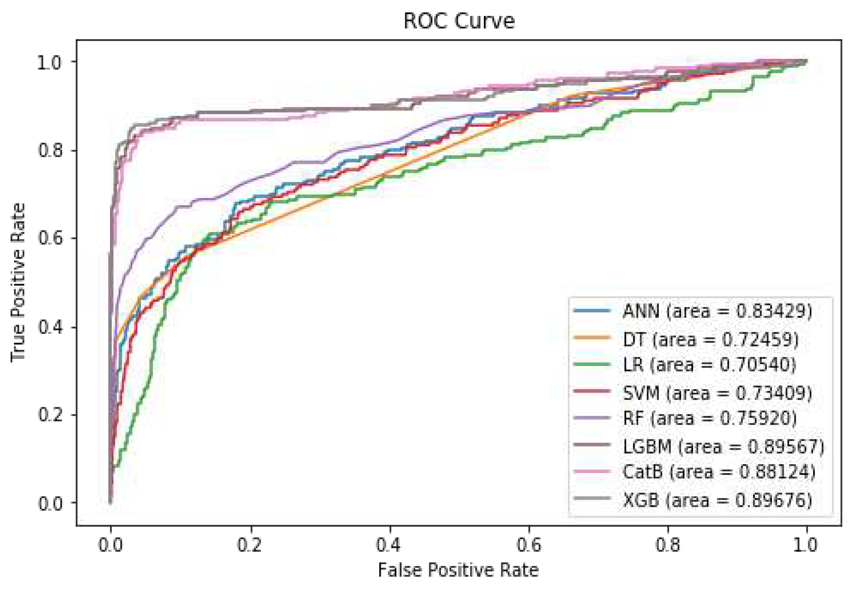
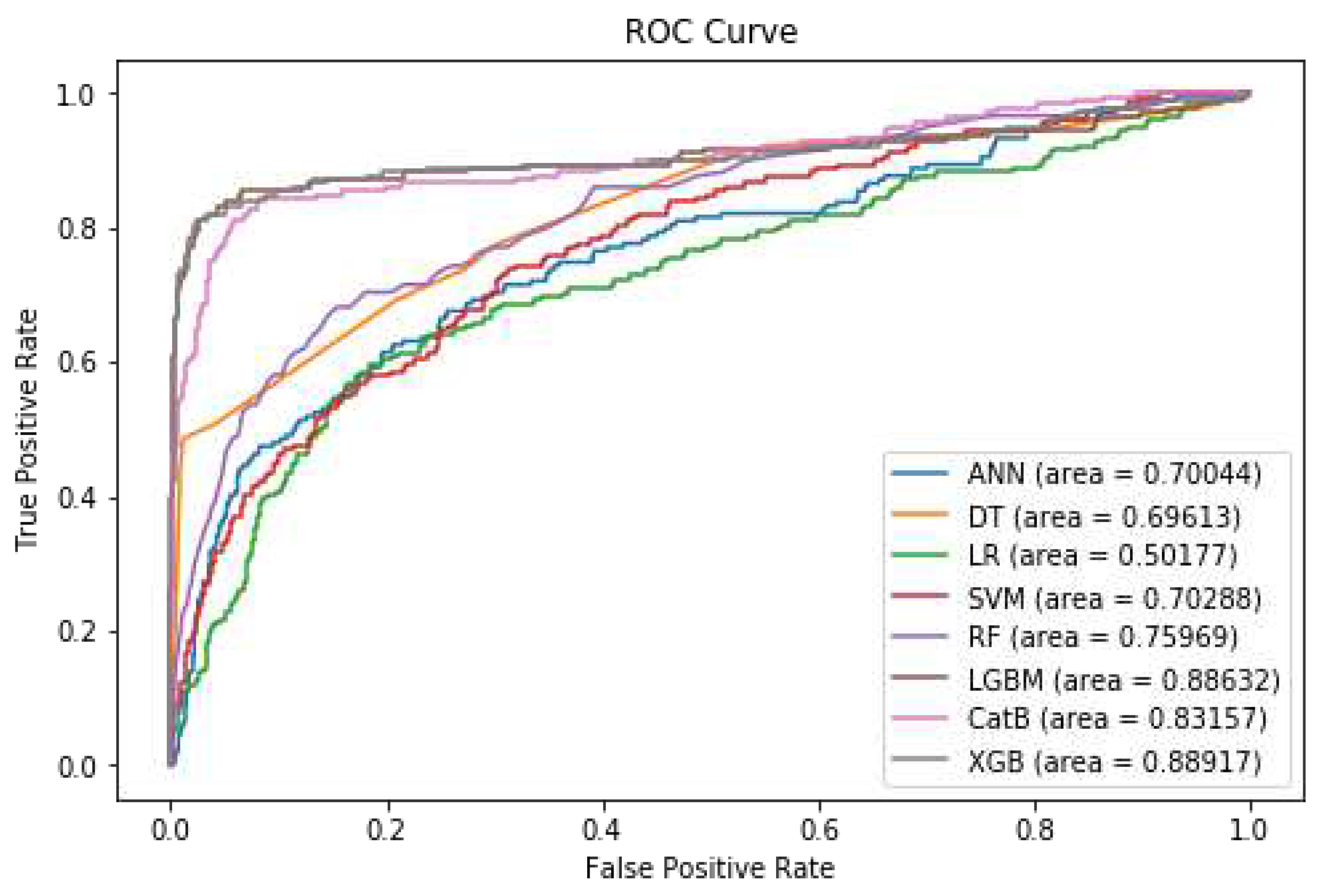
Table 6 shows, LightGBM and XGBoost outperform other ML techniques in all evaluation metrics. Notably, LightGBM and XGBoost surpass the performance of other methods, with both achieving an impressive ROC AUC of 90%, and XGBoost outperforms the other methods, achieving an impressive F1-Score of 92%.
Figure 8 shows the diagram of the ROC Curve for the different models after applying SMOTE.
6.2.3. Applying SMOTE with Tomek Links
As previously discussed in Section IV, the Tomek Links method is an undersampling technique that is used to identify pairs of examples, where each example belongs to a different class that has the minimum Euclidean distance to each other. Additionally, as noted in the section, it is beneficial to utilize a combination of both oversampling and undersampling techniques to achieve optimal results. The results of the evaluation metrics for the various models after applying the SMOTE technique in conjunction with Tomek Links are presented in
Table 7. Notably, LightGBM outperforms the other methods, achieving an impressive ROC AUC of 91%, and XGBoost surpasses the other methods, achieving an impressive F1-Score of 91%. As indicated in
Table 7, XGBoost demonstrates a marginal performance improvement, with a modest 2% enhancement in ROC AUC compared to the pre-processing and feature selection stage (initial state), as shown in
Table 6.
Figure 9 shows the diagram of the ROC Curve for the different models after applying SMOTE with Tomek Links.
6.2.4. Applying SMOTE with ENN
As previously discussed in Section IV, the ENN method is employed to compute the three nearest neighbors for each instance within the dataset. In instances where the sample belongs to the majority class and is misclassified by its three nearest neighbors, the instance is removed from the dataset. Conversely, if the instance belongs to the minority class and is misclassified by its three nearest neighbors, the three majority class instances are removed. Furthermore, as previously stated, it has been shown to be beneficial to utilize a combination of undersampling and oversampling techniques in order to achieve optimal results.
Table 8 illustrates the evaluation metrics for the various models following the application of the SMOTE technique in conjunction with the ENN method. The results indicate that XGBoost outperforms the other machine learning techniques, achieving an F1-Score of 88% and an ROC AUC of 89%. As indicated in
Table 8, XGBoost exhibits a performance decline, experiencing a 3% reduction in F1-Score compared to the pre-processing and feature selection stage (initial state), as shown in
Table 6.
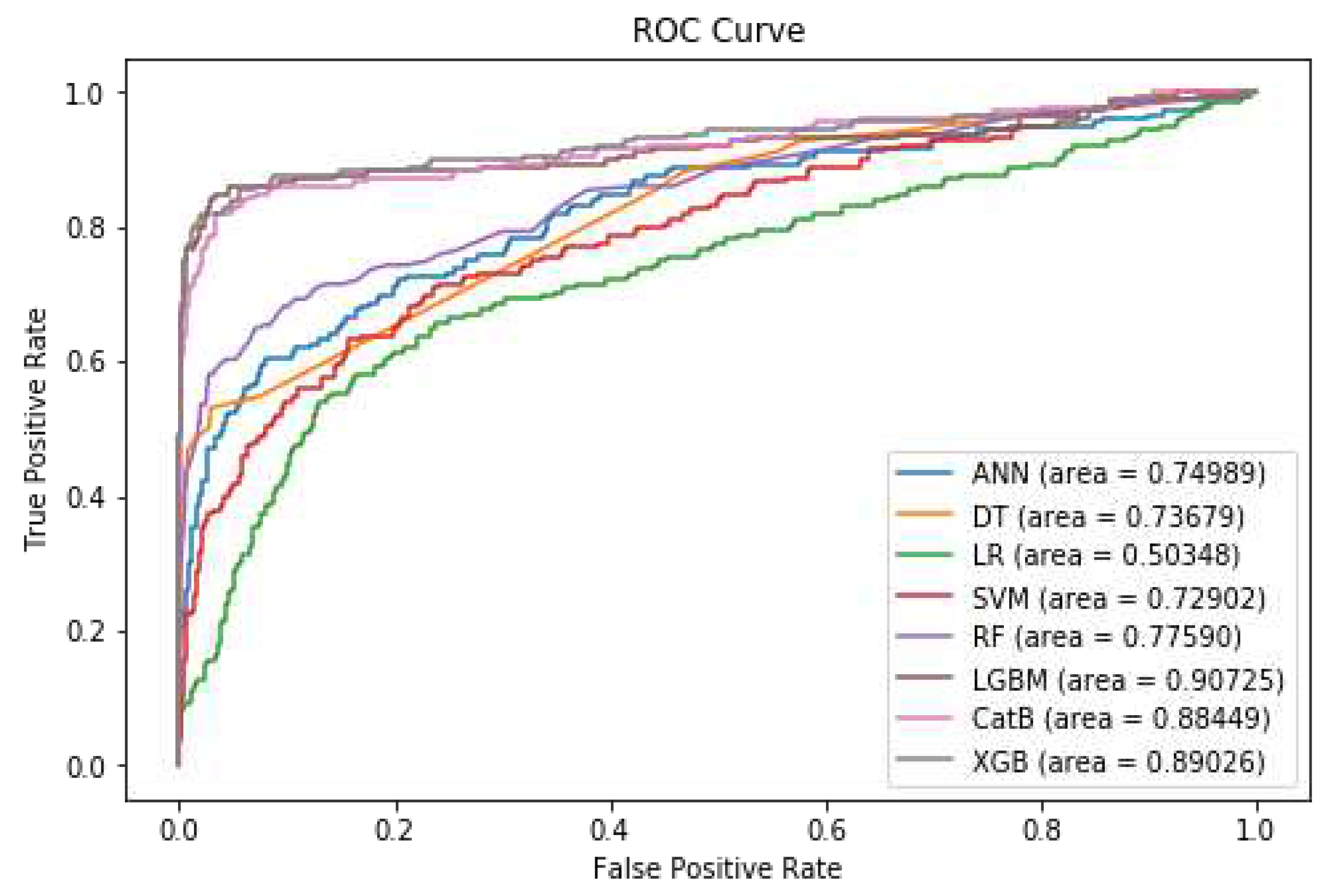
Figure 10 shows the diagram of the ROC Curve for the different models after applying SMOTE with ENN.
6.2.5. The Impact of Sampling Techniques
6.2.5.1. F1-Score:
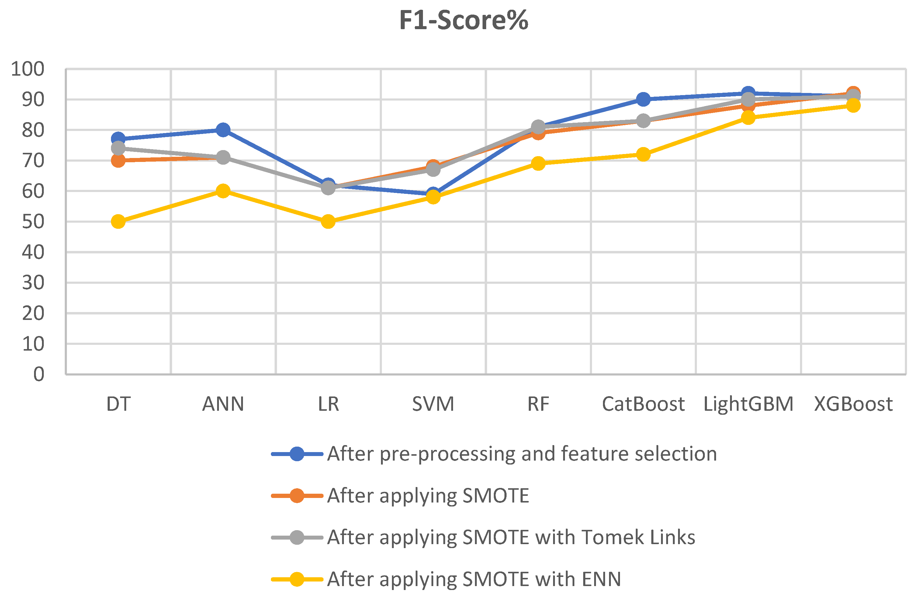
Table 9 and
Figure 11 show the impact of three distinct sampling techniques (SMOTE, SMOTE with Tomek Links, and SMOTE with ENN) on the F1-score metric of various machine learning models. These comparisons offer insights into the effectiveness of each technique in handling imbalanced datasets.
-
Impact of SMOTE Sampling Technique:
Most models saw a decrease in F1-Score after applying SMOTE compared to the pre-processing and feature selection stage (initial state).
CatBoost and LightGBM experienced a reduction in F1-Scores, but XGBoost showed slight improvements.
Support Vector Machine (SVM) exhibits enhanced F1-score.
-
Impact of SMOTE with Tomek Links Sampling Technique:
SMOTE with Tomek Links demonstrates further enhancements in F1-Scores for several models compared to SMOTE alone.
Support Vector Machine (SVM) showed improvements.
CatBoost experienced a reduction in F1-Scores compared to the pre-processing and feature selection stage (initial state).
LightGBM showed a slight reduction in F1-Scores by 2%.
XGBoost remained consistent with an F1-Score of 91.
-
Impact of SMOTE with ENN Sampling Technique:
SMOTE with ENN leads to varied impacts on F1-Scores across models.
Some models, like Decision Tree (DT), Logistic Regression (LR), and CatBoost experience significant drops in F1-Scores compared to the pre-processing and feature selection stage (initial state).
LightGBM maintain relatively high F1-Scores, with LightGBM achieving 84%.
XGBoost remains strong with an F1-score of 88% despite the decline.
SMOTE with ENN may not consistently enhance performance and should be chosen carefully based on the specific model and dataset characteristics.
In summary, the impact of different sampling techniques on F1-Scores varied across models. SMOTE generally led to reduced F1-Scores, with CatBoost and LightGBM experiencing declines and XGBoost showing slight improvements. SMOTE with Tomek Links enhanced F1-Scores for several models, particularly benefiting SVM, but CatBoost and LightGBM saw reductions. SMOTE with ENN had mixed effects on F1-Scores, significantly decreasing scores for some models but maintaining higher scores for LightGBM and XGBoost. Among the sampling techniques, SMOTE-ENN yields the least favorable results for all machine learning models when contrasted with methods such as SMOTE and SMOTE-TOMEK. Choosing the appropriate sampling technique should consider specific model and dataset characteristics.
6.2.5.2. ROC AUC:
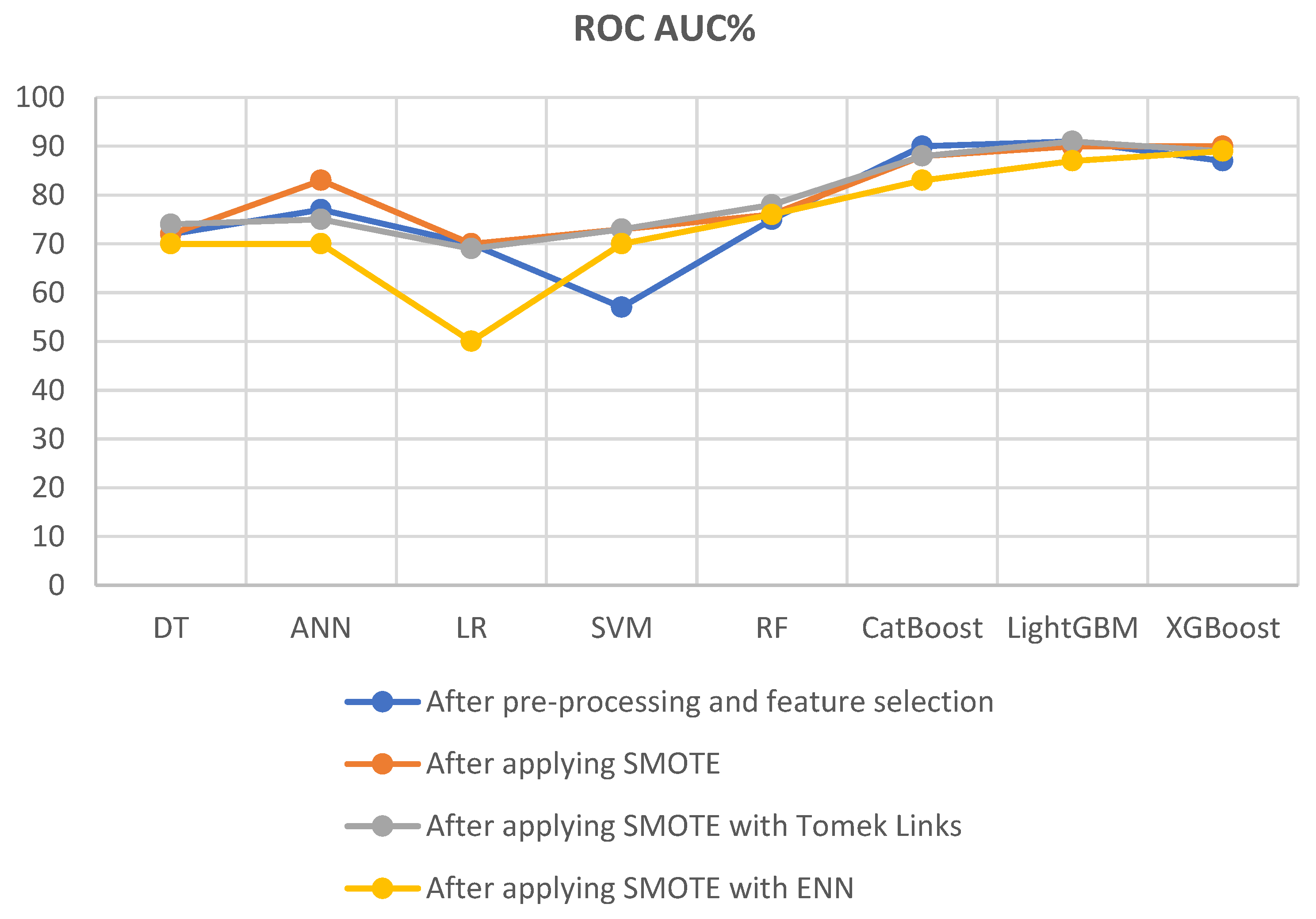
Table 10 and
Figure 12 show the impact of three distinct sampling techniques (SMOTE, SMOTE with Tomek Links, and SMOTE with ENN) on the ROC AUC metric of various machine learning models. These comparisons offer insights into the effectiveness of each technique in handling imbalanced datasets.
-
Impact of SMOTE Sampling Technique:
After applying SMOTE, there are noticeable improvements in ROC AUC metrics for some models.
ANN, SVM, RF, and XGBoost experience ROC AUC enhancements, but CatBoost, and LightGBM showed a slight reduction compared to the pre-processing and feature selection stage (initial state).
Models like ANN and SVM see substantial improvements, with ROC AUC scores reaching 83% and 73%, respectively.
-
Impact of SMOTE with Tomek Links Sampling Technique:
SMOTE combined with Tomek Links maintains or enhances ROC AUC metrics for most models.
DT, SVM, and RF observe improved ROC AUC metrics.
LightGBM and CatBoost maintain high ROC AUC scores of 91% and 88%, respectively.
This technique’s combination of class balancing (SMOTE) and removal of borderline instances (Tomek Links) continues to prove effective.
-
Impact of SMOTE with ENN Sampling Technique:
SMOTE with ENN produces mixed results for ROC AUC metrics.
While some models, like RF and XGBoost, and SVM showed improvements in ROC AUC metrics, others experienced drops.
Logistic Regression (LR) encounters a significant reduction in ROC AUC.
LightGBM maintains a respectable ROC AUC metric of 87%.
Researchers should exercise caution when applying SMOTE with ENN, as its impact varies across models.
In summary, the impact of different sampling techniques on ROC AUC metrics varied among models. SMOTE led to improvements for ANN, SVM, RF, and XGBoost but slight reductions for CatBoost and LightGBM. Notably, ANN and SVM achieved substantial ROC AUC scores of 83% and 73%, respectively. SMOTE with Tomek Links generally maintained or improved ROC AUC metrics, benefiting models like DT, SVM, RF, LightGBM, and CatBoost, with the latter two maintaining high scores. SMOTE with ENN produced mixed results, improving ROC AUC for some models, such as RF, XGBoost, and SVM, while causing a significant reduction in Logistic Regression. LightGBM maintained a respectable ROC AUC of 87%. Similar to the F1-score metric, SMOTE-ENN demonstrates lower performance in terms of ROC AUC for all machine learning models compared to techniques such as SMOTE and SMOTE-TOMEK. Researchers should select the most appropriate sampling technique based on their dataset and model to achieve optimal ROC AUC results.
6.2.5.3. Sampling Techniques vs Boosting Techniques:
Several factors contribute to the relatively modest impact of sampling techniques on the performance of boosting algorithms:
Iterative Nature: Boosting methods iteratively train a sequence of weak models, typically decision trees. Each subsequent model focuses on the errors made by the previous ones. Boosting is adaptive in the sense that it can adjust to the errors and potentially correct them in subsequent iterations.
Adaptive Nature: While oversampling introduces more instances of the minority class, boosting models, given their adaptive nature, can sometimes already compensate for the imbalance to some degree. As a result, oversampling might not always result in significant performance improvements.
Weighted Loss Function: Many boosting algorithms, like XGBoost, offer a weighted loss function where instances from different classes can be assigned different weights. This built-in mechanism can help in addressing class imbalance, reducing the need for external sampling methods.
In summary, while data sampling can rectify the decision boundary in models like SVM that are sensitive to class distributions, boosting techniques, due to their adaptive and iterative nature, might already have mechanisms to handle imbalance to a certain extent. However, the actual impact of sampling can vary based on the dataset, the degree of imbalance, the specific boosting algorithm used, and its hyperparameters.
6.2.6. Applying Optuna hyperparameter optimizer
Hyperparameter optimization is pivotal in machine learning for enhancing the performance of models. While models come with default hyperparameters, fine-tuning them to a specific dataset can substantially boost their efficacy. One prominent tool in this space is Optuna. Takuya Akiba et al. (2019) [
53] introduced Optuna, an open-source Python library for hyperparameter optimization. Optuna aims to balance the pruning and sampling algorithms through the execution of various techniques, such as the Tree-Structured Parzen Estimator (TPE) [
54,
55] for independent parameter sampling, Covariance Matrix Adaptation (CMA) [
56], and Gaussian Processes (GP) [
55] for relational parameter sampling. The library also utilizes a variant of the Asynchronous Successive Halving (ASHA) algorithm [
57] to prune search spaces.
TPE is a Bayesian optimization technique. Unlike grid or random search, which treats hyperparameters as isolated, TPE considers the relationship between hyperparameters and the objective function. The advantage of TPE over other methods lies in its efficiency. By constructing a probabilistic model of the objective function, it can suggest hyperparameters that are more likely to yield better results, hence reducing the number of trials [
54,
55].
Both CMA and GP are methodologies used in Optuna for relational parameter sampling. CMA captures the interdependencies between parameters, optimizing the sampling process, while GP uses the kernel trick to project data into higher dimensions, capturing complex relationships in the hyperparameter space [
55,
56].
The goal of ASHA is efficiency. It is an early stopping strategy to prune trials that do not show promise, which allows for a more efficient hyperparameter search. By identifying and halting unpromising trials early, computational resources are channeled more effectively [
57].
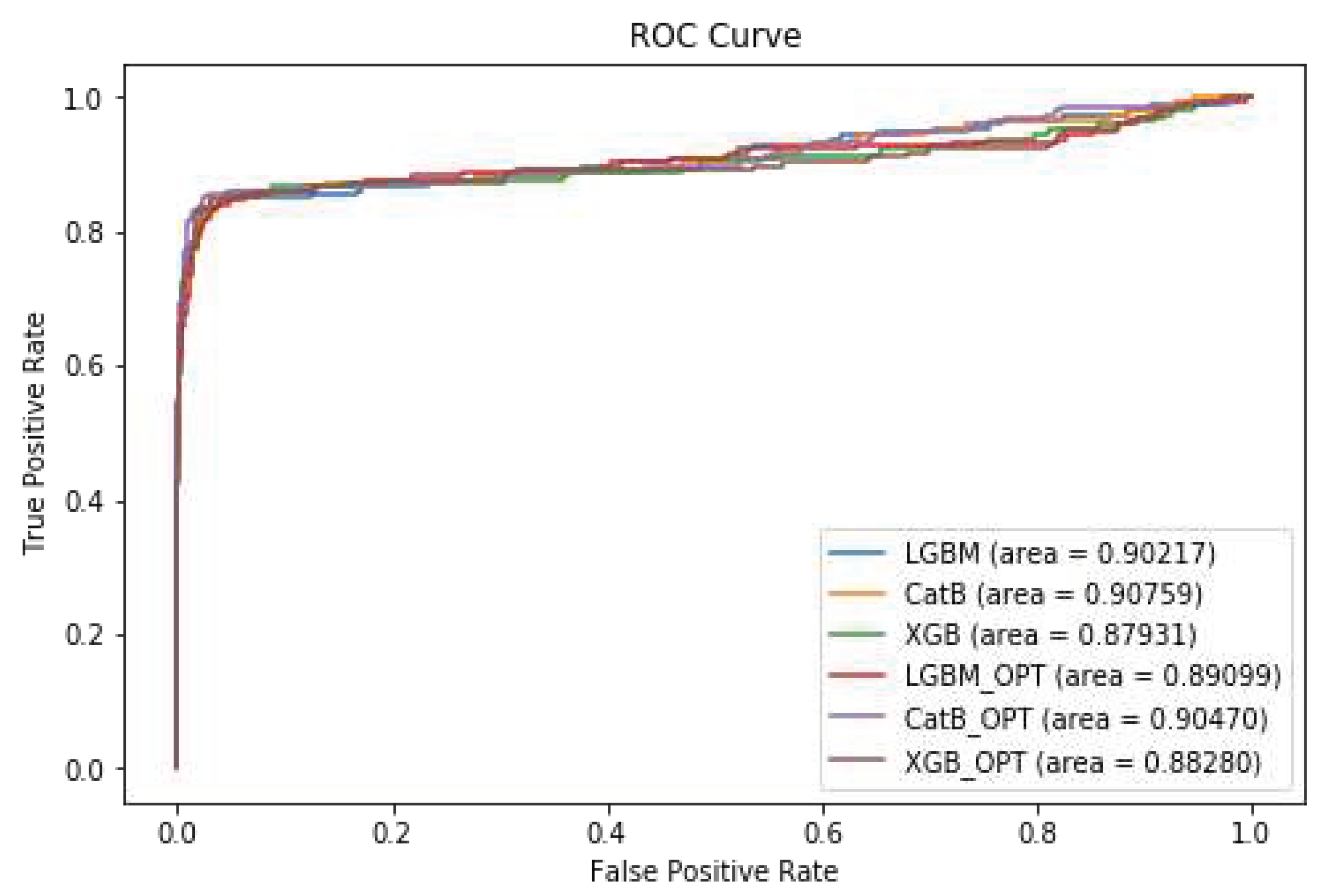
In this study, we applied the Optuna library to the popular machine learning models, CatBoost, XGBoost, and LightGBM. The results, as presented in
Table 11, indicate that CatBoost outperforms XGBoost and LightGBM when utilizing Optuna for hyperparameter optimization, achieving an impressive F1-Score of 93% and an ROC AUC of 91%. The improved F1-Score and ROC AUC results observed after employing Optuna hyperparameter tuning for CatBoost likely result from enhanced hyperparameter settings. Optuna fine-tunes these settings more effectively for your specific data, reducing overfitting and enhancing the models’ generalization to new data. This ultimately leads to improved overall model performance, as hyperparameters play a significant role in how effectively these algorithms operate with the dataset.
Figure 13 shows the diagram of the ROC Curve for the different models after applying Optunal hyperparameter tuning.
Table 12 includes all the parameters that were used in the XGBoost, LightGBM, and CatBoost models after applying Optuna hyperparameter tuning. The table provides a clear and concise summary of the parameter values that were selected for the models.
7. Conclusion
In this study, we employed various machine learning (ML) models, including Artificial Neural Networks, Decision Trees, Support Vector Machines, Random Forests, Logistic Regression, and three modern gradient boosting techniques, namely XGBoost, LightGBM, and CatBoost, to predict customer churn in the telecommunications industry using a real-world imbalanced dataset. We evaluated the impact of different sampling techniques, such as SMOTE, SMOTE with Tomek Links, and SMOTE with ENN, to handle the imbalanced data. We then assessed the performance of the ML models using various metrics, including Precision, Recall, F1-score, and Receiver Operating Characteristic Area Under the Curve (ROC AUC). Finally, we utilized the Optuna hyperparameter optimization technique on CatBoost, LightGBM, and XGBoost to determine the effect of optimization on the performance of the models. We compared the results of all the steps and presented them in tabular form.
The simulation results demonstrate the performance of different models on unseen data. LightGBM and XGBoost consistently exhibit superior performance across various evaluation metrics, including precision, recall, F1-Score, and ROC AUC. The performance of these models is further improved when applying techniques such as SMOTE with Tomek Links or SMOTE with ENN to handle imbalanced data. Additionally, the use of Optuna hyperparameter optimization for CatBoost, XGBoost, and LightGBM models shows further improvements in performance.
In summary, the key findings of the study are as follows:
- ❖
Impact of SMOTE: After applying SMOTE, both LightGBM and XGBoost achieved impressive ROC AUC scores of 90%. Additionally, XGBoost outperformed other methods with an impressive F1-Score of 92%. SMOTE effectively balanced class distribution, leading to enhanced recall and ROC AUC for most models.
- ❖
SMOTE with Tomek Links: After applying SMOTE with Tomek Links, LightGBM excelled among the methods with an impressive ROC AUC of 91%. XGBoost also outperformed other methods with an impressive F1-Score of 91%. LightGBM demonstrates a slight performance boost, with a modest 2% improvement in F1-Score and a 1% increase in ROC AUC compared to using SMOTE alone. Conversely, XGBoost showed a slight performance decline, experiencing a corresponding 1% reduction in F1-Score and ROC AUC compared to exclusive SMOTE utilization.
- ❖
SMOTE with ENN: After applying SMOTE with ENN, XGBoost surpassed other ML techniques, achieving an F1-Score of 88% and an ROC AUC of 89%. However, XGBoost exhibited a performance decline, with a 4% reduction in F1-Score and a 1% decrease in ROC AUC compared to exclusive SMOTE utilization.
The best results for F1-Score and ROC AUC across different ML models after applying various sampling techniques are summarized in
Table 13.
- ❖
Impact of Optuna Hyperparameter Tuning: After applying Optuna Hyperparameter Tuning, Cat-Boost outperformed XGBoost and LightGBM when Optuna was utilized for hyperparameter optimization, achieving an impressive F1-Score of 93% and an ROC AUC of 91%. The enhanced F1-Score and ROC AUC results observed after applying Optuna hyperparameter tuning to CatBoost, XGBoost, and LightGBM are likely attributable to improved hyperparameter configurations. Optuna fine-tuned these settings more effectively for the specific dataset, reducing overfitting and enhancing the models’ capacity to generalize to new data. This ultimately resulted in improved overall model performance, as hyperparameters significantly influence the performance of these algorithms with your dataset.
In future work, several avenues can be explored. Firstly, other machine learning techniques, such as deep learning models like Long Short-Term Memory (LSTM) or Transformer-based models, can be evaluated for churn prediction. These models have shown promise in various domains and may provide further insights into churn behavior. Secondly, we suggest exploring the use of the AdaSyn technique to handle imbalanced data and compare the results. Lastly, we recommend applying the above techniques to a highly imbalanced dataset to evaluate their performance in such conditions. Furthermore, employing the learning curve method to determine whether the models are overfitting could also be a valuable avenue of research.
Author Contributions
Writing and original draft preparation, subsequent revisions, coding, analysis, and interpretation of the results M.I.; supervision, review, and editing, H.R.A. All authors have read and agreed to the published version of the manuscript.
Funding
This research received no external funding.
Institutional Review Board Statement
Not applicable.
Informed Consent Statement
Not applicable.
Data Availability Statement
This study makes use of a publicly accessible dataset sourced from Kaggle [
58].
Conflicts of Interest
The authors declare no conflict of interest.
References
- The Chartered Institute of Marketing, “Cost of Customer Acquisition versus Customer Retention”, 2010.
- F. Eichinger, D.D. Nauck, F. Klawonn, “Sequence mining for customer behaviour predictions in telecommunications”, in: Proceedings of the Workshop on Practical Data Mining at ECML/PKDD, 2006, pp. 3–10.
- U.D. Prasad, S. Madhavi, “Prediction of churn behaviour of bank customers using data mining tools”, Indian J. Market. 42 (9) (2011) 25–30.
- Keramati, Abbas, Hajar Ghaneei, and Seyed Mohammad Mirmohammadi. “Developing a prediction model for customer churn from electronic banking services using data mining.” Financial Innovation 2.1 (2016): 1-13. [CrossRef]
- Scriney, Michael, Dongyun Nie, and Mark Roantree. “Predicting customer churn for insurance data.” International Conference on Big Data Analytics and Knowledge Discovery. Springer, Cham, 2020.
- De Caigny, Arno, Kristof Coussement, and Koen W. De Bock. “A new hybrid classification algorithm for customer churn prediction based on logistic regression and decision trees.” European Journal of Operational Research 269.2 (2018): 760-772. [CrossRef]
- K. Kim, C.-H. Jun, J. Lee, “Improved churn prediction in telecommunication industry by analyzing a large network”, Expert Syst. Appl. 41 (15) (2014) 6575–6584. [CrossRef]
- Ahmad, Abdelrahim Kasem, Assef Jafar, and Kadan Aljoumaa. “Customer churn prediction in telecom using machine learning in big data platform.” Journal of Big Data 6.1 (2019): 1-24. [CrossRef]
- De Caigny, Arno, Kristof Coussement, and Koen W. De Bock. “A new hybrid classification algorithm for customer churn prediction based on logistic regression and decision trees.” European Journal of Operational Research 269.2 (2018): 760-772. [CrossRef]
- R.J. Jadhav, U.T. Pawar, “Churn prediction in telecommunication using data mining technology”, IJACSA Edit. 2 (2) (2011) 17–19.
- D. Radosavljevik, P. van der Putten, K.K. Larsen, “The impact of experimental setup in prepaid churn prediction for mobile telecommunications: what to predict, for whom and does the customer experience matter?”, Trans MLDM 3 (2) (2010) 80–99.
- Y. Richter, E. Yom-Tov, N. Slonim, “Predicting customer churn in mobile networks through analysis of social groups”, SDM, vol. 2010, SIAM, 2010, pp. 732–741. [CrossRef]
- Amin, Adnan, et al. “Cross-company customer churn prediction in telecommunication: A comparison of data transformation methods.” International Journal of Information Management 46 (2019): 304-319. [CrossRef]
- K. Tsiptsis, A. Chorianopoulos, “Data Mining Techniques in CRM: Inside Customer Segmentation”, John Wiley & Sons, 2011.
- Joudaki, Majid, et al. “Presenting a New Approach for Predicting and Preventing Active/Deliberate Customer Churn in Telecommunication Industry.” Proceedings of the International Conference on Security and Management (SAM). The Steering Committee of the World Congress in Computer Science, Computer Engineering and Applied Computing (WorldComp), 2011.
- Amin, Adnan, et al. “Customer churn prediction in telecommunication industry using data certainty.” Journal of Business Research 94 (2019): 290-301. [CrossRef]
- E. Shaaban, Y. Helmy, A. Khedr, M. Nasr, “A proposed churn prediction model”, J. Eng. Res. Appl. 2 (4) (2012) 693–697.
- Khan, Yasser, et al. “Customers churn prediction using artificial neural networks (ANN) in telecom industry.” Editorial Preface From the Desk of Managing Editor 10.9 (2019). [CrossRef]
- Ho, Tin Kam. “Random decision forests.” Proceedings of 3rd international conference on document analysis and recognition. Vol. 1. IEEE, 1995.
- Breiman, Leo. “Random forests.” Machine learning 45.1 (2001): 5-32. [CrossRef]
- A. Amin, S. Shehzad, C. Khan, I. Ali, S. Anwar, “Churn prediction in telecommunication industry using rough set approach, in: New Trends in Computational Collective Intelligence”, Springer, 2015, pp. 83–95.
- I. H. Witten, E. Frank, M. A. Hall and C. J. Pal, Data Mining : Practical Machine Learning Tools and Techniques, San Francisco: Elsevier Science & Technology, 2016.
- A. Kumar and M. Jain, Ensemble Learning for AI Developers: Learn Bagging, Stacking, and Boosting Methods with Use Cases, Apress, 2020.
- M. Van Wezel and R. Potharst, “Improved customer choice predictions using ensemble methods,” European Journal of Operational Research, vol. 181, no. 1, pp. 436-452, 2007. [CrossRef]
- I. Ullah, B. Raza, A. K. Malik, M. Imran, S. U. Islam and S. W. Kim, “A churn prediction model using random forest: analysis of machine learning techniques for churn prediction and factor identification in telecom sector,” IEEE Access, pp. 60134-60149, 2019. [CrossRef]
- P. Lalwani, M. M. Kumar, J. Singh Chadha and P. Sethi, “Customer churn prediction system: a machine learning approach,” Computing, pp. 1-24, 2021. [CrossRef]
- Tarekegn, Adane, et al. “Predictive modeling for frailty conditions in elderly people: machine learning approaches.” JMIR medical informatics 8.6 (2020): e16678. [CrossRef]
- Ahmed, Mahreen, et al. “Exploring nested ensemble learners using overproduction and choose approach for churn prediction in telecom industry.” Neural Computing and Applications 32.8 (2020): 3237-3251. [CrossRef]
- B.E. Boser, I.M. Guyon, V.N. Vapnik, “A training algorithm for optimal margin classifiers”, in Proceedings of the Fifth Annual Workshop on Computational Learning Theory”, ACM, 1992, pp. 144–152.
- Y. Hur, S. Lim, “Customer churning prediction using support vector machines in online auto insurance service, in: Advances in Neural Networks” – ISNN 2005, Springer, 2005, pp. 928–933.
- S.J. Lee, K. Siau, A review of data mining techniques, Ind. Manage. Data Syst. 101 (1) (2001) 41–46. [CrossRef]
- Mazhari, N.,Imani, M., Joudaki, M. and Ghelichpour, A.,”An overview of classification and its algorithms” 3rd Data Mining Conference (IDMC’09): Tehran, 2009.
- G.S. Linoff, M.J. Berry, “Data Mining Techniques: For Marketing, Sales, and Customer Relationship Management”, John Wiley & Sons, 2011.
- Z.-H. Zhou, Ensemble Methods - Foundations and Algorithms, Taylor & Francis group, LLC, 2012.
- A. Kumar and M. Jain, Ensemble Learning for AI Developers: Learn Bagging, Stacking, and Boosting Methods with Use Cases, Apress, 2020.
- I. H. Witten, E. Frank, M. A. Hall and C. J. Pal, Data Mining : Practical Machine Learning Tools and Techniques, San Francisco: Elsevier Science & Technology, 2016.
- J. Karlberg and M. Axen, “Binary Classification for Predicting Customer Churn,” Umeå University, Umeå, 2020.
- D. Windridge and R. Nagarajan, “Quantum Bootstrap Aggregation,” in International Symposium on Quantum Interaction, 2017.
- J. C. Wang, T. Hastie, “Boosted varying-coefficient regression models for product demand prediction,” Journal of Computational and Graphical Statistics, vol. 23, no. 2, pp 361–382, 2014. [CrossRef]
- E Al Daoud, “Intrusion Detection Using a New Particle Swarm Method and Support Vector Machines,” World Academy of Science, Engineering and Technology, vol. 77, 59-62, 2013.
- E. Al Daoud, H Turabieh, “New empirical nonparametric kernels for support vector machine classification,” Applied Soft Computing, vol. 13, no. 4, 1759-1765, 2013. [CrossRef]
- E. Al Daoud, “An Efficient Algorithm for Finding a Fuzzy Rough Set Reduct Using an Improved Harmony Search,” I.J. Modern Education and Computer Science, vol. 7, no. 2, pp16-23, 2015. [CrossRef]
- Y. Zhang, A. Haghani. “A gradient boosting method to improve travel time prediction. Transportation Research Part C,” Emerging Technologies, vol. 58,308–324,2015. [CrossRef]
- A. Dorogush, V. Ershov, A. Gulin “CatBoost: gradient boosting with categorical features support,” NIPS, p1-7, 2017. M. Qi, K. Guolin, W. Taifeng, C. Wei, Y. Qiwei, M. Weidong, L. TieYan, “A Communication-Efficient Parallel Algorithm for Decision Tree,” Advances in Neural Information Processing Systems, vol. 29, pp. 1279-1287, 2016.
- M. Qi, K. Guolin, W. Taifeng, C. Wei, Y. Qiwei, M. Weidong, L. TieYan, “A Communication-Efficient Parallel Algorithm for Decision Tree,” Advances in Neural Information Processing Systems, vol. 29, pp. 1279-1287, 2016.
- A. Klein, S. Falkner, S. Bartels, P. Hennig, F. Hutter, “Fast Bayesian optimization of machine learning hyperparameters on large datasets,” In Proceedings of Machine Learning Research PMLR, vol. 54, pp 528-536,2017.
- Kubat, Miroslav, and Stan Matwin. “Addressing the curse of imbalanced training sets: one-sided selection.” Icml. Vol. 97. No. 1. 1997.
- Chawla, Nitesh V., et al. “SMOTE: synthetic minority over-sampling technique.” Journal of artificial intelligence research 16 (2002): 321-357. [CrossRef]
- Tomek, Ivan. “Two modifications of CNN.” (1976). [CrossRef]
- Wilson, Dennis L. “Asymptotic properties of nearest neighbor rules using edited data.” IEEE Transactions on Systems, Man, and Cybernetics 3 (1972): 408-421. [CrossRef]
- S. Tyagi and S. Mittal, “Sampling Approaches for Imbalanced Data Classification Problem in Machine Learning,” in Proceedings of ICRIC 2019, 2020.
- T. Fawcett, “An introduction to roc analysis”, Pattern Recogn. Lett. 27 (8) (2006) 861–874. [CrossRef]
- Akiba, Takuya, et al. “Optuna: A next-generation hyperparameter optimization framework.” Proceedings of the 25th ACM SIGKDD international conference on knowledge discovery & data mining. 2019.
- Bergstra, James, Daniel Yamins, and David Cox. “Making a science of model search: Hyperparameter optimization in hundreds of dimensions for vision architectures.” Proceedings of The 30th International Conference on Machine Learning. 2013.
- Bergstra, James S., et al. “Algorithms for hyper-parameter optimization.” Advances in Neural Information Processing Systems. 2011.
- Hansen, Nikolaus, and Andreas Ostermeier. “Completely derandomized self-adaptation in evolution strategies.” Evolutionary computation 9.2 (2001): 159-195. [CrossRef]
- Li, Liam, et al. “A system for massively parallel hyperparameter tuning.” Proceedings of Machine Learning and Systems 2 (2020): 230-246.
- Christy, R. (2020). Customer Churn Prediction 2020, Version 1. Retrieved January 20, 2022 from https://www.kaggle.com/code/rinichristy/customer-churn-prediction-2020.
Figure 1.
Visualization of the bagging approach.
Figure 1.
Visualization of the bagging approach.
Figure 2.
Visualization of the Random Forest classifier.
Figure 2.
Visualization of the Random Forest classifier.
Figure 3.
Visualization of the boosting approach.
Figure 3.
Visualization of the boosting approach.
Figure 4.
Comparison of tree growth methods. (a) XGBoost Level-wise tree growth. (b) LightGBM Leaf-wise tree growth.
Figure 4.
Comparison of tree growth methods. (a) XGBoost Level-wise tree growth. (b) LightGBM Leaf-wise tree growth.
Figure 6.
The Precision-Recall curve.
Figure 6.
The Precision-Recall curve.
Figure 7.
ROC Curve after pre-processing and feature selection.
Figure 7.
ROC Curve after pre-processing and feature selection.
Figure 8.
ROC Curve after applying SMOTE.
Figure 8.
ROC Curve after applying SMOTE.
Figure 9.
ROC Curve after applying SMOTE with Tomek Links.
Figure 9.
ROC Curve after applying SMOTE with Tomek Links.
Figure 10.
ROC Curve after applying SMOTE with ENN.
Figure 10.
ROC Curve after applying SMOTE with ENN.
Figure 11.
The Impact of Sampling Techniques on F1-score of Different ML Models.
Figure 11.
The Impact of Sampling Techniques on F1-score of Different ML Models.
Figure 12.
The Impact of Sampling Techniques on ROC AUC of Different ML Models.
Figure 12.
The Impact of Sampling Techniques on ROC AUC of Different ML Models.
Figure 13.
ROC Curve after Optuna hyperparameter tuning.
Figure 13.
ROC Curve after Optuna hyperparameter tuning.
Table 1.
Summary of important Acronyms.
Table 1.
Summary of important Acronyms.
| Acronym |
Meaning |
| ANN |
Artificial Neural Network |
| AUC |
Area Under Curve |
| BPN |
Back-Propagation Network |
| CatBoost |
Categorical Boosting |
| CNN |
Condensed Nearest Neighbor |
| DT |
Decision Tree |
| ENN |
Edited Nearest Neighbor |
| LightGBM |
Light Gradient Boosting Machine |
| LR |
Logistic Regression |
| ML |
Machine Learning |
| RF |
Random Forest |
| ROC |
Receiver Operating Characteristic |
| SMOTE |
Synthetic Minority Over-Sampling Technique |
| SVM |
Support Vector Machine |
| XGBoost |
eXtreme Gradient Boosting |
Table 2.
The confusion matrix for evaluating methods.
Table 2.
The confusion matrix for evaluating methods.
| |
Predicted class |
| Churners |
Non-churners |
| Actual class |
Churners |
TP |
FN |
| Non-churners |
FP |
TN |
Table 3.
ROC AUC benchmark for predicting churn.
Table 3.
ROC AUC benchmark for predicting churn.
| ROC AUC Threshold |
Description |
| ROC AUC< 50% |
Something is wrong * |
| 50%<= ROC AUC <60% |
Similar to flipping a coin |
| 60%<= ROC AUC <70% |
Weak prediction |
| 70%<= ROC AUC <80% |
Good Prediction |
| 80%<= ROC AUC <90% |
Very Good Prediction |
| ROC AUC >= 90% |
Excellent Prediction |
Table 4.
The names and types of different variables in the churn dataset.
Table 4.
The names and types of different variables in the churn dataset.
| Variable Name |
Type |
|
state, (the US state of customers) |
string |
|
account_length (number of active months) |
numerical |
|
area_code, (area code of customers) |
string |
|
international_plan, (whether customers have international plans) |
yes/no |
|
voice_mail_plan, (whether customers have voice mail plans) |
yes/no |
|
number_vmail_messages, (number of voice-mail messages) |
numerical |
|
total_day_minutes, (total minutes of day calls) |
numerical |
|
total_day_calls, (total number of day calls) |
numerical |
|
total_day_charge, (total charge of day calls) |
numerical |
|
total_eve_minutes, (total minutes of evening calls) |
numerical |
|
total_eve_calls, (total number of evening calls) |
numerical |
|
total_eve_charge, (total charge of evening calls) |
numerical |
|
total_night_minutes, (total minutes of night calls) |
numerical |
|
total_night_calls, (total number of night calls) |
numerical |
|
total_night_charge, (total charge of night calls) |
numerical |
|
total_intl_minutes, (total minutes of international calls) |
numerical |
|
total_intl_calls, (total number of international calls) |
numerical |
|
total_intl_charge, (total charge of international calls) |
numerical |
|
number_customer_service_calls, (number of calls to customer service) |
numerical |
|
churn, (customer churn – the target variable) |
yes/no |
Table 5.
Evaluation metrics for the different models after pre-processing and feature selection.
Table 5.
Evaluation metrics for the different models after pre-processing and feature selection.
| Models |
Precision% |
Recall% |
F1-Score% |
ROC AUC% |
| DT |
91 |
72 |
77 |
72 |
| ANN |
85 |
76 |
80 |
77 |
| LR |
61 |
70 |
62 |
70 |
| SVM |
81 |
57 |
59 |
57 |
| RF |
96 |
75 |
81 |
75 |
| CatBoost |
90 |
90 |
90 |
90 |
| LightGBM |
94 |
91 |
92* |
91* |
| XGBoost |
96 |
87 |
91 |
87 |
Table 6.
Evaluation metrics for the different models after applying SMOTE.
Table 6.
Evaluation metrics for the different models after applying SMOTE.
| Models |
Precision% |
Recall% |
F1-Score% |
ROC AUC% |
| DT |
69 |
72 |
70 |
72 |
| ANN |
70 |
73 |
71 |
83 |
| LR |
61 |
71 |
61 |
70 |
| SVM |
65 |
73 |
68 |
73 |
| RF |
83 |
76 |
79 |
76 |
| CatBoost |
79 |
88 |
83 |
88 |
| LightGBM |
87 |
90 |
88 |
90* |
| XGBoost |
95 |
90 |
92* |
90* |
Table 7.
Evaluation metrics for the different models after applying SMOTE with Tomek Links.
Table 7.
Evaluation metrics for the different models after applying SMOTE with Tomek Links.
| Models |
Precision% |
Recall% |
F1-Score% |
ROC AUC% |
| DT |
74 |
74 |
74 |
74 |
| ANN |
69 |
75 |
71 |
75 |
| LR |
61 |
70 |
61 |
69 |
| SVM |
65 |
73 |
67 |
73 |
| RF |
85 |
78 |
81 |
78 |
| CatBoost |
80 |
88 |
83 |
88 |
| LightGBM |
89 |
91 |
90 |
91* |
| XGBoost |
94 |
89 |
91* |
89 |
Table 8.
Evaluation metrics for the different models after applying SMOTE with ENN.
Table 8.
Evaluation metrics for the different models after applying SMOTE with ENN.
| Models |
Precision% |
Recall% |
F1-Score% |
ROC AUC% |
| DT |
60 |
70 |
50 |
70 |
| ANN |
61 |
70 |
60 |
70 |
| LR |
52 |
50 |
50 |
50 |
| SVM |
60 |
70 |
58 |
70 |
| RF |
67 |
76 |
69 |
76 |
| CatBoost |
70 |
83 |
72 |
83 |
| LightGBM |
80 |
89 |
84 |
87 |
| XGBoost |
88 |
89 |
88* |
89* |
Table 9.
F1-score of Different ML Models after Applying Different Sampling Techniques.
Table 9.
F1-score of Different ML Models after Applying Different Sampling Techniques.
| |
DT |
ANN |
LR |
SVM |
RF |
CatBoost |
XGBoost |
LightGBM |
| Initial |
77* |
80* |
62* |
59 |
81* |
90* |
92* |
91 |
| SMOTE |
70 |
71 |
61 |
68* |
79 |
83 |
88 |
92* |
| SMOTE-TOMEK |
74 |
71 |
61 |
67 |
81* |
83 |
90 |
91 |
| SMOTE-ENN |
50 |
60 |
50 |
58 |
69 |
72 |
84 |
88 |
Table 10.
ROC AUC of Different ML Models After Applying Different Sampling Techniques.
Table 10.
ROC AUC of Different ML Models After Applying Different Sampling Techniques.
| |
DT |
ANN |
LR |
SVM |
RF |
CatBoost |
XGBoost |
LightGBM |
| Initial |
72 |
77 |
70* |
57 |
75 |
90* |
91* |
87 |
| SMOTE |
72 |
83* |
70* |
73* |
76 |
88 |
90 |
90* |
| SMOTE-TOMEK |
74* |
75 |
69 |
73* |
78* |
88 |
91* |
89 |
| SMOTE-ENN |
70 |
70 |
50 |
70 |
76 |
83 |
87 |
89 |
Table 11.
Evaluation metrics for various models after applying Optuna hyperparameter optimization.
Table 11.
Evaluation metrics for various models after applying Optuna hyperparameter optimization.
| Models |
Precision% |
Recall% |
F1-Score% |
ROC AUC% |
| CatBoost |
89 |
91 |
90 |
91* |
| CatBoost-Optuna |
95 |
91 |
93* |
91* |
| LightGBM |
92 |
90 |
91 |
90 |
| LightGBM-Optuna |
93 |
89 |
90 |
89 |
| XGBoost |
93 |
88 |
90 |
88 |
| XGBoost-Optuna |
94 |
88 |
91 |
88 |
Table 12.
Optuna hyperparameter optimization parameters
Table 12.
Optuna hyperparameter optimization parameters
| Parameter |
Description |
Value |
| XGBoost Tuning Parameters |
| verbosity |
Verbosity of printing messages |
0 |
| objective |
Objective function |
binary:logistic |
| tree_method |
Tree construction method |
exact |
| booster |
Type of booster |
dart |
| lambda |
L2 regularization weight |
0.010281489790562261 |
| alpha |
L1 regularization weight |
0.0008440304772889829 |
| subsample |
Sampling ratio for training data |
0.8298281841818362 |
| colsample_bytree |
Sampling according to each tree |
0.9985902928710126 |
| max_depth |
Maximum depth of the tree |
7 |
| min_child_weight |
Minimum child weight |
2 |
| eta |
Learning rate |
0.12406825365082062 |
| gamma |
Minimum loss reduction required to make a further partition on a leaf node of the tree |
0.0004490383815764321 |
| grow_policy |
Controls a way new nodes are added to the tree |
depthwise |
| LightGBM Tuning Parameters |
| objective |
Objective function |
binary |
| metric |
Metric for binary classification |
binary_logloss |
| verbosity |
Verbosity of printing messages |
-1 |
| boosting_type |
Type of booster |
dart |
| num_leaves |
Maximum number of leaves in one tree |
1169 |
| max_depth |
Maximum depth of the tree |
10 |
| lambda_l1 |
L1 regularization weight |
2.689492421801289e-07 |
| lambda_l2 |
L2 regularization weight |
7.2387875465462e-08 |
| feature_fraction |
LightGBM will randomly select part of features on each iteration |
0.870805980078817 |
| bagging_fraction |
LightGBM will randomly select part of data without resampling |
0.6280893693081118 |
| bagging_freq |
Frequency for bagging |
7 |
| min_child_samples |
Minimum number of data in one leaf |
8 |
| CatBoost Tuning Parameters |
| Objective |
Objective function |
Logloss |
| colsample_bylevel |
Subsampling rate per level for each tree |
0.07760972009427407 |
| depth |
Depth of the tree |
12 |
| boosting_type |
Type of booster |
Ordered |
| bootstrap_type |
Sampling method for bagging |
Bayesian |
| bagging_temperature |
Controls the similarity of samples in each bag |
0.0 |
Table 13.
The best result of F1-Score and ROC AUC for different ML models.
Table 13.
The best result of F1-Score and ROC AUC for different ML models.
| Metrics/ Methods |
F1-Score |
ROC AUC |
| DT |
Initial = 77% |
SMOTE-TOMEK = 74% |
| ANN |
Initial = 80% |
SMOTE = 83% |
| LR |
Initial = 62% |
Initial and SMOTE = 70% |
| SVM |
SMOTE = 68% |
SMOTE and SMOTE-TOMEK = 73% |
| RF |
Initial and SMOTE-TOMEK = 81% |
SMOTE-TOMEK = 78% |
| CatBoost |
Initial = 90% |
Initial = 90% |
| XGBoost |
Initial = 92% |
Initial and SMOTE-TOMEK = 91% |
| LightGBM |
SMOTE = 92% |
SMOTE = 90% |
|
Disclaimer/Publisher’s Note: The statements, opinions and data contained in all publications are solely those of the individual author(s) and contributor(s) and not of MDPI and/or the editor(s). MDPI and/or the editor(s) disclaim responsibility for any injury to people or property resulting from any ideas, methods, instructions or products referred to in the content. |
© 2023 by the authors. Licensee MDPI, Basel, Switzerland. This article is an open access article distributed under the terms and conditions of the Creative Commons Attribution (CC BY) license (http://creativecommons.org/licenses/by/4.0/).
