On Some Features of the Magnetic Properties of Nuclear and Other Materials

Valeriy Kizka

doi:10.20944/preprints202308.1522.v1

Preprint

Short Note

On Some Features of the Magnetic Properties of Nuclear and Other Materials

This version is not peer-reviewed.

Valeriy Kizka^*

This version is not peer-reviewed.

Downloads

Views

Comments

Submitted:

22 August 2023

Posted:

22 August 2023

You are already at the latest version

Abstract

In this article, we have tried to extend the Neumann–Kopp law concerning the heat capacity of solid compounds to other physical observables for materials represented as mixtures of chemical compounds, alloys, and ceramics. The main goal of this study is to find the intervals of external or internal parameters for a solid compound, within which its physical observable - the magnetic transition temperature for this work, can be expressed in terms of the atomic or molar weighted sum of the magnetic transition temperatures of the constituent elements of a compound. Outside these intervals, we tried to figure out the structure of the variable by which the weighted sum should be multiplied. Thus, for USb–x(ThSb) mixtures with a mole fraction x from 0.36 to 0.55, the magnetic transition temperature of this mixture is expressed in term of the molar weighted sum of the temperature of uranium structural transition associated with a change in the magnetic properties of uranium and of the temperature at which the nature of the magnetic susceptibility of antimony changes. For the magnetic Laves phase compounds Er(Fe_0.8–xMn_0.2–yCo_x+y)₂, the Curie temperature of the compound is equal to the weighted sum of the Curie temperatures of all elements of the compound, except for Mn, at x = 0.1, y = 0 and y = 0.1. For the paramagnetic Curie temperature of intercalated dichalcogenides Cr_xМоSe₂, it can be expressed in terms of the weighted Neel temperature of chromium multiplied by a variable depending on x, on the atomic numbers of all elements of the compound, and on a parameter proportional to the derivatives with respect to x of the dichalcogenide’s crystal lattice parameters.

Keywords:

Neumann–Kopp law

;

magnetic properties

;

magnetism of actinides

;

Curie temperature

;

paramagnetic Curie temperature

Subject:

Physical Sciences - Condensed Matter Physics

According to the Neumann–Kopp law, the heat capacity of a solid compound A_wB_1–w is expressed as the sum of the weighted heat capacities of the compound elements: C = C_A⋅w + C_B⋅(1 – w), where w is the mass fraction of element A. This law is valid only in limited ranges of temperatures and values of w for each solid compound, for example [1]. It would be interesting to find out if it is possible to express any other physical observable for an arbitrary solid compound in the same way? It does not matter what kind of solid compound we take - a chemical compound, a mechanical mixture, an alloy or ceramics, first of all we want to consider the possibility of writing an arbitrary physical quantity in terms of an atomic or molar weighted sum of the physical quantities of the elements of the compound. In presiding work we considered mechanical properties of metal alloys under irradiation [2], and found that such description is possible in different intervals of radiation doses for different alloys. We also found that the thermophysical properties of various nuclear materials can also be expressed in terms of weighted sums of the thermophysical properties of the elements of materials [3,4,5]. In all of these results, weighted sums were multiplied by constants constructed from the atomic numbers of all the elements of a particular compound, chemical indices, or mass fraction values, and all of these constants did not equal one. Having a large set of such data for various materials, we can predict a new material with desired properties, which is currently done, in most cases, only thanks to the intuition of the experimenter. In this work, we continued to collect data, now on the magnetic characteristics of various materials.

Let us first consider the USb–x(ThSb) mixture, whose magnetic transition temperatures as a function of x are shown in Figure 1. All elements of this mixture are paramagnetic in all temperature ranges. Thorium is a temperature independent paramagnetic [6]. The mixture is either a ferromagnetic or an antiferromagnetic, depending on x. At first glance, it is impossible to apply the idea of representing the magnetic transition temperature of a mixture as a weighted sum of mole fractions of the magnetic transition temperatures of its elements. But we know that uranium exhibits a rapid increase in the crystallographic cell at T_U = 43 K [7], which coincides with a slight change in the magnetic susceptibility of U at approximately the same temperature [6]. Antimony has a magnetic susceptibility that does not depend on temperature down to T_Sb = 4 K, and below this temperature the magnetic susceptibility depends on temperature [8]. Thus, we can write the next formula for the temperature of magnetic transition of U_1-xTh_xSb:

T_{U_{1 - x} T h_{x} S b} (x) = [(1 - x) \cdot T_{U} + x \cdot T_{T h} + T_{S b}] \cdot q,

(1.1)

where q is some constant and T_Th = 0 K. Table 1 shows the experimental values of

T_{U_{1 - x} T h_{x} S b} (x)

and those calculated by (1.1) with adjusted q. Table 1 shows that at q = 5.34 and x ∈ [0.36, 0.55], formula (1.1) works very well with relative errors between the experimental and calculated temperatures of less than 1%.

Is the result obtained is accidental with a constant q in some range of x values? If we have such accidental coincidences for a large set of different materials and physical observables, then we can assume that this is a manifestation of some general physical law.

Let us consider magnetic the Laves phase compound Er(Fe_0.8–xMn_0.2–yCo_x+y)₂, which has ferromagnetic properties at certain x and y (Table 2) [9]. Manganese changes the Curie temperature of the compound, even though Mn is not a ferromagnetic. We will make calculation with and without Néel temperature T_N of Mn:

T_{C}^{E r {(F e_{0.8 - x} M n_{0.2 - y} C o_{x + y})}_{2}} = (T_{C}^{E r} + 2 \cdot (0.8 - x) \cdot T_{C}^{F e} + 2 \cdot (0.2 - y) \cdot T_{N}^{M n} + 2 \cdot (x + y) \cdot T_{C}^{C o}) \cdot q,

(1.2)

Where the Curie temperatures:

T_{C}^{E r}

= 18.74 K [10],

T_{C}^{F e}

= 1044 K [11],

T_{C}^{C o}

= 1390 K [12],

T_{N}^{M n}

= 100 K [13] or 0 K.

Table 2 shows that at q = 0.27 formula (1.2) describes the Curie temperatures of the compound Er(Fe_0.8–xMn_0.2–yCo_x_+y)₂ at x = 0.1, y = 0 and y = 0.1 with a relative error less than 1% without taking into account the magnetic temperature of Mn. The inclusion of the Néel temperature of Mn in the calculation worsens the relative error to 2.2%. It seems that we need to take T_C of all elements, while the characteristics of Mn are inside q. Is this result also a mere coincidence?

The fundamental question is, what is the nature of the variable q, which in some ranges of values of x becomes a constant? The electronic structure of a solid is determined by the atomic numbers (nuclear charges) of the elements of the solid, so you can write: q = q(atomic numbers). For different x, the lattice parameters of a crystalline solid change, which leads to a change in the physical observables that characterize the properties of the solid. So we can write: q = q(atomic numbers, x, lattice parameters). Considering the ceramics (Ni_1–xZn_x)Fe₂O₄ as an example, we now consider the structure of q.

This ceramics (Ni_1–xZn_x)Fe₂O₄ is a substitutional solid solution [14]. With a change in the content of Zn, which replaces Ni atoms, the Curie temperature of this ceramics changes (Table 3). The structure of the parameter q in (1.3′) is shown as follows:

T_{C}^{(N i_{1 - x} Z n_{x}) F e_{2} O_{4}} = ((1 - x) \cdot T_{C}^{N i} + 2 \cdot T_{C}^{F e}) \cdot q,

(1.3)

q = {(\frac{1}{(1 - x) \cdot N i} + \frac{1}{x \cdot Z n} + \frac{1}{2 \cdot F e} + \frac{h}{4 \cdot O})}^{- 1},

(1.3’)

where

T_{C}^{N i}

= 630 K [15],

T_{C}^{F e}

= 1044 K [11], atomic numbers: Ni = 28, Zn = 30, Fe = 26, O = 8. The form q is chosen in such a way as to fulfill the requirements of clarity and simplicity [2,3,4,5]. The variable h, which depends on the lattice parameters, is associated with the most electronegative element, although it can be placed anywhere within parentheses. Electronegativities: X(Ni) = 1.91 [16], X(Zn) = 1.65 [16], X(Fe) = 1.96 [16], X(O) = 3.44 [16]. Thus, we see that if there are elements in the compound that do not have a specific physical observable, in our case, the Curie temperature, then the presence of these elements is taken into account by their atomic numbers and by their mass or molar amounts in the compound. In Table 3, the Curie temperatures of ceramics, calculated by (1.3) with adjusted q, are presented in comparison with the experimental temperatures from [14]. For the resulting q, we calculated h (Table 3). It can be seen that for a fixed h for x = 0 and 0.2, the parameter q changes, although it is possible that both q and h are fixed in some ranges of external or internal parameters [2,3,4,5]. In this case, we multiply the weighted sum of the Curie temperatures by a variable depending on x and atomic numbers. Do we have a coincidence again?

In [3], we found that h is proportional to the first derivative with respect to x of the lattice parameters of the compound:

h = g \frac{\partial a}{\partial x},

where g is the gauge parameter, a is the lattice parameter of ceramics (cubic [14]). In table 3, we have only 3 points of x, so it is difficult to understand the properties of h, for this we consider the following complex compound.

The chromium-intercalated compound Cr_xMoSe₂ [17] has paramagnetic properties at room temperature, and at lower temperatures ( < 150 K) it has a magnetic ordering close to the ferromagnetic type, with always positive paramagnetic Curie temperatures Θ_p (Table 4). Of the three elements in Cr_xMoSe₂, only chromium has magnetic properties\transitions, but I did not find its paramagnetic Curie temperature, so I took its Néel temperature:

T_{N}^{C r}

= 311 K [18]. Probably, Θ_p of chromium is absent, since even at temperatures above

T_{N}^{C r}

the inverse magnetic susceptibility χ^–1 of Cr decreases, χ^–1 decreases from –195°C to temperatures above 1440°C [19]. Electonegativities: X(Cr) = 1.66 [16], X(Mo) = 2.16 [16], X(Se) = 2.55 [16] so we relate the parameter h to Se in (1.4′):

θ_{p}_{}^{C r_{x} M o S e_{2}} = x \cdot T_{N}^{C r} \cdot q,

(1.4)

q = {(\frac{1}{x \cdot C r} + \frac{1}{M o} + \frac{h}{2 \cdot S e})}^{- 1},

(1.4’)

where atomic numbers: Cr = 24, Mo = 42, Se = 34. The parameters q and h change for all x (Table 4). The change in the lattice parameters a and c depending on x for the hexagonal crystal structure of Cr_xMoSe₂ [17] is also shown in Table 4. The difference between the lattice parameters at the nearest x in Table 4 shows that h and a_i – a_i–1 and c_i – c_i–1 change synchronously according to the periodic law, so we approximated the lattice parameters by periodic functions (Figure 2).

Figure 2 shows that such a “good value” of χ²/ndf (should be around 1) is due to two reasons. First, we need to have more data points. Secondly, we need a good theory, from which the law of changing the lattice parameters with x follows organically, otherwise we fit the data to the function to which we want to fit the data. In any case, with such an approximation:

h = g_{1} \cdot \frac{\partial a}{\partial x} + g_{2} \cdot \frac{\partial c}{\partial x},

where g₁ and g₂ we still need to hack.

Thus, we have obtained that the magnetic properties of various materials can be represented by a molar-weighted sum of the magnetic properties of the elements of the materials. One has to conclude that either these are random coincidences that create the illusion of some kind of law, or these are manifestations of a real law, to clarify which a large database of physical properties of all elements of the periodic table, obtained with various values of internal and external parameters, is needed. With the help of this database, the prediction of a new complex compound with expected unique properties can be made not due to the intuition of the experimenter, as is currently done, but due to a clear knowledge of the relationships between the physical properties of the elements of a complex compound.

References

Valu et al. The low-temperature heat capacity of the (Th,Pu)O₂ solid solution. Journal of Physics and Chemistry of Solids 86 (2015) 194–206. [CrossRef]
V. Kizka. Relationship Between the Mechanical Properties of an Irradiated Metal Alloy and the Mechanical Properties of the Irradiated Elements of the Alloy. Preprints 2023 2023061366. [CrossRef]
[V. Kizka. Numerical Description of Melting/Solidification Temperature of Oxide Nuclear Fuels. Preprints 2023 2023050174. [CrossRef]
V. Kizka. Thermal Conductivity of Carbides and Nitrides of Zr, Th and U:Numerical Approach. Preprints 2023 2023030403. [CrossRef]
V. Kizka. Thermal Conductivity of ZrO2, ZrSiO4, (U,Zr)SiO4 and UO2: Numerical Approach. Preprints 2023 2023020406. [CrossRef]
K.G. Gurtovoĭ and R.Z. Levitin. Magnetism of actinides and their compounds. Sov. Phys. Usp. 30 (1987) 827. [CrossRef]
W. Suski. Magnetism of Uranium Intermetallics. Acta Physica Polonica A 91 (1997) 77. [CrossRef]
D. Shoenberg and M. Uddin. The magnetic properties of antimony. Mathematical Proceedings of the Cambridge Philosophical Society 32(3) (1936) 499–502. [CrossRef]
S. Othmani, I. Chaaba, S. Haj-Khlifa, P. de Rango, D. Fruchart. Magnetic and Magnetocaloric Effect of Laves Phase Compounds Er(Fe_0.8−xMn_0.2−yCo_x+y)₂ with x, y = 0.0 or 0.1. Metals 10 (2020) 1247. [CrossRef]
Rudy J.M. Konings and Ondrej Beneš. The Thermodynamic Properties of the f-Elements and Their Compounds. I. The Lanthanide and Actinide Metals. Journal of Physical and Chemical Reference Data 39(4) (2010) 043102–1 – 043102–47. [CrossRef]
J. Langner and J.R. Cahoon. Increase in the Alpha to Gamma Transformation Temperature of Pure Iron upon Very Rapid Heating. Metallurgical and Materials Transactions A 41(5) (2010) 1276–1283. [CrossRef]
E.B. Zaretsky. Impact Response of Cobalt over the 300-1400 K Temperature Range. Journal of Applied Physics 108(8) (2010) 083525–1 – 083525–7. [CrossRef]
A.C. Lawson, A.C. Larson, M.C. Aronson, S. Johnson, Z. Fisk, P.C. Canfield, J.D. Thompson, and R.B. Von Dreele. Magnetic and Crystallographic Order in α-Manganese. Journal of Applied Physics 76(10) (1994) 7049–7051. [CrossRef]
V.N. Shut, S.R. Syrtsov, L.S. Lobanovskii et al. Crystal structure and magnetic properties of (Ni_1–xZn_x)Fe₂O₄ composition graded ceramic. Phys. Solid State 58 (2016) 1975–1980. [CrossRef]
G. Schulze. Metallfhysik. Akademie-Verlag, Berlin 1967.
A. L. Allred. Electronegativity Values from Thermochemical Data. Journal of Inorganic and Nuclear Chemistry 17(3-4) (1961) 215–221.
V.G. Pleshchev, N.V. Selezneva. Magnetic Properties and Nature of Magnetic State of Intercalated CrxMoSe2 Compounds. Phys. Solid State 61 (2019) 339–344.
Eric Fawcett. Spin-density-wave antiferromagnetism in chromium. Rev. Mod. Phys. 60 (1988) 209.
T.R. McGuire and C.J. Kriessman. The Magnetic Susceptibility of Chromium. Phys. Rev. 85 (1952) 452.

Figure 1. Magnetic T-x phase diagram of the mixture USb–x(ThSb). The points were copied from [6].

Figure 2. The lattice parameters a and c of Cr_xMoSe₂ depending on x. The experimental points were taken from [17]. The curves are an approximation with respect to the functions depicted at the bases of the figures.

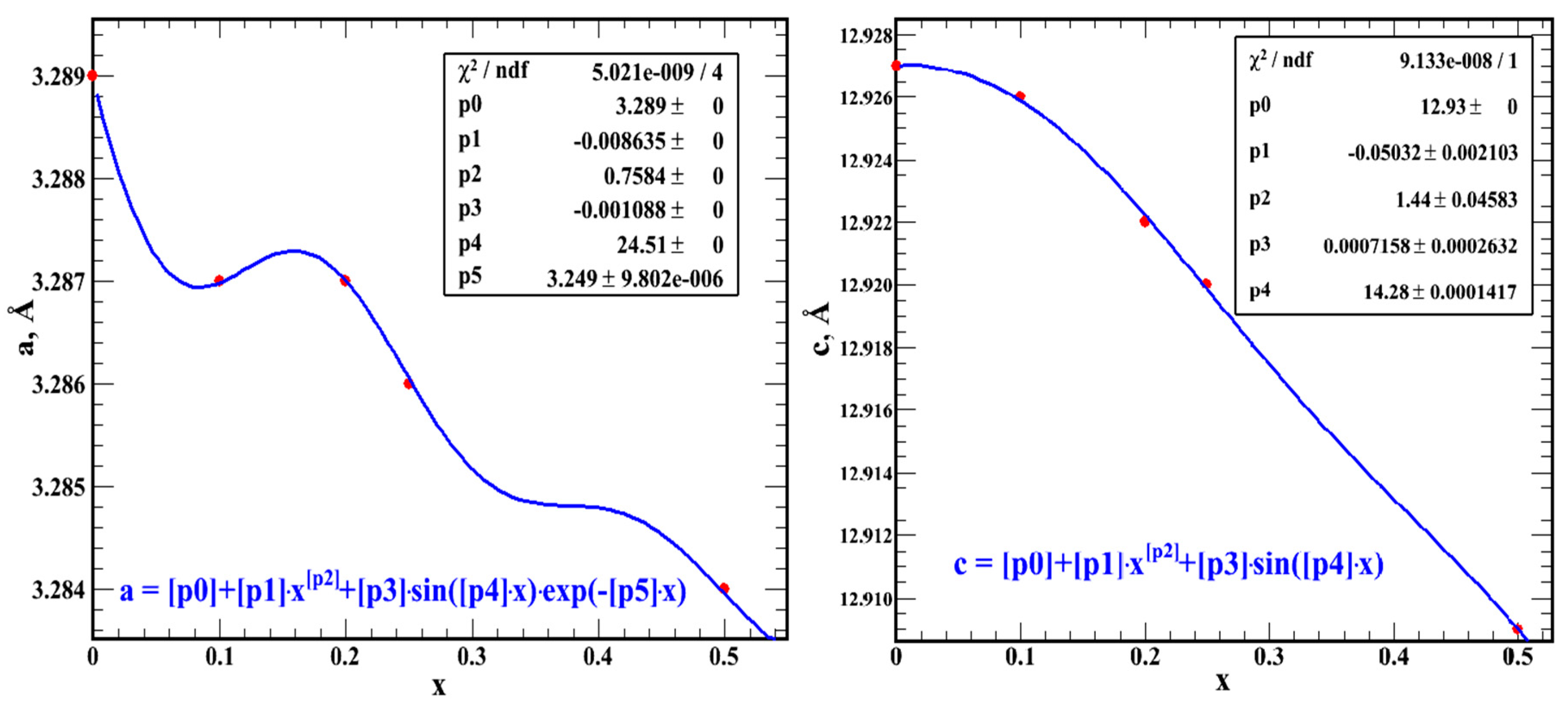
Table 1. Temperatures of magnetic transitions of U_1-xTh_xSb at various x taken from experiment [6]

T_{U_{1 - x} T h_{x} S b} {(x)}_{\exp}

and calculated by (1.1) (

T_{U_{1 - x} T h_{x} S b} {(x)}_{t h e o r y}

) with adjusted q. Relative errors δ were calculated by the following formula:

δ = | 1 - \frac{T_{U_{1 - x} T h_{x} S b} {(x)}_{t h e o r y}}{T_{U_{1 - x} T h_{x} S b} {(x)}_{\exp}} | \cdot 100 % .

Table 1. Temperatures of magnetic transitions of U_1-xTh_xSb at various x taken from experiment [6]

T_{U_{1 - x} T h_{x} S b} {(x)}_{\exp}

and calculated by (1.1) (

T_{U_{1 - x} T h_{x} S b} {(x)}_{t h e o r y}

) with adjusted q. Relative errors δ were calculated by the following formula:

δ = | 1 - \frac{T_{U_{1 - x} T h_{x} S b} {(x)}_{t h e o r y}}{T_{U_{1 - x} T h_{x} S b} {(x)}_{\exp}} | \cdot 100 % .

x	$T_{U_{1 - x} T h_{x} S b} {(x)}_{\exp}$ , K	$T_{U_{1 - x} T h_{x} S b} {(x)}_{t h e o r y}$ , K	q	δ,%
0.055	198.90	200.86	4.50	0.1
0.100	184.11	185.74	4.35	0.9
0.142	182.47	181.98	4.45	0.3
0.217	181.64	180.81	4.80	0.5
0.298	177.53	177.77	5.20	0.1
0.365	166.85	167.17	5.34	0.2
0.422	155.34	154.08	5.34	0.8
0.479	142.19	141.00	5.34	0.8
0.549	124.93	124.92	5.34	0.008
0.602	110.14	110.85	5.25	0.6
0.690	83.83	83.18	4.80	0.8
0.764	56.71	56.59	4.00	0.2
0.810	38.63	38.94	3.20	0.8
0.866	11.50	11.71	1.20	1.8

Table 2. The Curie temperatures T_{C exp} of Er(Fe_0.8–xMn_0.2–yCo_x+y)₂ were taken from the experiment [9] and calculated according to (1.2)(T_{C theory}) with adjusted q. Calculated T_C by (1.2) with

T_{N}^{M n}

= 100 K are shown separately ”with Mn in (1.2)” and the same for relative errors:

δ = | 1 - \frac{T_{C} {(x, y)}_{t h e o r y}}{T_{C} {(x, y)}_{\exp}} | \cdot 100 % .

T_{N}^{M n}

= 100 K are shown separately ”with Mn in (1.2)” and the same for relative errors:

δ = | 1 - \frac{T_{C} {(x, y)}_{t h e o r y}}{T_{C} {(x, y)}_{\exp}} | \cdot 100 % .

Compound	T_{C exp}, K	T_{C theory}, K	T_{C theory}, K with Mn in (1.2)	q	δ,%	δ,% with Mn in (1.2)
Er(Fe_0.8Mn_0.2)₂	355	354.7	354.5	0.21	0.08	2.6
Er(Fe_0.8Mn_0.1Co_0.1)₂	550	550.8	556.4	0.28	0.1	1.2
Er(Fe_0.7Mn_0.2Co_0.1)₂	475	474.5	485.5	0.27	0.1	2.2
Er(Fe_0.7Mn_0.1Co_0.2)₂	555	549.8	555.2	0.27	0.9	0.04

Table 3. The Curie temperatures T_{C exp} of (Ni_1–xZn_x)Fe₂O₄ were taken from the experiment [14] and calculated by (1.3) (T_{C theory}) with adjusted q and h by (1.3′). Relative errors δ were calculated by the next formula:

δ = | 1 - \frac{T_{C} {(x)}_{t h e o r y}}{T_{C} {(x)}_{\exp}} | \cdot 100 % .

δ = | 1 - \frac{T_{C} {(x)}_{t h e o r y}}{T_{C} {(x)}_{\exp}} | \cdot 100 % .

x	T_{C exp}, K	T_{C theory}, K	h	q	δ,%
0	790	792.4	108	0.291	0.3
0.1	740	741.7	102	0.279	0.2
0.2	720	718.9	108	0.277	0.2

Table 4. The paramagnetic Curie temperatures Θ_{p exp} of Cr_xMoSe₂ were taken from experiment [17] and calculated by (1.4) (Θ_{p theory}) with adjusted q and h by (1.4′). The lattice parameters were taken from [17]. Relative errors δ were calculated by the next formula:

δ = | 1 - \frac{θ_{p} {(x)}_{t h e o r y}}{θ_{p} {(x)}_{\exp}} | \cdot 100 % .

δ = | 1 - \frac{θ_{p} {(x)}_{t h e o r y}}{θ_{p} {(x)}_{\exp}} | \cdot 100 % .

x	Θ_{p exp}, K	Θ_{p theory}, K	q	h	a, Å	a_i – a_i–1, pm	c, Å	c_i – c_i–1, pm	δ,%
0					3.289		12.927
0.1	10	10.07	0.322	180	3.287	– 0.2	12.926	– 0.1	0.7
0.2	8	8.06	0.129	495	3.287	0	12.922	– 0.4	0.75
0.25	15	15.06	0.194	321	3.286	– 0.1	12.920	– 0.2	0.4
0.33	50	50.22	0.488	109					0.4
0.5	43	42.99	0.277	216	3.284	– 0.2	12.909	– 1.1	0.02

Disclaimer/Publisher’s Note: The statements, opinions and data contained in all publications are solely those of the individual author(s) and contributor(s) and not of MDPI and/or the editor(s). MDPI and/or the editor(s) disclaim responsibility for any injury to people or property resulting from any ideas, methods, instructions or products referred to in the content.

© 2023 by the authors. Licensee MDPI, Basel, Switzerland. This article is an open access article distributed under the terms and conditions of the Creative Commons Attribution (CC BY) license (http://creativecommons.org/licenses/by/4.0/).

Copyright: This open access article is published under a Creative Commons CC BY 4.0 license, which permit the free download, distribution, and reuse, provided that the author and preprint are cited in any reuse.

Downloads

Views

Comments

Subscription

Notify me about updates to this article or when a peer-reviewed version is published.

MDPI Initiatives

Important Links

Choose an area of interest and we will send you notifications of new preprints at your preferred frequency.

Disclaimer

On Some Features of the Magnetic Properties of Nuclear and Other Materials

Abstract

Keywords:

Subject:

References

MDPI Initiatives

Important Links

Subscribe