Preprint
Article

PEMFC Performance Forecasting Based on XGBRegressor and Tree-Structured Parzen

Altmetrics

Downloads

206

Views

146

Comments

0

Submitted:

21 August 2023

Posted:

22 August 2023

You are already at the latest version

Alerts
Abstract
The proton exchange membrane fuel cell (PEMFC) is a critical and essential component of zero-emission electro-hydrogen generators. An accurate prediction of its performance is important for optimal operation management and preventive maintenance of these generators. However, the prediction is not simple because the PEMFCs have complex electrochemical reactions with multiple nonlinear relations between operating variables as inputs and voltage as output. In this paper, we propose an efficient prediction approach based on XGBRegressor and Tree-structured Parzen Estimator. In addition, to better select relevant features, Kernel Principal Component Analysis and Mutual Information are jointly used. The proposed approach allows consideration of the dynamic operating conditions of the PEMFC. To test and validate the robustness of the proposed approach, a real data-set of ten PEMFCs was considered. Furthermore, a comparison study with traditional machine learning models, such as artificial neural networks and support vector machine regression, was investigated. The obtained results confirm that our model outperforms the considered traditionel machine learning models.
Keywords: 
Subject: Computer Science and Mathematics  -   Artificial Intelligence and Machine Learning

1. Introduction

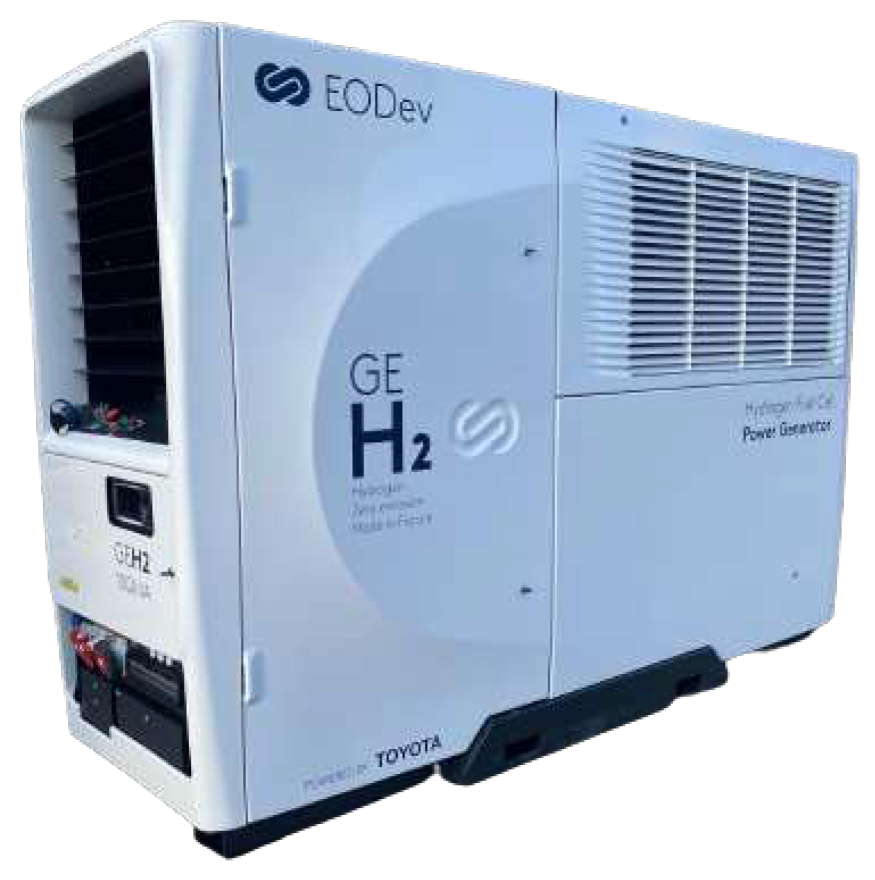
Renewable energies have become a fundamental part of the current energy mix. These energy sources are the most sustainable and eco-friendly, in contrast to fossil fuels, which release greenhouse gases and contribute to climate change. In this context, Energy Observer Development (EODev) aims to make their use more widespread, particularly that of hydrogen as an energy carrier for a low-carbon society. The GEH2 zero-emission electro-hydrogen generator (Figure 1) is the most compact and efficient electro-hydrogen generator on the market, in terms of power output. The GEH2 uses proton exchange membrane fuel cell (PEMFC) running on di-hydrogen to perform its functions. The latter requires auxiliary systems to operate, such as pumps, cooling systems and power supplies. To optimize the PEMFC’s service life and meet customer requirements, the GEH2 also incorporates a 47kWh battery. Power conversion and control systems ensure smooth operation. With the aim of reducing its environmental impact, durability, reliability and efficiency are key development priorities for the design and use of the GEH2. To ensure the smooth operation of GEH2 equipment, EODev is currently following a systematic maintenance plan comprising over 50 operations. EODev would therefore like to move towards a more predictive type of maintenance, so as to deploy actions only in relation to the actual state of a GEH2 unit. To provide answers to this industrial challenge, the goal of this work is to develop prognostic approaches for predicting the state of health of key components of the GEH2 electro-hydrogen unit. Since PEMFC is one of the critical comopsants of GEH2. In this paper, we present a machine learning-based approach for predicting the performance of PEMFC.
The PEMFC is a promising technology in fuel cells, offering a clean and efficient alternative to traditional energy sources. It is operated in conjunction with a battery (as the case of the zero-emission electro-hydrogen generator) or a supercapacitor module to meet the efficiency requirements. In fact, evaluating the performance of a PEMFC typically involves measuring a polarization curve which represents the relationship between the current density and the voltage of the fuel cell. This curve is significantly affected by various operating variables of the PEMFC, such as current, temperature, pressure, etc. According to [8,24], the polarization curve is selected as the focal point for the performance prediction model due to its ability to encompass crucial properties of PEMFC, including current density, voltage, and other significant factors. Currently, there are three main kinds of approaches employed to analyze the performance of PEMFC: model-driven approach, hybrid approach, and data-driven approach.
The model-driven approach forecasts the PEMFCs’ performance based on physical and mathematical models of the electrochemical, transport, and thermal processes that occur. These models can simulate PEMFC performance in a range of operational conditions and do not require a large amount of data to construct the model. They depend on a thorough understanding of the underlying operational mechanisms and interactions between components and incorporate temporal and spatial elements into their analyses. Kishimoto et al. [34] created a numerical methodology for predicting the electrochemical characteristics that takes into account various features, such as current-voltage behavior, macroscopic properties, and impedance. Talukdar et al. [34] explored the correlation between electrode performance and drying techniques. They achieved this by constructing a dynamic two-dimensional physical continuum model that incorporates the sensitivity of catalyst layer microstructure parameters. Danilov and Tade [36] have developed a new technique for estimating cathodic and anodic charge transfer coefficients from PEMFC voltage-current curves. In [37], an equation was formulated to fit the cell potential to current density data for PEMFCs in different conditions. This equation includes an exponential term to take into consideration the effects of mass transport, which allows for the capture of slope changes and a rapid potential drop. Guinea et al. [38] have developed another voltage-current model that takes into account the electron leakage current density, so that accurate matching performance can be achieved using gradient optimization methods and rotational.
The hybrid approach predicts the PEMFCs’ performance based on both physical models and historical data. For example, Bressel et al. [39] proposed a novel approach based on an Extended Kalman Filter-based observer to accurately estimate both the health status and degradation dynamics. Wang et al. [8] presented a new method that combines the benefits of machine learning methods and semi-empirical models to predict the degradation of a PEMFC system with 300 cells. Hu et al. [41] proposed a hybrid method for predicting the probability of performance degradation in PEMFCs, with the goal of extending service life and reducing maintenance costs. Pan et al. [42] introduced a hybrid methodology that combines a model-based adaptive Kalman filter with a data-driven NARX neural network to predict the degradation of PEMFCs. The overall degradation trend is captured through an empirical aging model and an adaptive Kalman filter, while the intricate degradation specifics are depicted using the NARX neural network. Zhou et al. [31] combined a physical aging model and time-delay neural networks to forecast the deterioration of a PEMFC. The physical aging model was used to remove the non-stationary trend from the original data, and the linear component was filtered with an autoregressive and moving-average model. The remaining non-linear model was then used to train the delayed neural networks, which were used to make the final prediction. Cheng et al. [43] proposed a method to enhance the precision of prognostic results when characterization is uncertain. They used the least square support vector machine (LSSVM) for initial prognostics and subsequently employed a regularized particle filter (RPF) to determine the final probability distribution of Remaining Useful Life (RUL) for PEMFC.
The application of the model-driven and hybrid approaches requires a certain level of physical knowledge about the system behavior, leading to some difficulties in some real and complex applications. In this context, the data-driven approach predicting the PEMFC purely based on historical data has been extensively developed thanks to their remarkable flexibility and their strong predictive capabilities. For example, Wilberforce et al. [28] employed an ANN to predict the current and voltage of PEMFC, minimizing the power required for fuel pumping and thus reducing net losses in the cell. Legala et al. [24] carried out a comparative study between ANN and SVR for predicting variables such as cell voltage, membrane resistance, etc. The study showed that ANN is better than SVR, particularly in multivariate output regression tasks. However, SVR shows its strength in simpler regressions, offering reduced computational load while maintaining accuracy. Han et al. [19] combined ANN and SVM to predict the PEMFC stack performance, considering the influence of different operating conditions of the PEMFC. In [20], they used a deep belief network (DBN) to build a model to predict the performance and maximize the power density of a PEMFC. Also, in [22] they used a long short-term memory (LSTM) to predict the performance of PEMFC under dynamic conditions, especially for vehicle applications. Chen et al. [10] applied a gradient backpropagation neural network to anticipate the aging evolution of PEMFCs. The parameters of this model were adjusted by an evolutionary algorithm, including a mental evolutionary algorithm (MEA), particle swarm optimization (PSO), and genetic algorithm (GA). Zou et al. [47] have advanced an RNN model with an attention mechanism to optimize prognostic and health management predictions, thus promoting more accurate anticipation of output voltage deterioration in PEMFC. He et al. [48] proposed an auto-encoder (AE)-LSTM network model to predict PEMFC degradation progress and mechanisms, during vehicle operation. This strategy employs a health indicator to represent PEMFC degradation states, followed by LSTM analysis.
Nevertheless, a significant limitation of the existing models is that they are not generic enough to be adapted to different PEMFC configurations, as in the case of GEH2 PEMFC. Also, most of the machine learning models used to predict PEMFC performance have not been evaluated on real data sets or they do not take into account the dynamic operating conditions of PEMFC. Additionally, some models, such as deep neural networks, can be considered black boxes in the sense that they provide predictions without offering a clear explanation of the underlying causal relationships. This can make it difficult to interpret the results and understand the factors influencing the polarization curve. In short, a new modeling approach is needed to provide a better prediction of PEMFC performance. Therefore, we propose in this paper an efficient prediction approach based on XGBRegressor and Tree-structured Parzen Estimator. In addition, Kernel Principal Component Analysis and Mutual Information are jointly used to better select relevant features. The proposed approach allows considering the dynamic operating conditions of the PEMFC. To test and validate the robustness of the proposed approach and also to cover different operating conditions, a real industrial data set of ten PEMFCs was used. Furthermore, a comparison study with other machine learning models, such as artificial neural networks and support vector machine regressions, is investigated. The main contributions of this study can be summarized as follows:
  • A new feature selection method based on KPCA and Mutual Information was developed to select the relevant features that control the PEMFC.
  • A novel performance prediction method based on XGBRegressor and Tree-structured Parzen Estimator was proposed to predict the polarization curve of the PEMFC.
  • A comparison study between the proposes model and traditional machine learning models has been carried out on a real dataset.
The rest of the paper is organized as follows: Section 2 describes the studied data and PEMFC feature selection. Section 3 presents the proposed prediction model based on XGBRegressor and Tree-structured Parzen Estimator. In Section 4, the performance of the proposed method is evaluated using actual polarization curve data of ten PEMFCs. Furthermore, a comparison study with two popular machine learning regressors widely used to predict the polarisation curve: artificial neural network (ANN) and support vector machine regressor (SVR) is also given. Finally, this work’s conclusions are discussed in Section 5.

2. Experimental Data and Dimensionality Reduction

In this section, we explain how the data was collected from different electro-hydrogen generators under different operating conditions. In addition, the feature selection of the PEMFC is given.

2.1. Data Description

The experimental data were provided by EODev, a company specializing in the manufacture of zero-emission electro-hydrogen generators. These generators are composed of different main components and the PEMFCs play a crucial and essential role in EODev’s generators, allowing them to produce the necessary energy or charge the battery under varying conditions. With over 100 generators deployed worldwide, PEMFCs can operate effectively in a variety of environments, allowing us to obtain different types of data that we use to validate our work. Each generator has sensors to measure various system parameters. These include polarization curve parameters such as current, tension, temperature, pressure, etc. The polarization curves were therefore obtained directly from the data collected by the various GeH2 sensors. More than 23 variables of PEMFCs are monitored in real time. Some of them could be controlled to more precisely manage the operating conditions of the PEMFC. These parameters are presented in Table 1.
The PEMFC stacks comprised of several cells and the variable VFC represents the average PEMFC stack voltage, i.e., the sum of the cells voltages divided by the number of cells, with an active area for each cell. Note that all PEMFCs have the same capacities and characteristics but operate under different operating conditions. Prediction quality of the proposed approach will therefore be assessed by changing operating conditions. To this end and in order to cover a wide range of PEMFC operating situations and to evaluate the predictive quality of the proposed model, the data collected from ten different PEMFCs were used. Given that the contribution of the 23 variables to the PEMFC performance prediction is not the same, the selection of the most relevant variable is important and will be presented in the next section.
The input data ( x i ) are normalized using the following formula:
x i = x i x ¯ s ,
where x i is the normalized value, x ¯ and s are respectively the mean and the standard deviation of x.

2.2. PEMFC Dimensionality Reduction

There are two groups of dimensionality reduction techniques, namely feature selection (Section 2.2.1) and feature extraction (Section 2.2.2), each with its distinct characteristics. Indeed, feature selection techniques aim to decrease the dimensionality of data by eliminating variables that are irrelevant or redundant. In contrast, feature extraction techniques achieve dimensionality reduction by combining variables.
The reason that PEMFCs exhibit intricate electrochemical reactions that involve multiple nonlinear relationships between their operating variables and their average PEMFC stack voltage, feature selection gives insignificant results, especially when they do not select the variables that are supposed to control the polarization curve, such as current, temperature and pressure. Concerning the extraction methods, when model accuracy is more important than model interpretability, these methods are very useful but, in our case, we want to have an interpretable model. For this, to select the relevant features, we will based on KPCA and Mutual Information. The method will be explained in detail in Section 2.2.3.

2.2.1. Feature Selection

Feature selection consists in selecting the most relevant features from a dataset [22]. The main advantage of this method is that it reduces the dimensionality of the dataset while conserving the information, the objective of which is to improve the performance of the model by reducing over-fitting and improving interpretability. Also, it reduces the complexity of the model and makes it easier to understand and interpret [1]. The overall method of the feature selection process is illustrated in Figure 2.
There are several approaches to feature selection, including filter, wrapper, embedded methods, and ensemble methods. Filter methods are considered the oldest methods and are also known as the open loop methods, they involve evaluating the relevance of features with respect to the target variable, independently of the model. It mainly measures feature characteristics based on dependence, information, consistency, and distance [23]. On the contrary, wrapper methods, also called close-loop methods, are based on the performance of the learning algorithm. It evaluates features using a machine learning model and search the most relevant features for the model by using an accuracy of the performance [5]. Embedded methods, while similar to wrapper methods, differ in that they perform feature selection during the model training phase by incorporating it into the feature extraction algorithm. This means that the features are selected as part of the model implementation process [3]. Finlay, the ensemble method involves creating multiple feature subsets and combining their results to produce a more robust outcome. This approach relies on several sub-sampling techniques, wherein a specific feature selection method is applied to different sub-samples, and their resulting features are merged to form a more stable subset. To summarize, each of these methods has its own advantages and disadvantages. In [23], they provided a detailed explanation of how to choose the best method that adapts to our data by highlighting the advantages and disadvantages of each approach.

2.2.2. Feature Extraction

Feature extraction consists of transforming the original data into a new set of features that are more representative of the underlying patterns in the data. The most well known methods are Principal Component Analysis (PCA), Kernel Principal Component Analysis (KPCA), Multi-Dimensional Scaling (MDS), Locally Linear Embedding (LLE), or Independent Component Analysis (ICA). Feature extraction can be useful when there are many features in the data and some of them are highly correlated, as it can help to reduce the number of features without losing too much information. For more details about feature extraction, see [6,7]. The overall process of the feature extraction method is presented in Figure 3.

2.2.3. PEMFC Feature Selection

As discussed in Paragraph Section 2.2, PEMFC exhibits intricate electrochemical reactions that involve multiple nonlinear relationships between the operating variables of the PEMFC as inputs and the average PEMFC stack voltage as the output. For this, to select the relevant features, we propose to apply KPCA to extract the components that explain the data, and then we calculate Mutual Information between these components and all PEMFC variables to extract the relevant variables as described in Figure 4.
KPCA as described in [8], is an extended form of PCA that relies on kernel techniques to perform nonlinear dimensionality reduction. The basic idea behind KPCA is to transform the source data into a high-dimensional feature space through a nonlinear mapping function, and then perform PCA in that feature space. This technique allows KPCA to capture nonlinear relationships between data points that cannot be detected by linear PCA. The steps of reducing dimensionality using kernel PCA can be outlined as follows:
  • Construct the kernel matrix K, in our case, we choose the polynomial kernel,
    K i , j = κ x i , x j = ( x i T x j + 1 ) 2 .
  • Compute the Gram matrix K ˜ according to the following equation:
    K ˜ = K 1 N K K 1 N + 1 N K 1 N ,
    where N is the number of data points and 1 N is the N × N matrix with all elements equal to 1 / N .
  • Find the vector a k by solving the following equation:
    K ˜ a k = λ k N a k ,
    where a k = [ a k 1 , a k 2 , . . . , a k N ] T are the eigenvalues of K ˜ and λ are the corresponding eigenvectors.
  • Finlay, compute the kernel principal components y k ( x )
    y k ( x ) = ϕ ( x ) T v k = i = 1 N a k i κ x i , x j .
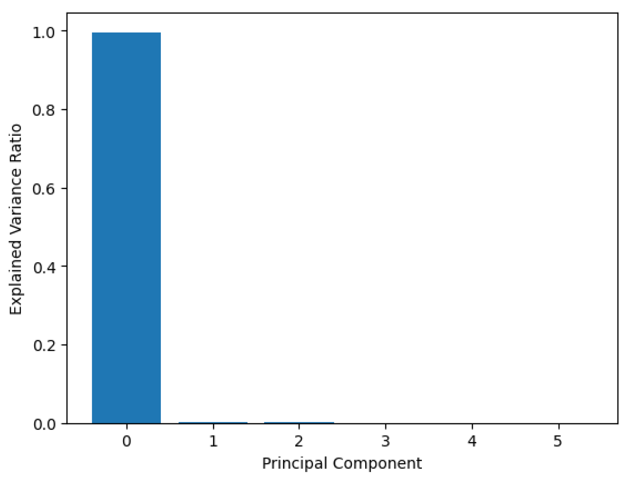
After applying the KPCA to the data, we determine the number of components that explain the main variance of the data. As shown in Figure 5, the first component explains more than 99% of the variance.
To select the relevant variables that control the polarization curve of the PEMFC and also to see which parameters have a major impact on the first component, we apply the Mutual Information method. In probability theory and information theory, the Mutual Information of two random variables is used to quantify their statistical dependence. If the variables are independent, the mutual information is zero, but it increases as their statistical dependence increases. Mutual Information is mathematically defined as follows:
  • in the discrete case:
    I ( X ; Y ) = x , y P ( x , y ) log P ( x , y ) P ( x ) P ( y ) ,
  • in the continuous case:
    I ( X ; Y ) = R R P ( x , y ) log P ( x , y ) P ( x ) P ( y ) d x d y ,
where P ( x , y ) , P ( x ) and P ( y ) are respectively the densities of ( X , Y ) , X and Y.
We apply the Mutual Information between the component that represents the data and the operating variables of the PEMFC. The variables selected by our hybrid approach are shown in Table 2.
The performance of our proposed selection technique will be compared to the other ones such as Pearson Correlation and Mutual Information (filters methods), Recursive Feature Elimination - Random Forest and Genetic Algorithm (wrappers methods), and Auto-encoder, Lasso and Ridge Regressor (embedded methods) in Section 4.

3. Model Development and Evaluation Criteria

In this section, we present how PEMFC performance can be predicted based on the relevant variables identified in the previous step using XGBRegressor and Tree-Structured Parzen Estimator (TPE). In addition, to evaluate the performance of the proposed model, evaluation criteria will be presented at the end of this section.

3.1. XGBRegressor

Extreme Gradient Boosting (XGBoost) is a library that provides an efficient implementation of the gradient boosting ensemble algorithm based on decision trees. The XGBRegressor is a special version of XGBoost designed to realize regression tasks. The objective function of XGBoost at tth iteration is defined as follows:
L ( t ) = i = 1 n l y i , y ^ i ( t 1 ) + f t x i + Ω f t ,
where l is a differentiable convex loss function, x i and y i are, respectively, the observation vector and the true value of observation i, f t is the prediction function of tree t, y ^ i ( t ) is the prediction of the observation i-th in the t-th iteration. The second term Ω is a regularization that penalizes the regression tree functions. It is defined as follows:
Ω ( f ) = γ T + 1 2 λ w 2 ,
where T is the total number of leaves in the tree, w is the leaf weights, γ and λ are hyperparameters that control the strength of the regularization.
As we can see, the function L ( t ) cannot be optimized using traditional optimization techniques in Euclidean space. So, we need to transform it into a function in the Euclidean domain. For this purpose, the second-order Taylor approximation has been applied to obtain the new form of the objective function:
L ( t ) i = 1 n l y i , y ^ ( t 1 ) + g i f t x i + 1 2 h i f t 2 x i + Ω f t ,
where g i = y ^ ( t 1 ) l y i , y ^ ( t 1 ) and h i = y ^ ( t 1 ) 2 l y i , y ^ ( t 1 ) . By removing the constant terms, we get the following simplified form in step t:
L ˜ ( t ) = i = 1 n g i f t x i + 1 2 h i f t 2 x i + Ω f t .
For more details about how to built the next learner and how to measure the quality of a tree structure, refer to [10].

3.2. Tree-Structured Parzen Estimator

The goal in this section is to estimate the hyperparameters of XGBRegressor using the Tree-Structured Parzen Estimator (TPE) [11]. For this purpose, let θ and y be respectively the hyperparameter and the loss function of the model. After choosing a new set of hyperparameters, the expectation of the improvement (EI) of the model a is given by:
E I y * ( θ ) = y * y * y p ( y θ ) d y ,
where y * is a control parameter.
To tune the hyperparameters, TPE simulates indirectly p ( y θ ) by simulating p ( θ y ) and p ( y ) . So, We replace p ( y θ ) in Equation (12) and EI becomes:
E I y * ( θ ) = y * y * y p ( θ y ) p ( y ) p ( θ ) d y ,
where p ( θ y ) is the probability density defined as piecewise function according to y:
p ( θ y ) = l ( θ ) if y < y * g ( θ ) if y y * ,
where l ( θ ) and g ( θ ) are two probability densities formed respectively by the loss values less then y * and greater than y * . So, if we consider
γ = p y < y *
we obtain
p ( θ ) = R p ( θ y ) p ( y ) d y = γ l ( θ ) + ( 1 γ ) g ( θ ) .
Furthermore, EI can be written as follows:
E I y * ( x ) = γ y * l ( θ ) l ( θ ) y * p ( y ) d y γ l ( θ ) + ( 1 γ ) g ( x ) γ + g ( x ) l ( x ) ( 1 γ ) 1 .
According to Equation (17), to determine the hyperparameters that offer the highest EI, the TPE algorithm assesses the hyperparameters using the ratio of g ( θ ) / l ( θ ) , and selects the hyperparameters θ * that yield the maximum EI.
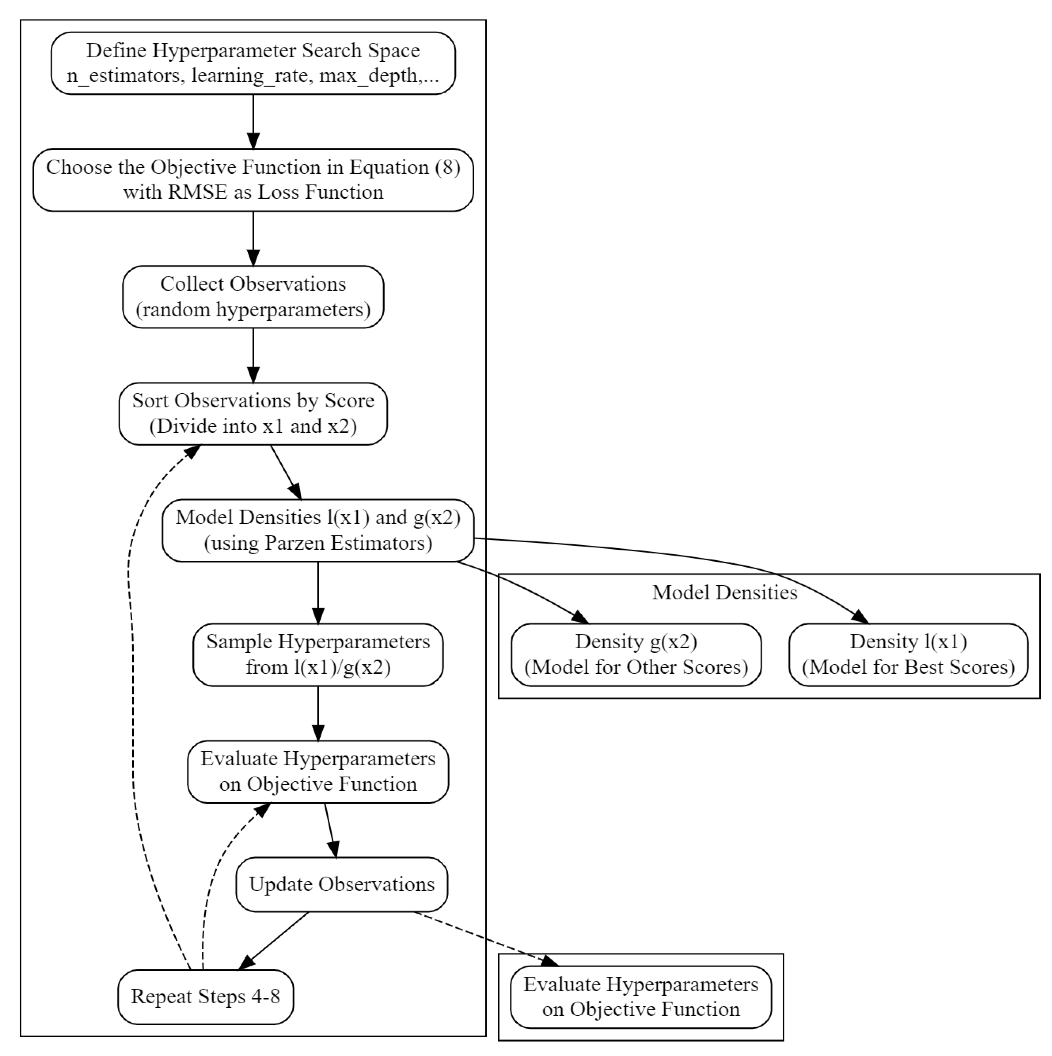
Figure 6 shows the process of estimating XGBRegressor hyperparameters using TPE.

3.3. Evaluation Criteria

To evaluate the performance of the proposed model, three measures are used: the root mean square error (RMSE), the mean absolute error (MAE), and the coefficient of determination (R 2 ). The mathematical representation of these three metrics is given below:
R M S E = 1 n i = 1 n ( V i V ^ i ) 2 .
M A E = 1 n i = 1 n | V i V ^ i | .
R 2 = 1 i = 1 n ( V i V ^ i ) 2 i = 1 n ( V i V ¯ ) 2 ,
where n is the number of observations, V i is the average PEMFC stack voltage observed, V ^ i is the predicted value, and V ¯ is the mean value of the average PEMFC stack voltage observed.

4. Results and Discussions

In this section, we apply the proposed model to predict the polarization curve based on data collected from ten different PEMFCs of different zero-emission electro-hydrogen generators. To validate and compare the performance of the proposed model, we also applied two popular machine learning regressors widely used to predict the polarisation curve: artificial neural network (ANN) and support vector machine regressor (SVR).
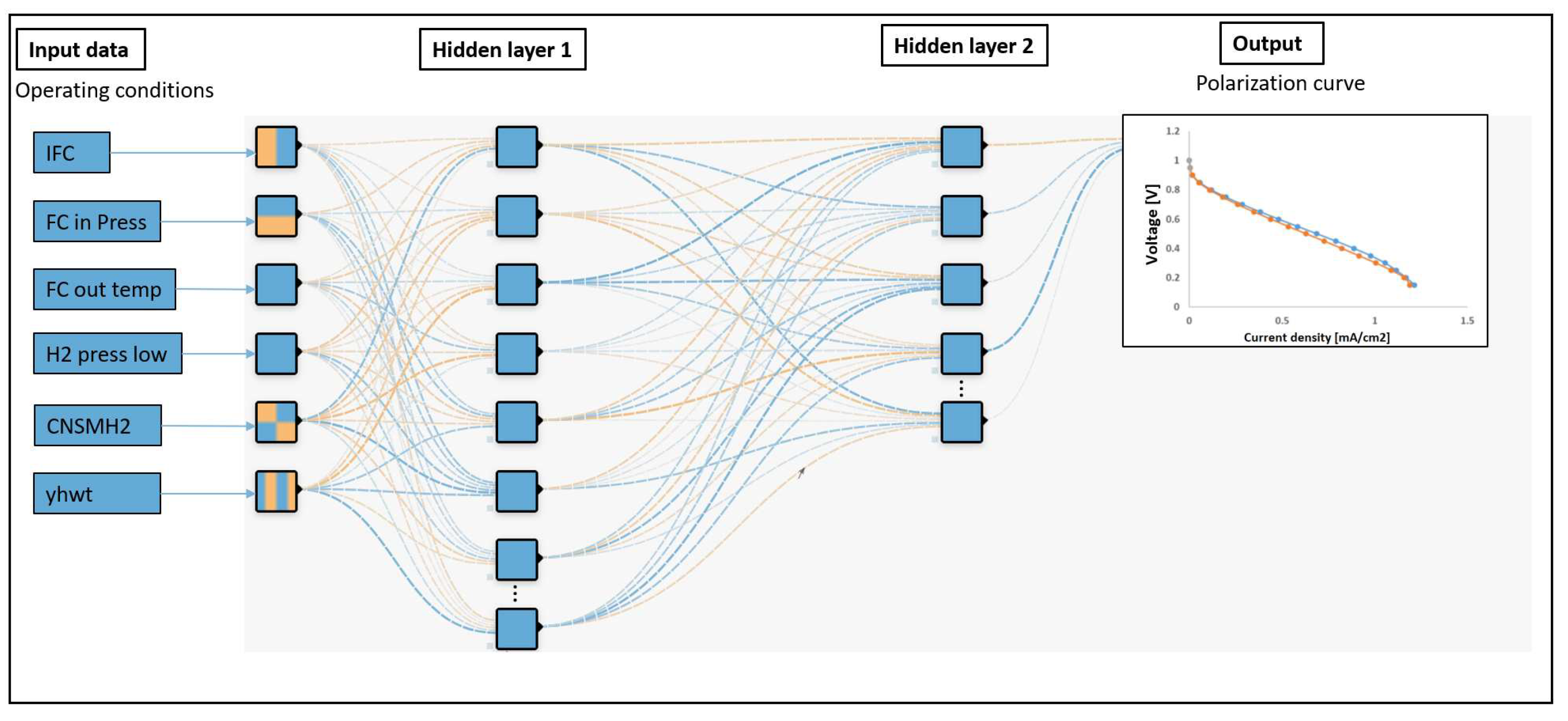
ANN is derived from biological neural networks that develop the structure of a human brain. Similar to the human brain with neurons interconnected to one another, artificial neural networks also have neurons interconnected to one another in various layers of the networks. The performance of ANN has been proven for many applications, including regression problems [17]. The defined ANN has been designed with an input layer of 6 variables, two hidden layers of 64 and 32 neurons respectively, and an output layer with a single neuron. The activation function for the first two layers is ReLU, and linear for the third layer. The chosen loss function is rmse and the Adam optimizer is used to minimize it. The training data is divided into batches of size 32 and the model is trained over 50 epochs. A schematic of the artificial neural network, where the variables selected in the previous selection are used as feature vectors (inputs) to predict the PEMFC polarization curve, is shown in Figure A1.
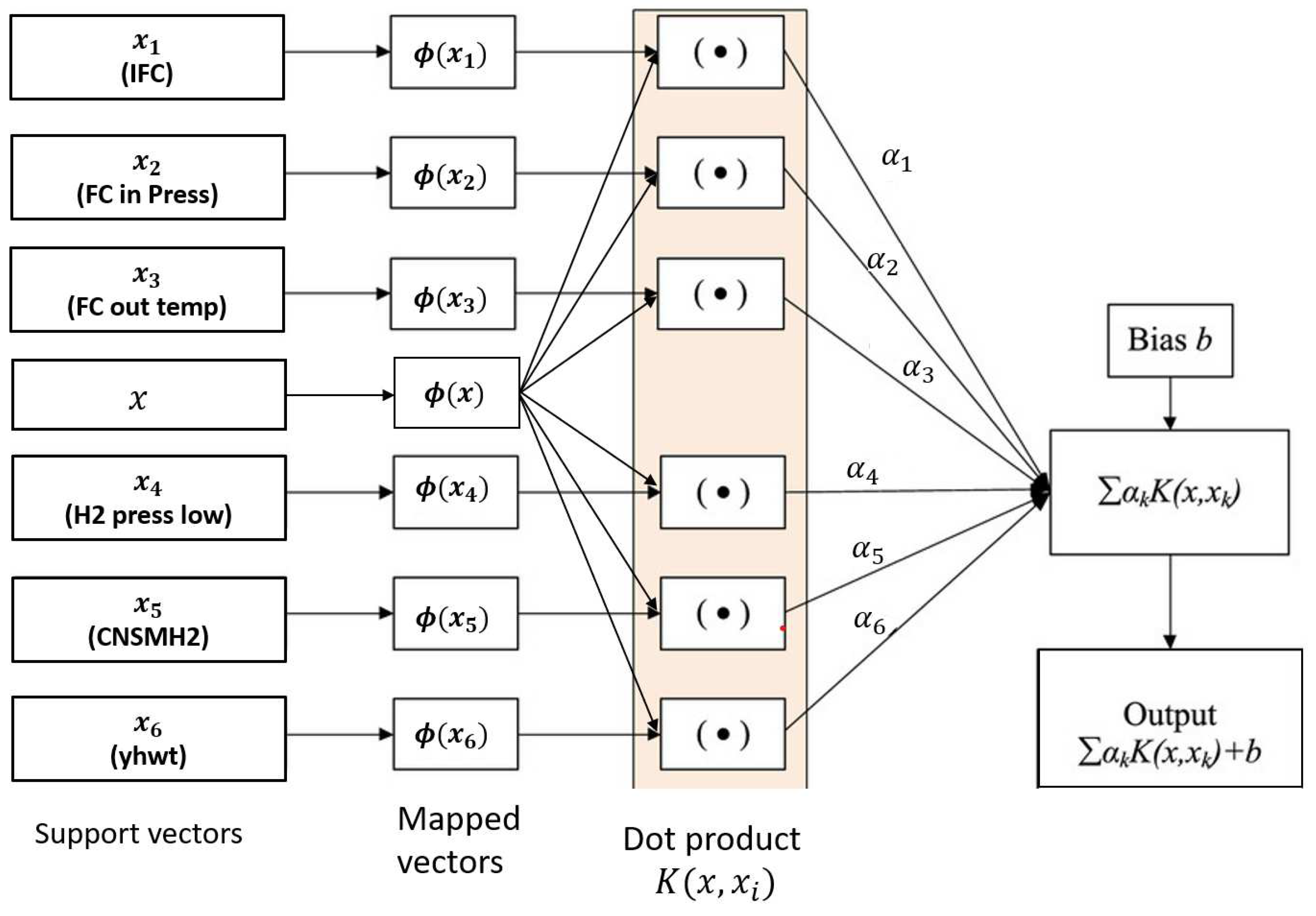
SVR is an extension of SVM applied to regression analysis [31]. It seeks to find a regression function that predicts continuous values by maximizing the margin between predictions and actual values while controlling the complexity of the model. Focuses on the data points closest to the margin, known as support vectors, to construct the regression function. SVR can use different kernel functions, like the radial basis function, to capture non-linear relationships. It solves an optimization problem that balances prediction errors and model regularization, similar to Support Vector Machines for classification. In this case, the SVR used to predict the polarization curve has a Gaussian kernel (RBF), an epsilon error tolerance of 0.025, a regularization parameter C of 5, and a kernel independent term coef0 of 0.01. Figure A1 shows a schematic of the SVR model used to predict the polarization curve of the PEMFC.
As discussed in Section 2.2.3, to better select relevant features, Kernel Principal Component Analysis and Mutual Information are jointly used. To demonstrate the effectiveness of this method, we compared it to different feature selection methods. The results of this comparison are shown in Table 3. As we can observe, the proposed feature selection method gives better results than that provided by the other methods presented in the table, and this is for both prediction models XGBRegressor and ANN.

4.1. Hyper-parameters Tuning

The different hyper-parameters of the proposed XGBRegressor model such as number estimators, max depth, learning rate, and colsample bytree were first optimized. The obtained results are reported in Table 4.

4.2. Prediction and Evaluation

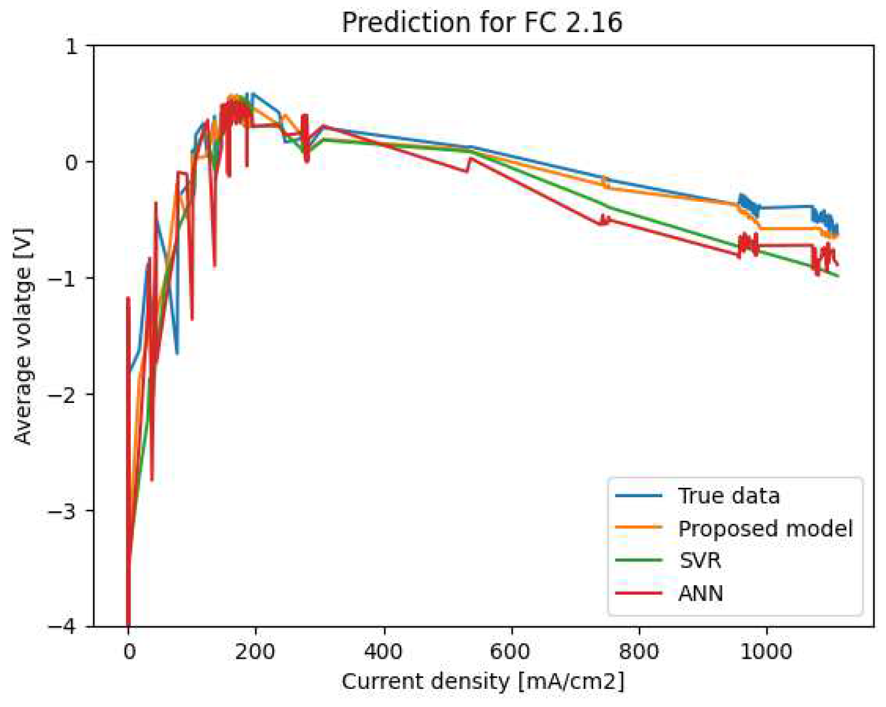
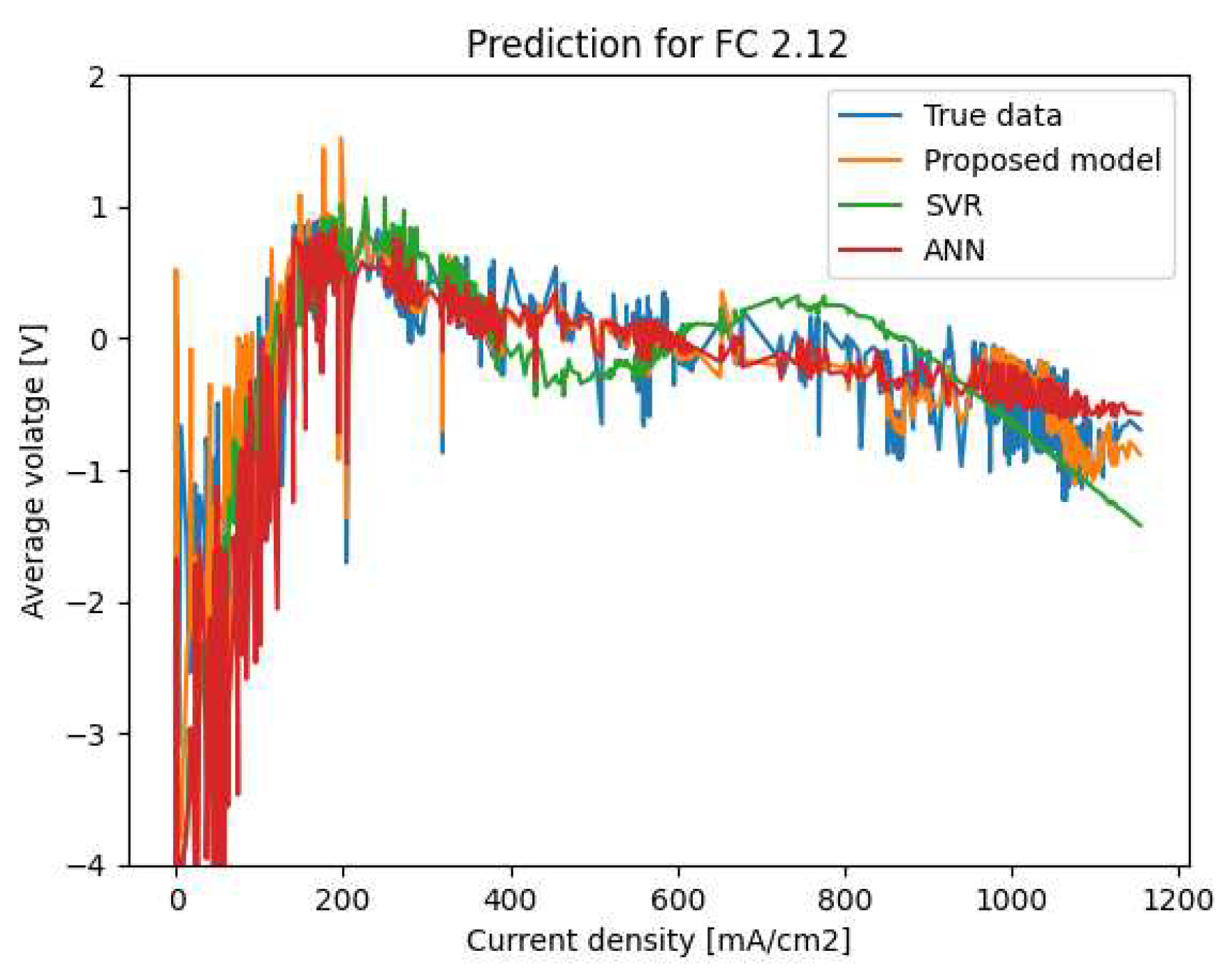
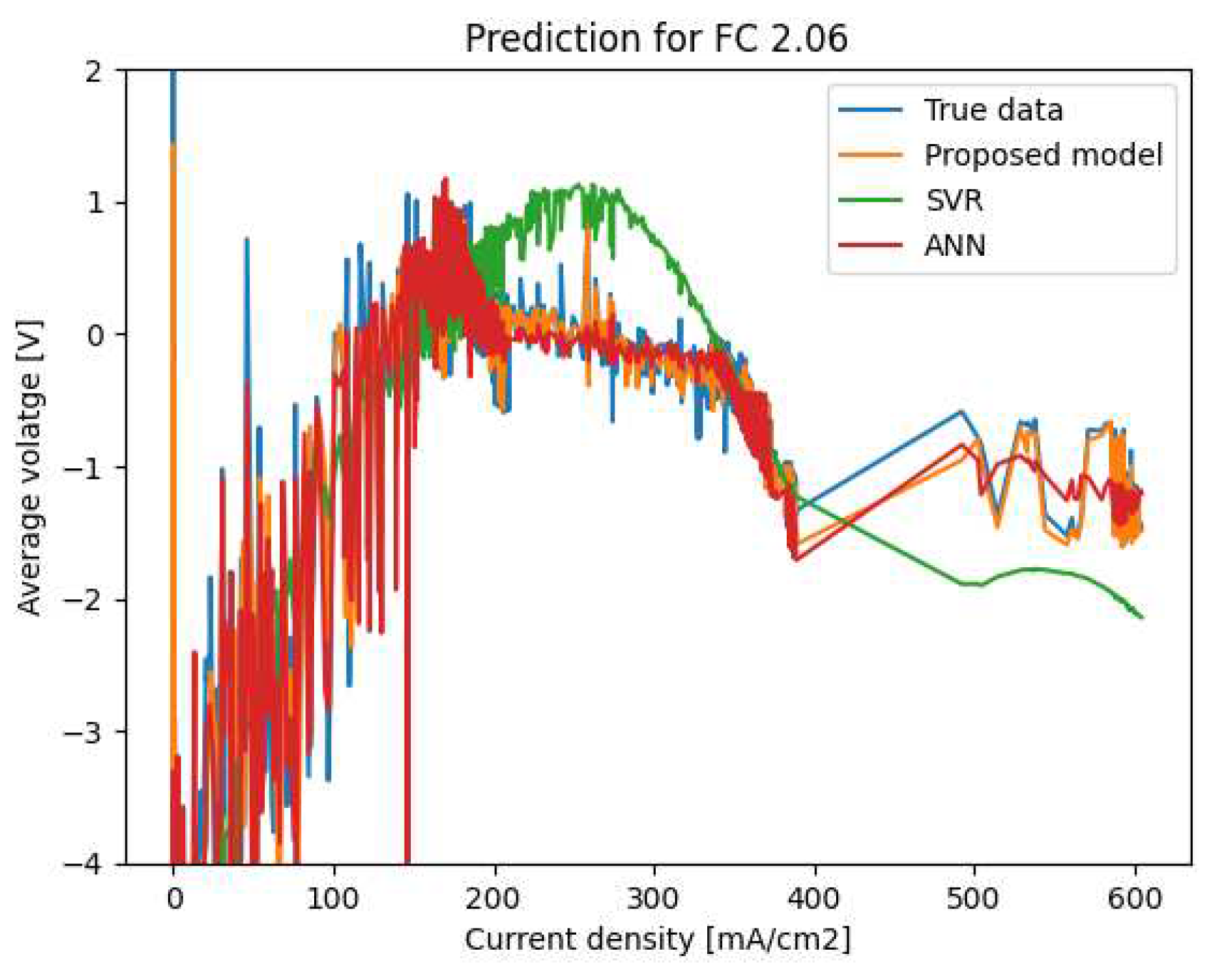
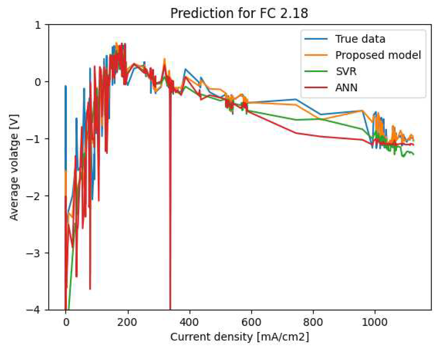
In order to validate and evaluate the quality of the proposed model, we compare its prediction results with experimental data as well as with two other machine learning models (ANN and SVR). Taking into account the operating conditions, we present the prediction results for four PEMFCs chosen to represent the ten PEMFCs. Note that each PEMFC has a serial number starting with 2. The results are shown in Figure 7, Figure 8, Figure 9 and Figure 10.
The obtained results confirm that our proposed model outperforms the ANN and SVR models. Indeed, our predicted values are close to the measured voltages, while the curves predicted by ANN and SVR are sometimes far from the real ones with significant deviations, especially in the cases of large values of the current density (greater than 200 mA/cm 2 ). We can also notice that our proposed model is more robust than ANN and SVR since its performance is always guaranteed when it is applied to the different PEMFCs.
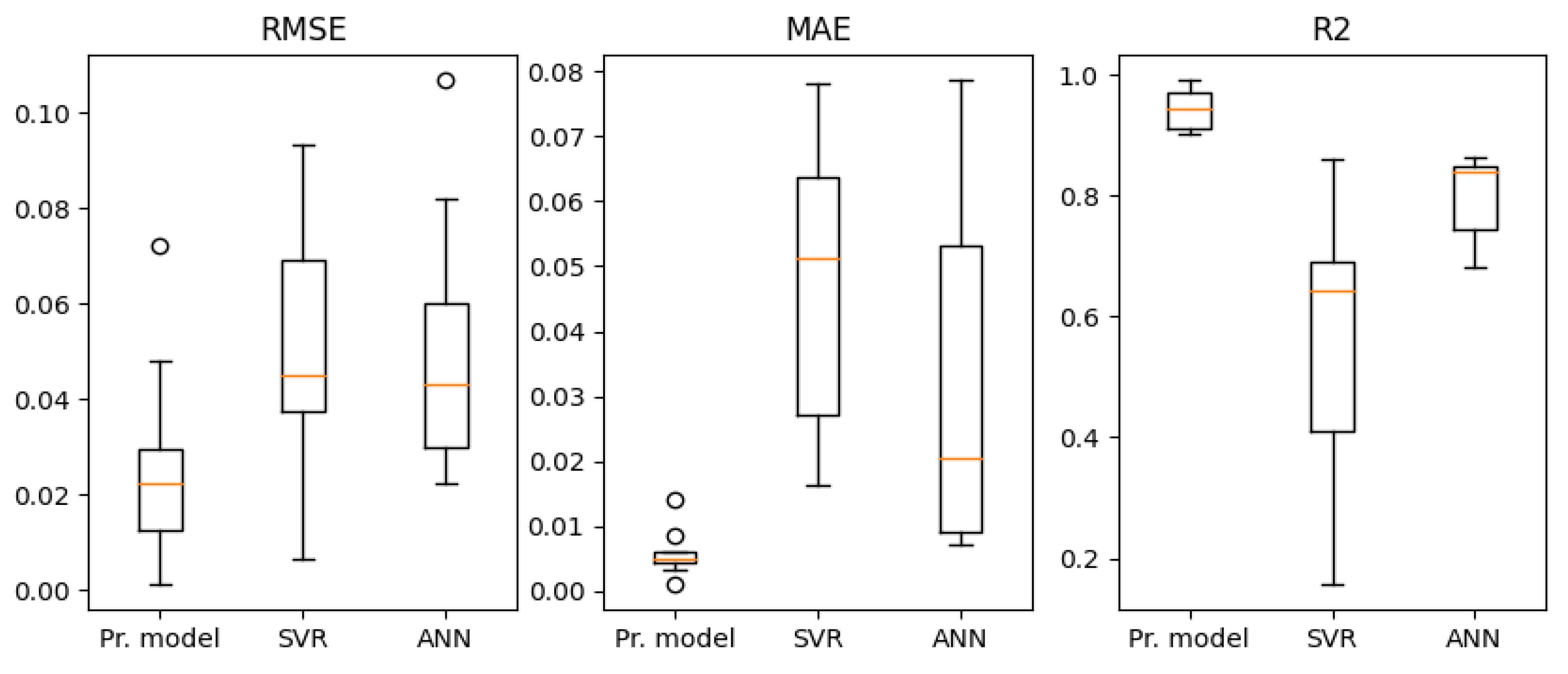
In order to estimate more precisely the performance of our model, the three evaluation metrics (RMSE, MAE, and R 2 ) were used and the obtained results are shown in Table 5. Finally, the box plots in Figure 11 are also used to reinforce our conclusions.
As we can observe from the results presented in Table 5 and Figure 11, our method always provides better results than that provided by the ANN and SVR. For example, the mean value of R2 of our method is 0.9419 , while that of SVR and ANN is only 0.5659 and 0.7987 respectively.

5. Conclusion

In this paper, a prediction approach based on the XGBRegressor with Tree-structured Parzen Estimator was proposed for estimating the PEMFC performance of electro-hydrogen generators. As PEMFCs have complex electrochemical reactions with multiple nonlinear relations between inputs (operating variables of the PEMFC) and output (average PEMFC stack voltage), a combination of Kernel Principal Component Analysis (KPCA) and Mutual Information is adopted for features selection. Through a dataset of 10 PEMFCs, the performance and effectiveness of the proposed approach in predicting the polarization curve under different operating conditions are tested and validated. In addition, when compared to two traditional models (ANN and SVR), under three performance metrics (RMSE, MAE, and R 2 ), the proposed one provides better results.

Appendix A

Appendix A.1

Figure A1. Schematic of ANN architecture for PEMFC polarization curve prediction.
Preprints 82935 g0a1
Figure A2. Schematic of SVR architecture for PEMFC polarization curve prediction.
Preprints 82935 g0a2

References

  1. Padmaja, D.L.; Vishnuvardhan, B. Comparative study of feature subset selection methods for dimensionality reduction on scientific data. IEEE 6th Int. Conf. on Advanced Computing 2016, 31–34. [Google Scholar]
  2. Zebari, R.R.; Abdulazeez, A.; Zeebaree, D.; Zebari, D.; Saeed, J. A Comprehensive Review of Dimensionality Reduction Techniques for Feature Selection and Feature Extraction. J. Appl. Sci. Technol. Trends, 2020, 01, 56–70. [Google Scholar] [CrossRef]
  3. Zebari, D.; Haron, H.; Zeebaree, S. Security Issues in DNA Based on Data Hiding: A Review. Int. J. Appl. Eng. Res., 2017, 12, 6940–6948. [Google Scholar]
  4. Dash, M.; Liu, H. Feature selection for classification. Intell. Data Anal., 1997, 1, 131–156. [Google Scholar] [CrossRef]
  5. Zhao, H.; Min, F.; Zhu, W. Cost-sensitive feature selection of numeric data with measurement errors. J. of Appl. Math., 2013, 2013. [Google Scholar] [CrossRef]
  6. Elhadad, M.K.; Badran, K.M.; Salama, G.I. A novel approach for ontology-based dimensionality reduction for web text document classification. Int. J. Software Innovation, 2017, 5, 44–58. [Google Scholar] [CrossRef]
  7. Aziz, R.; Verma, C.; Srivastava, N. Dimension reduction methods for microarray data: a review. AIMS Bioeng., 2017, 4, 179–197. [Google Scholar] [CrossRef]
  8. Wang, Q. Kernel Principal Component Analysis and its Applications in Face Recognition and Active Shape Models. arXiv preprint arXiv:1207.3538, arXiv:1207.3538.
  9. Bouchlaghem, Y.; Akhiat, Y.; Amjad, S. Feature Selection: A Review and Comparative Study. E3S Web of Conf., 2022, 351, 01046. [Google Scholar] [CrossRef]
  10. Chen, T.; Guestrin, C. Xgboost: A scalable tree boosting system. Proc. 22nd ACM SIGKDD Int. Conf. on Knowledge Discovery and Data Mining.
  11. Shen, K.; Qin, H.; Zhou, J.; Liu, G. Runoff Probability Prediction Model Based on Natural Gradient Boosting with Tree-Structured Parzen Estimator Optimization. Water, 2022, 14, 545. [Google Scholar] [CrossRef]
  12. Salva, J.A.; Iranzo, A.; Rosa, F.; Tapia, E. Experimental validation of the polarization curve and the temperature distribution in a PEMFC stack using a one-dimensional analytical model. Int. J. of Hydrogen Energy.
  13. Moreira, M.V.; Silva, G.E. A practical model for evaluating the performance of proton exchange membrane fuel cells. Renew. Energy, 2009, 34, 1734–1741. [Google Scholar] [CrossRef]
  14. Ou, S.; Achenie, L.A. A hybrid neural network model for PEM fuel cells. J. of Power Sources, 2005, 140, 319–330. [Google Scholar] [CrossRef]
  15. Zhong, Z.; Zhu, X.; Gao, G.; Shi, J. A hybrid multi-variable experimental model for a PEMFC. J. of Power Sources, 2007, 164, 746–751. [Google Scholar] [CrossRef]
  16. Lee, W.Y.; Park, G.G.; Yang, T.H.; Yoon, Y.G.; Kim, C.S. Empirical modeling of polymer electrolyte membrane fuel cell performance using artificial neural networks. Int. J. of Hydrogen Energy, 2004, 29, 961–966. [Google Scholar] [CrossRef]
  17. Han, I.; Shin, H. Modeling of a PEM fuel cell stack using partial least squares and artificial neural networks. Korean Chem. Eng. Res., 2015, 53, 236–242. [Google Scholar] [CrossRef]
  18. Zhong, Z.; Zhu, Z.; Cao, G. Modeling a PEMFC by a support vector machine. J. of Power Sources, 2006, 160, 293–298. [Google Scholar] [CrossRef]
  19. Han, I.; Chung, C.C. Performance prediction and analysis of a PEM fuel cell operating on pure oxygen using data-driven models: a comparison of artificial neural network and support vector machine. Int. J. of Hydrogen Energy, 2016, 41, 10202–10211. [Google Scholar] [CrossRef]
  20. Hong, W. Performance prediction and power density maximization of a proton exchange membrane fuel cell based on deep belief network. J. of Power Sources, 2020, 228, 154. [Google Scholar]
  21. Shen, K.; Qin, H.; Zhou, J.; Liu, G. Runoff probability prediction model based on natural gradient boosting with tree-structured parzen estimator optimization. Water, 2022, 4, 545. [Google Scholar] [CrossRef]
  22. Zheng, L.; Hou, Y.; Zhang, T. Performance prediction of fuel cells using long short-term memory recurrent neural network. Int. J. of Energy Research, 2021, 45, 9141–9161. [Google Scholar] [CrossRef]
  23. Wang, B.; Xie, B.; Xuan, J.; Jiao, K. AI-based optimization of PEM fuel cell catalyst layers for maximum power density via data-driven surrogate modeling. Energy Conv. Manag., 2020, 205, 112460. [Google Scholar] [CrossRef]
  24. Ding, R.; Wang, R.; Ding, Y.; Yin, W.; Liu, Y.; Li, J.; Liu, J. Designing AI-Aided Analysis and Prediction Models for Nonprecious Metal Electrocatalyst-Based Proton-Exchange Membrane Fuel Cells. Angew. Chem., 2020, 132, 19337–19345. [Google Scholar] [CrossRef]
  25. Legala, A.; Zhao, J.; Li, X. Machine learning modeling for proton exchange membrane fuel cell performance. Energy and AI, 2022, 10, 100183. [Google Scholar] [CrossRef]
  26. Weiwei, L. Performance prediction of proton-exchange membrane fuel cell based on convolutional neural network and random forest feature selection. Energy Conv. Manag., 2021, 243, 114367. [Google Scholar]
  27. Han, I.-S.; Chung, C.-B. A hybrid model combining a support vector machine with an empirical equation for predicting polarization curves of PEM fuel cells. Int. J. of Hydrogen Energy, 2017, 42, 7023–7028. [Google Scholar] [CrossRef]
  28. Wilberforce, T.; Olabi, A.G. Proton exchange membrane fuel cell performance prediction using artificial neural network. Int. J. of Hydrogen Energy, 2021, 46, 6037–6050. [Google Scholar] [CrossRef]
  29. Long, B.; Wu, K.; Li, P.; Li, M. A novel remaining useful life prediction method for hydrogen fuel cells based on the gated recurrent unit neural network. Appl. Sci., 2022, 12. [Google Scholar] [CrossRef]
  30. Morán-Durán, A.; Martínez-Sibaja, A.; Rodríguez-Jarquin, J.P.; Posada-Gómez, R.; González, O.S. PEM fuel cell voltage neural control based on hydrogen pressure regulation. Processes, 2019, 7, 434. [Google Scholar] [CrossRef]
  31. Zhou, Y.; Zhang, Y.; Pang, R.; Xu, B. Seismic fragility analysis of high concrete faced rockfill dams based on plastic failure with support vector machine. Soil Dyn. Earthquake Eng., 2021, 144, 106587. [Google Scholar] [CrossRef]
  32. Long, B.; Wu, K.; Li, P.; Li, M. A novel remaining useful life prediction method for hydrogen fuel cells based on the gated recurrent unit neural network. Appl. Sci., 2022, 12, 432. [Google Scholar] [CrossRef]
  33. Kheirandish, A.; Shafiabady, N.; Dahari, M.; Kazemi, M.S.; Isa, D. Modeling of commercial proton exchange membrane fuel cell using support vector machine. Int. J. of Hydrogen Energy, 2016, 41, 11351–11358. [Google Scholar] [CrossRef]
  34. Kishimoto, M.; Kishida, S.; Seo, H.; Iwai, H.; Yoshida, H. Prediction of electrochemical characteristics of practical-size solid oxide fuel cells based on database of unit cell performance. Appl. Energy, 2021, 283, 116305. [Google Scholar] [CrossRef]
  35. Talukdar, K.; Ripan, M.A.; Jahnke, T.; Gazdzicki, P.; Morawietz, T.; Friedrich, K.A. Experimental and numerical study on catalyst layer of polymer electrolyte membrane fuel cell prepared with diverse drying methods. J. of Power Sources, 2020, 461, 228169. [Google Scholar] [CrossRef]
  36. Danilov, V.A.; Tade, M.O. An alternative way of estimating anodic and cathodic transfer coefficients from PEMFC polarization curves. Chem. Eng. J., 2010, 156, 496–499. [Google Scholar] [CrossRef]
  37. Kim, J.; Lee, S.M.; Srinivasan, S. Modeling of proton membrane fuel cell performance with an empirical equation. J. Electroanal. Chem., 1995, 142, 2670–2674. [Google Scholar] [CrossRef]
  38. Guinea, D.M.; Moreno, B.; Chinarro, E.; Guinea, D.; Jurado, J.R. Rotary-gradient fitting algorithm for polarization curves of proton exchange membrane fuel cells (PEMFCs). Int. J. Hydrogen Energy, 2008, 33, 2774–2782. [Google Scholar] [CrossRef]
  39. Bressel, M.; Hilairet, M.; Hissel, D.; Bouamama, B.O. Extended Kalman filter for prognostic of proton exchange membrane fuel cell. Appl. Energy, 2016, 164, 220–227. [Google Scholar] [CrossRef]
  40. Wang, Y.; Wu, K.; Zhao, H.; Li, J.; Sheng, X.; Yin, Y.; Jiao, K. Degradation prediction of proton exchange membrane fuel cell stack using semi-empirical and data-driven methods. Energy and AI, 2023, 11, 100205. [Google Scholar] [CrossRef]
  41. Hu, Y.; Zhang, L.; Jiang, Y.; Peng, K.; Jin, Z. A hybrid method for performance degradation probability prediction of proton exchange membrane fuel cell. Membranes, 2023, 13, 426. [Google Scholar] [CrossRef]
  42. Pan, R.; Yang, D.; Wang, Y.; Chen, Z. Performance degradation prediction of proton exchange membrane fuel cell using a hybrid prognostic approach. Int. J. of Hydrogen Energy, 2020, 45, 30994–31008. [Google Scholar] [CrossRef]
  43. Zhou, D.; Al-Durra, A.; Zhang, K.; Ravey, A.; Gao, F. Online remaining useful lifetime prediction of proton exchange membrane fuel cells using a novel robust methodology. J. of Power Sources, 2018, 399, 314–328. [Google Scholar] [CrossRef]
  44. Cheng, Y.; Zerhouni, N.; Lu, C. A hybrid remaining useful life prognostic method for proton exchange membrane fuel cell. Int. J. of Hydrogen Energy, 2018, 43, 12314–12327. [Google Scholar] [CrossRef]
  45. Chen, K.; Laghrouche, S.; Djerdir, A. Aging prognosis model of proton exchange membrane fuel cell in different operating conditions. Int. J. of Hydrogen Energy, 2020, 45, 11761–11772. [Google Scholar] [CrossRef]
  46. Wilberforce, T.; Olabi, A.G. Proton exchange membrane fuel cell performance prediction using artificial neural network. Int. J. of Hydrogen Energy, 2021, 46, 6037–6050. [Google Scholar] [CrossRef]
  47. Zuo, J.; Lv, H.; Zhou, D.; Xue, Q.; Jin, L.; Zhou, W. .. & Zhang, C. Deep learning based prognostic framework towards proton exchange membrane fuel cell for automotive application. Appl. Energy, 2021, 281, 115937. [Google Scholar]
  48. He, K.; Liu, Z.; Sun, Y.; Mao, L.; Lu, S. Degradation prediction of proton exchange membrane fuel cell using auto-encoder based health indicator and long short-term memory network. Int. J. of Hydrogen Energy, 2022, 47, 35055–35067. [Google Scholar] [CrossRef]
  49. Legala, A.; Zhao, J.; Li, X. Machine learning modeling for proton exchange membrane fuel cell performance. Energy and AI, 2022, 10, 100183. [Google Scholar] [CrossRef]
Figure 1. (EODev): zero-emission electro-hydrogen generator.
Preprints 82935 g001
Figure 2. Process of feature selection.
Preprints 82935 g002
Figure 3. Process of feature extraction.
Preprints 82935 g003
Figure 4. Process of PEMFC features selection.
Preprints 82935 g004
Figure 5. KPCA results: explained variance per component.
Preprints 82935 g005
Figure 6. Process of estimating XGBRegressor parameters using TPE.
Preprints 82935 g006
Figure 7. Polarization curve prediction for FC 2.16.
Preprints 82935 g007
Figure 8. Polarization curve prediction for FC 2.12.
Preprints 82935 g008
Figure 9. Polarization curve prediction for FC 2.06.
Preprints 82935 g009
Figure 10. Polarization curve prediction for FC 2.18.
Preprints 82935 g010
Figure 11. Box-plot of the three models in term of RMSE, MAE and R 2 .
Preprints 82935 g011
Table 1. Operating variables of the PEMFC.
Variable Description Unit
VFC Average PEMFC stack voltage V
IFC PEMFC stack current A
ACP Inv Temp Air compressor inverter temperature °C
ACP Mot Temp Air compressor internal temperature °C
Air comp speed Air compressor speed rpm
Air Flow PEMFC air flow rpm
CNSMH2 Instantaneous H2 consumption mg
f4g fwctrvo ratrvnw 3 way valve opening rate %
FC in Press PEMFC input air pressure kPa
FC out temp PEMFC output temperature °C
FCO TEMP Output coolant temperature °C
H2 mean pressure Hydrogen pressure middle Kpa
H2 press low H2 pressure at PEMFC inlet kPa
H2 press target H2 pressure target in PEMFC kPa
HP pump speed H2 pump speed rpm
MES FC PEMFC net output power W
MOD FC PEMFC mode -
Rad out temp Radiator output temperature °C
REVAPREF Air compressor speed control rpm
Water pump spd Water pump speed rpm
Water pump spd req Water pump speed request rpm
yhwt Coolant Temperature °C
Table 2. Selected variables with the proposed method.
Variable Description
IFC PEMFC stack current
FC in Press PEMFC input air pressure
FC out temp PEMFC output temperature
H2 press low H2 pressure at PEMFC inlet
CNSMH2 Instantaneous H2 consumption
yhwt Coolant Temperature
Table 3. Results of the different feature selection methods in terms of RMSE and R 2 , with k represents the number of features selected.
XGBRegressor ANN k
RMSE R 2 RMSE R 2
Filter method Mutual Information 0.0501 0.8717 0.0588 0.7354 4
Correlation 0.1065 0.5919 0.1633 0.5615 7
Wrapper method RFE-Random Forest 0.0490 0.8909 0.0550 0.7312 9
Genetic algorithm 0.0914 0.7590 0.0766 0.6918 12
Embedded method Auto-encoder 0.0431 0.8984 0.0549 0.7422 8
Lasso 0.0652 0.8577 0.0789 0.6700 13
Ridge 0.0682 0.8505 0.0734 0.6692 9
Proposed method 0.0476 0.9233 0.0537 0.7689 6
Table 4. Estimation of Hyper-parameters in the proposed XGBRegressor model.
Hyper-parameters Description Estimated value
n_estimators number of decision trees to be created 1500
max_depth the maximum depth of each decision tree 5
learning_rate the rate at which the model learns from the data 0.01
colsample_bytree the fraction to be used for training each tree 0.060
loss function RMSE -
Table 5. Polarization curve results of the three methods in terms of RMSE, MAE and R 2 .
Proposed model SVR ANN
RMSE MAE R 2 RMSE MAE R 2 RMSE MAE R 2
FC 2.21 0.0100 0.0050 0.9758 0.0350 0.0215 0.6015 0.0424 0.0172 0.8351
FC 2.19 0.0220 0.0062 0.9512 0.0374 0.0162 0.8602 0.0410 0.0134 0.8476
FC 2.18 0.0280 0.0085 0.9500 0.0707 0.0641 0.6625 0.0435 0.0641 0.8417
FC 2.17 0.0194 0.0047 0.9071 0.0373 0.0267 0.6228 0.0236 0.0071 0.8483
FC 2.16 0.0480 0.0141 0.9060 0.0932 0.0781 0.6622 0.0632 0.0236 0.8446
FC 2.14 0.0053 0.0034 0.9809 0.0500 0.0433 0.2825 0.0507 0.0307 0.7236
FC 2.13 0.0011 0.0010 0.9904 0.0064 0.063 0.3480 0.0821 0.0606 0.6987
FC 2.12 0.0720 0.0049 0.9021 0.0921 0.0689 0.7629 0.1068 0.0786 0.6810
FC 2.08 0.0230 0.0044 0.9192 0.0640 0.0593 0.1560 0.0223 0.0076 0.8024
FC 2.06 0.0300 0.0055 0.9367 0.0400 0.0280 0.7012 0.0264 0.0076 0.8640
Mean 0.0258 0.0057 0.9419 0.0526 0.0469 0.5659 0.0502 0.0310 0.7987
Disclaimer/Publisher’s Note: The statements, opinions and data contained in all publications are solely those of the individual author(s) and contributor(s) and not of MDPI and/or the editor(s). MDPI and/or the editor(s) disclaim responsibility for any injury to people or property resulting from any ideas, methods, instructions or products referred to in the content.
Copyright: This open access article is published under a Creative Commons CC BY 4.0 license, which permit the free download, distribution, and reuse, provided that the author and preprint are cited in any reuse.
Prerpints.org logo

Preprints.org is a free preprint server supported by MDPI in Basel, Switzerland.

Subscribe

© 2024 MDPI (Basel, Switzerland) unless otherwise stated