
Submitted:
21 August 2023
Posted:
23 August 2023
You are already at the latest version
Abstract
In this work, the nearest neighbor distances and Voronoi cell features of the Cu-Ag deposits were analyzed and fitted with Lognormal, Weibull, and Gamma distributions. The nearest neighbor distance distributions of the samples were compared with those of complete spatially random points, showing spatial inhomogenity due to the nucleation exclusion effect. The radial distribution function was calculated, showing both influences from the grain size and the nucleation exclusion effect. Voronoi cells were generated based on the shape of the grains. The size, occupancy, and coordination of the Voronoi cells were examined and fitted. The results show that despite the Cu-Ag deposits seem to be governed by instantaneous nucleation mode, the spatial distribution of the nuclei is more impacted by the nucleation exclusion effect than the Cu-only samples. This behavior is also justified by the grain size distribution generated with Voronoi cell size and occupancy distributions.
Keywords:
Electrodeposition
; Nucleation and growth
; Particle statistics
; Lognormal
; Weibull
; and Gamma distributions
1. Introduction
Potentiostatic transient at the onset of electrodeposition is frequently modeled by the Classical model (1968) and the Scharifker-Hills model (S-H model, 1983) of nucleation/growth [1,2]. Despite this derivation is quite simple, widespread and successful in explaining the potentiostatic transients at the initial stage of electrodeposition, microstructural evidence of the fundamental assumptions of the S-H model is not sufficient [3]. For example, Ustarroz et al. reported that Pt particles were mainly grown through clustering of newly formed Pt nuclei (called secondary nucleation [4]) during electrodeposition of Pt at carbon-coated TEM grids. These potentiostatic transients imply significant deviations from the physics of S-H model [5]. Since the fundamental assumptions of the S-H model express a specific scenario of nucleation and growth, we believe that analyzing the statistical features of the grains at the initial stage of electrodeposition could offer useful insights on the S-H model.
Despite the distributions of features in electrodeposited grains have been observed [6], the relation between the nucleation modes from the S-H model and the grain statistics is rarely investigated from a morphological aspect (despite frequently referred in explaining the potentiostatic transients [3]). So far, the only systematically examined statistics features of electrodeposited grains are the particle sizes the nearest neighbor distances [7,8]. The diffusion fields around the particles formed at early time will reduce the nucleation rate around those particles; such behavior is usually referred to as nucleation exclusion effect. The area with very low nucleation rate around a single grain is its nucleation exclusion zone.
The impact of nucleation exclusion zones on the randomness of the spatial distribution of the nuclei has been observed in various works, reflected by the distribution of the nearest neighbor (NN) distances and the radial distribution function (RDF) of the nuclei [9,10,11,12,13]. Experimental results show that the degree of inhomogeneity could be influenced by the deposition overpotentials [10] and the supporting electrolyte [14]: increasing the overpotential reduces the NN distances and undermine the randomness of the nuclei, while addition of the supporting electrolyte will improve the spatial randomness of the nuclei. The impact of nucleation exclusion zones in different systems can be different. For instance, the exclusion effect can extend to the 15th nearest neighbor of the Pb particles at vitreous carbon substrate [10], but only to the 2nd NN of the Ag grains at boron-doped diamond electrodes [15]. The nucleation events in electrodeposition could last from seconds to tens of seconds, based on direct observation of the nuclei with optical microscopes [14,15,16].
Recently, Moehl et al. (2020) observed the in-plane periodicity of Au particles electrodeposited at Si substrate using grazing incidence small-angle X-ray scattering (GISAXS) with synchrotron X-ray [17]. To separate the effect of the nucleation kinetics and growth kinetics on the final deposit, a double-pulse deposition is used [14]. A small XRD peak, corresponding to periodicity (correlation distance) slightly larger than the nearest neighbor distances of the grains, was observed in the horizontal diffraction profile (along the substrate). Moehl et al. considered the correlation distance corresponds to the periodicity of larger particles, instead of all particles [17].
Besides the experiments, various simulation efforts were conducted to mimic such inhomogeneity. In 1992, Scharifker et al. proposed the method of simulating the nucleation and growth process with progressive and nucleation modes of the S-H model, in which the instantaneous nucleation mode leads to completely spatially random grains while the nucleation exclusion zone during the progressive nucleation significantly impacted the spatial homogeneity of the grains [18]. With experimentally measured nucleation rate from the potentiostatic transients [10], Mostany et al. simulated the spatial distribution of grains (RDF and NN distances) from the nucleation process under the influence of nucleation exclusion zones (with radius ), showing good agreement between observed and simulated results (1st-15th NN neighbors) [9,10]. In addition to Scharifker’s approach with hard-cored nucleation exclusion zones, Milchev et al. [7], Kruijt et al. [14], Hyde et al. [15], and Tsakova and Milchev [19] simulated the impact of diffusion fields at a given sites with diffused hemispherical diffusion fields from its 1st nearest nucleus [7,14,15,19] or n-th (n<5) nearest nuclei [14], showing good agreement with observed values. Simulations by Tsakova and Milchev showed that inhomogeneity increases with nucleation site density [19]. Those works, however, did not connect their simulated results with an analytical solution of their model, nor compared with the distributions for spatial features in metallurgy.
To the best of our knowledge, a qualitative understanding between the deposition conditions and the spatial distribution of the deposit is still lacking. The hard-disk model developed by Torquato et al. offers analytical solution to the nearest neighbor distance distribution in a system consist of impenetrable disks with the same diameter, which cannot describe the distributions in electrodeposition systems [20]. Recently, rooted on the Kolmogorov-Johnson–Mehl–Avrami (KJMA) approach, Tomellini at al. proposed a theory for estimating the RDF and NN distance distribution of nuclei generated at a constant nucleation rate (progressive nucleation) under the influence of nucleation exclusion zones (following a generalized growth law of ) [21]. This model suggests that the 1st NN distances could be fitted by a generalized Gamma distribution. However, from our perspective, how to use this model to explain the statistics of the spatial features in actual deposits is still very obscure. Developing an analytical theory for a nucleation and growth model in electrodeposition beyond the S-H model is still an ongoing investigation [5,8,22], with Politi and Tomellini categorized the strategies of these theories in two fashions: “3D nucleation and growth” or “planar diffusion analogy” [8].
The distributions functions (for example, Lognormal, Weibull and Gamma distributions) reflect the underlying mechanism of nucleation and growth during material processing [23]. Regarding electrodeposition, knowing such a mechanism is important to understand the transition between the initial deposit and the lateral growth under steady-state deposition. Thus, in this work, we attempt to compare the observed spatial features in electrodeposited Cu or Cu-Ag particles with the Lognormal, Weibull, and Gamma distributions, in a hope that a theory about the spatial distributions in electrodeposited particles could be proposed in the future.
2. Experiments
The scanning electron microscopy (SEM) images used in this paper is from the dataset of our previous works [24,25,26]. Heavily As-doped H-terminated n-Si(001) wafer with resistivity < (Silicon Quest International) was cut, then cleaned by methylene chloride, acetone, and ethanol. The n-Si(001) pieces were then etched in 30% HF solution and soldered by In-Ga (at room temperature) at metal supports. The depositions were conducted in a typical 3-electrode cell, with 300mL beaker as the container, Pt mesh as the anode, n-Si pieces of ~1cm2 as substrate, saturated mercurous sulfate (SMSE, 0.64 vs. SHE) as the reference electrode, and EG&G PAR 273 potentiostat/galvanostat as the potentiostatic control. The deposition bath is associated with components of 10mM CuSO4 + 0.5M H2SO4 + 0, 0.1, or 1mM AgNO3. No stirring during the deposition, and the n-Si(001) substrates were exposed to surrounding illuminations during deposition. The cutoff deposition time for all samples is 5 seconds. The SEM images were collected with JEOL JSM-6700F field emission scanning electron microscope (FE-SEM).
The spatial features in the SEM images (Figure 1) were processing with conducted using ImageJ [6]. The Voronoi cells were generated based on the shapes of the grains, instead of the weight center of the grains. On the other hand, the n-th rank NN distances were generated based on the weight center of the grains. To avoid the interference from the edges of the imaging area, a cut-off distance with the maximum observed distance of given rank of NN distances were used: only the grains outside this cutoff distance were used for the NN distance distribution. The radial distribution function (RDF) was calculated using a fixed 500nm cut-off distance, since the range of interest is about 500nm.
3. Fitting Functions
3.1. Generalized Gamma Distribution
Spatial characteristics of a grain structure often reflect to the nucleation and growth behavior of the system [23]. Distributions derived from the Generalized Gamma distribution, such as Gamma, Lognormal and Weibull distributions, are frequently used for the statistics of the features of a grain structure [23,27].
The Generalized Gamma distribution is the analytical result for the distributions of -th nearest neighbor distance for a set of completely randomly located points. With as the spatial density of the points, the probability of -th nearest neighbor with a length in an -dimension space is a generalized Gamma function of , , and [7,28]:
Note that for 2D scenario . The mean and standard deviation of this distribution is: and .
1When nucleation exclusion zone is significant, the spatial distribution of the center of grains will no longer be homogeneous [18,29]. To the best of our knowledge, Tomellini’s model (2017) is the only analytical model on the spatial distribution of electrodeposited particles.
For electrodeposition, Tomellini’s model assumes that (1) nucleation rate is a constant (progressive mode), and (2) the radius of the nucleation exclusion zone . With those physical setups, Tomellini found that the 1st NN distance distribution, after full coalescence of the nucleation exclusion zones, is a Generalized Gamma distribution with and . However, Tomellini’s model only introduced two of the three fitting parameters – this model did not discuss how to calculate the mean 1st NN distance based on a certain definition of nucleation exclusion zone with parameters from to the mass-transport and nucleation kinetics of actual electrodeposition.
In addition to the NN distance distribution, the Generalized Gamma distribution is closely related to the particle size distribution of a system. The 2-parameter Weibull distribution is achieved from Generalized Gamma function with , and Gamma distribution is achieved with . Meanwhile, the lognormal distribution is proven to be a special case of Generalized Gamma distribution when [30,31,32]. Therefore, the Generalized Gamma distribution could be used to choose the distribution functions for a given set of particle sizes. However, how does the Generalized Gamma distribution connect with the physical model of the evolution of particles is still unclear to us [33]. Arbitrarily fitting the data with the Generalized Gamma distribution is difficult [30,31,32]. Thus, the Generalized Gamma distribution is difficult to be used to analyze particle size distribution.
3.2. Weibull Distribution - Size of Fragments with Randomly Partitioned Volumes
According to Rinne [34], several physical models are derived from the Weibull distribution: (1) the weakest link model: the failure probability of the entire system due to the failure of the weakest (or shortest lifetime) part of the entire system [34]; (2) degradation process, if the first passage time of the failure for individual part follows inverse Gaussian distribution; (3) hazard rate regarding the wearing of a device; and (4) the “generalized broken stick model”: the sizes distribution of broken pieces of a finite length stick with an expected size [27,35]. With fitting parameters , the expression of the Weibull distribution of is:
Note that the fit from the Weibull distribution is independent of how the particle shape is defined. Assuming a particle with volume , both and is incorporated into the fits parameters without changing the shape of the fitted curve.
Lourat (1974) derived that the radius of particles fulfilled a Weibull distribution with [36] (which is also called “Rayleigh distribution” [23]). Fayad et al. simulated the grain evolution during an annealing process in a 2D system, leading to a Weibull distribution of grain radius R with at the steady state [37].
In an analogy to the generalized broken stick model [38], the Weibull distribution could relate to the allocation of depositing species to each nucleus. When the allocation of resources is completely random, with the volume of each particle as the variable of the distribution, the fitting parameters and . On the other hand, when the particle radius is completely random, the particle size could be described by the Weibull distribution, with for and for . Figure B1 in Appendix B demonstrates the said process. However, the physical picture of the Weibull distribution in the nucleation and growth problem is still unclear to us, and there could be other explanations for the occurrence of Weibull distribution.
3.3. Lognormal Distribution – Law of Proportionate
The lognormal distribution [39,40,41,42,43,44,45] is frequently used in generalized nucleation-growth statistics (e.g., bacteria population [46]; shape and size of metallurgical grains [47], colloids [48], cumulus clouds [49]; pore sizes in soils [50]; commercial firm sizes [51], or clumping of galaxies [52]), also some other aspects such as survival time [53], paper citations [54], surgical procedure duration [55], or user post length in Internet discussions [56].
Conceptually, the Lognormal distribution will emerge when the values of original random events evolve with respect to steps by multiplied with a series of random parameters. With fitting parameters , the expression of the Lognormal distribution of particle size is:
Note that the fitting of Lognormal distribution is independent of how the particle shape is defined. If fulfills Lognormal distribution of variables , then fulfills Lognormal distribution of .
According to the book by Aitchison and Brown in 1966 [45], the Lognormal distribution for grain size of grinded material was firstly proposed by Kolmogoroff (1941), who assumed the partition of each particle being independent of their size at discrete breakage steps and the step number [57,58]. A continuous version of this model associated with a breakage frequency was recently (2003) proposed by Gorokhovski and Saveliev regarding the breakage of liquid droplets (initially of size ) produced by air-blast [59]. In 2008, Bergmann and Bill showed that when the untransformed fraction of the parent phase is proportional to , with a constant nucleation rate and growth rate , the grain sizes at the end of transformation will be similar to the Lognormal distribution [60,61]. Despite the assumption on the observed nucleation rate in their work agrees with the apparent nucleation rate for the progressive nucleation mode of S-H model [62], it is uncertain whether the initial electrodeposits could be expressed with this model (which was derived for grain statistics in complete crystallization).
In terms of electrodeposition, the Lognormal distribution could be achieved for grains initially at the same size when (1) the average growth & shrink rate of each grain is proportional to its size () but independent of deposition time, and (2) the randomness of the growth & shrink is independent of the size of the grains and deposition time [63,64]. A hypothetical scenario is given in Figure B2 in Appendix B. However, the relationship between the Lognormal distribution and the electrodeposition problem is still unknown, and there could be other explanations for the occurrence of Lognormal distribution.
3.4. Gamma Distribution – Size of Voronoi Cells with Completely Randomly Located Points
The Gamma distribution is known to be closely related to the statistics of events fulfilling Poisson distribution [65]. With fitting parameters , the expression of the Gamma distribution is:
Where means the volume of the particles at given dimension (e.g., for 2D circular plates). Note that the fitting results will be different if the particle shape is defined differently.
The size distribution of the Voronoi cells () associated with completely spatially random points (generated from homogeneous Poisson point process), called Poisson-Voronoi tessellation, could be described by the Gamma distribution [66,67]. In this case, the fitting parameter could be separated into , with as the density of the random points. While the 1D scenario of the tessellation analytically fulfills a Gamma distribution, the scenarios at higher dimensions are not analytically available but empirically successful: for 1D system, for 2D system, and for 3D system [66,67]. An example of the 2D system is shown in Figure B3 in Appendix B. In other aspects, Gamma distribution could also be derived as the probability for at least random events happening between time and [65].
In summary, the Gamma distribution is strongly associated with the grain size with a Poisson-Voronoi nucleation/growth model. In other words, if the centers of grains at given time are randomly distributed across the entire volume, the size distribution of the Voronoi cells generated from these points are expected to be fitted with Gamma distribution [68]. However, the Gamma distribution connected to electrodeposition is still unknown, and there could be other explanations for the occurrence of Gamma distribution.
3.5. Fitting with Gamma, Lognormal and 2-Parameter Weibull Distributions
Before defining the parameters in the fitting functions, we should define the average value of the grain area and other properties. The mean grain size is averaged based on the radius of the grains (), instead of the area of grains:
All the fittings were conducted using the cumulative distribution function (CDF) of each distribution, since the choice of bin size might impact the fitting results with the probability density functions (PDFs). For more details about the applications, PDFs, and physical pictures of the Generalized Gamma distribution, the Lognormal distribution, the Weibull distribution, and the Gamma distribution, a short commentary is given in Appendix B. Example of fitting the particle size with CDF is shown in Appendix C.
Regarding the cumulative distribution function (CDF) of the Lognormal distribution for feature , with two fitting parameters (, ), we have:
Regarding the CDF of the Weibull distribution for feature , with two fitting parameters (, ), we have:
Regarding the CDF of the Gamma distribution for feature , with two fitting parameters (, ), we have:
Note that is the average radius of the grains, whereas is the average area of the grains. We will use their CDF functions to fit the radii derived from the observed areas (assumed to be circular particles) from the SEM images.
3.6. Behavior of the Fittings
By defining the fitting parameter based on the average values of the observed distributions for the Lognormal and Weibull distributions, we should expect . The mean values of Lognormal and Weibull distributions based on our definitions could be calculated as:
Since the fitted parameter is large for both Lognormal and Weibull distributions, and is closer to the value of 1. Successful fitting requires that the mean of the fitted distribution function is very close to the mean value of the original dataset (). Therefore, the fitted parameters are very close to the value of 1.
Regarding the Gamma distribution, both fitting parameters have similar fitted values. Considering the mean value of Gamma distribution:
Since successful fitting requires the mean of the fitted function is very close to the mean of the observed distribution, for successful fittings with Gamma distribution.
For some of the fitting results, the Gamma distribution fitting result seems to be in the middle of Lognormal and Weibull fitting results. The Gamma, Lognormal and Weibull distributions are all derived from the Generalized Gamma distributions. To examine the relationship between those distributions in the fittings, fittings of the distributions of particle size and nearest neighbor distance in different orders () will be used as examples (Figure 2).
The data in Figure 2a could be fitted with the Lognormal distribution. By decreasing the order in the definition of the particle size, the Gamma distribution behaves more like the Lognormal distribution fitting results. In other words, the fitting parameters of the Gamma distribution is very large (e.g., values of 12 or even 30), the fitted distribution behaves like the Lognormal distribution.
The data in Figure 2b agrees well with the Weibull distribution. By increasing the order in the definition of the nearest neighbor distance, the Gamma distribution behaves more like the Weibull distribution results (especially when ). It also means that if the fitted parameters of the Gamma distribution are very small (e.g., values of 2-4), the fitted distribution behaves similar to the Weibull distribution. Thus, the Gamma distribution can behave completely differently from both distributions regardless of the definition of the dimension of the data.
4. Results and Discussions
4.1. Statistics of the Features
The mean and standard deviation of the particles in the SEM images have been calculated (table in the Appendix D) and summarized in Figure 3. The mean value of all the features with the Cu-only systems significantly decreases with respect to the increment of the deposition overpotential. The decreasing nearest neighbor with respect to increasing deposition overpotential was also found in the Pb deposition at vitreous carbon electrode [10]. The decreasing standard deviation of Voronoi cell with increasing overpotential suggests that the microstructure of the Voronoi cells (related to the diffusion zones around each nucleus) becomes more regular [29].
On the other hand, when Ag is present, the average radius is nearly a constant above applied potential of -1.00VSMSE. The standard deviation of the features follows similar a trend. The standard deviations of the nearest neighbors are very close, regardless of the order of the nearest neighbor. There is no clear trend regarding the skewness of the data.
4.2. Weibull, Lognormal, and Gamma fitting Results
All the statistics were fitted with Lognormal, Weibull, and Gamma distributions. The fitting results with the Weibull distribution and the Lognormal distributions are presented in Figure 4, and the results with Gamma distribution are shown in Figure 5. The fitted parameters and goodness of the fittings are tabulated in Appendix E.
For the Cu-only electrolyte, the fitting factors for Lognormal or Weibull distributions gradually increases with increasing deposition overpotential. The different trend of the 10th nearest neighbor distribution is caused by the small sample size. When Ag is present in the electrolyte, except for the system at -0.90V, the factor is nearly independent on the applied potential. Particle size in most cases fulfills Weibull distribution. Interestingly, the factor is very close to the value (~2.5) from the simulation of 2D grain growth by Fayad et al. [37].
The distribution of Voronoi cell size shows an opposite trend with that of the particle size. At small overpotential, the Voronoi cell size distribution behaves like Weibull distribution. However, at larger deposition overpotential, the Voronoi cell size behaves like Lognormal distribution.
Considering the dependence on the radius and the factor, those of Voronoi cell size have roughly twice the value of the particle size. On the other hand, the factors for the Voronoi cell size are very similar to the 1st nearest neighbor distance and the coordination number of the grains.
Regarding the and fitting parameters, the value of for all features, whereas the in the lognormal distribution is in the range of 0.7~0.9. The potential dependence of and for different features is included in Figure 4.
The fitting results of Gamma function with the features of the Cu-only and Cu-Ag deposits are shown in Figure 5. For both Cu-only and Cu-Ag systems, the parameters fitted with Gamma function slightly increase with deposition overpotential. Increments of the fitting parameters with the Cu-only samples are more significant than those of the Cu-Ag systems. The two fitted parameters of the Gamma distribution ( and ) have very similar values for all the features investigated. Such behavior indicate that the mean value of the actual data is a good estimation on the mean value of the fitted Gamma distribution.
In contrast with the Weibull and Lognormal distribution fitting, the fitting parameters of the Gamma distribution significantly varies with respect to the definition of the particle shape. The fitted Gamma distribution can behave like Lognormal or Weibull distribution if the dimension of the data is defined appropriately (Figure 2) [6]. The Gamma distribution fittings of the particle size and the Voronoi cell size behave like Weibull distribution, whereas the Gamma distribution fittings of the n-th rank nearest neighbor distances behave like Lognormal distribution.
4.3. Particle Sizes, Voronoi Cell and Coordination Number
The particle size distributions are shown in Figure 6. The fluctuations in the plot are caused by the small bin size for calculating the distributions. The particle size distribution is highly skewed towards the lower radius direction. When more Ag is added to the system, the average and the variation of the particle size becomes smaller. For most of the samples, Weibull or Gamma fitting could describe the general shape of the CDF curves. Some of the samples (Figure 6b,c,e) possess a trend in between Lognormal and Weibull distribution.
Distributions of the Voronoi cell sizes are shown in Figure 7. Note that the Voronoi cells were generated based on the boundary of the grains, instead of their weight center. For Cu-only system with -0.85VSMSE deposition potential, the Voronoi cell sizes could be fitted with Weibull distribution. When Ag(I) is added to the system or the deposition overpotential increases, the Voronoi cell sizes will behave more similar to the Lognormal distribution.
Statistics of the Voronoi cell occupancy are shown in Figure 8. The higher the deposition overpotential, the wider the distribution becomes. Considering the nucleation density, the incomplete coalescence of diffusion zones in Cu-only systems lead to the potential dependence on the occupancy. However, similar behavior is also observed in Cu-Ag samples, in which the nucleation densities are very similar. The shift of distribution in Cu-Ag samples might indicate the faster relative expansion rate of nucleation exclusion zones (comparing with the diffusion zones) at higher potentials.
The mean and standard deviation of the Voronoi cell occupancy and the coordination number were also measured (Appendix F). The mean occupancy of the Voronoi cells is between 10-30 %area. The coordination number of the systems deposited below -0.85VSMSE show a value around 5.95, whereas the deposits at -0.85VSMSE show a value around 6.00. This number is very close to the expected value of 6 from Euler’s law [23]. The nucleation and growth of a single nucleus is mostly influenced by the diffusion fields from 6 nearest neighbors on average. Such behavior could explain why the NN distances from experiments agrees well with the simulated results only when considering the concentration fields from less than 5 nearest neighbors [14]. The coordination number for most of the samples fulfills Lognormal distribution, whereas the area occupancy of each Voronoi cell fulfills Weibull distribution in most cases.
4.4. Nearest Neighbor Distance and Radial Distribution Function
The n-th nearest neighbor distance was evaluated with all nuclei in the imaging area. The closest neighbor distances of the system were evaluated based on the mass-center of the grains. To avoid the influence from the edge of the imaging area, only the particles with distance larger than the maximum distance of each rank of nearest neighbor from the edges were counted. The distributions of 1st, 2nd, 5th, and 10th nearest neighbor for the Cu-only and Cu-Ag systems are given in Figure 9 and Figure 10, respectively.
To evaluate the impact of nucleation exclusion effect, the observed distributions are compared with analytical result for the NN distances with complete spatial randomness (Equation (2)). As expected, exclusion zones occur in the distributions of 1st and 2nd nearest neighbors. The exclusion between particles could be caused by (1) the nucleation exclusion zones around the early formed nuclei, or (2) the size of the particles (since we used the mass-center of the particles to evaluate nearest neighbor distances). At higher rank nearest neighbors, the exclusion effect between particles is weakened. The fitted distributions have smaller variations compared with the model based on completely spatially random points.
The observed 1st NN distance distributions are furtherly compared with Tomellini’s model, which considers the nucleation exclusion effect when nuclei are formed at different times. As introduced in Section 3.1, Tomellini’s model only introduced two of the three fitting parameters – this model did not discuss how to calculate the mean 1st NN distance based on a certain definition of nucleation exclusion zone with parameters from to the mass-transport and nucleation kinetics of actual electrodeposition. To compare the shape of Tomellini’s model with the observed distribution, we derived the fitting parameter from the average feature size :
With , , and, we could compare the observed distribution with Tomellini’s result using Equation (2). As seen in Figure 9 and Figure 10, for all the samples, the actual distributions have smaller standard deviation compared with the results with Tomellini’s model. Such behavior suggests that the actual nucleation exclusion zone is smaller than the size assumed in the diffusion zone problem for the particle with large nucleation exclusion zone, and vice versa. At lower deposition potentials, Tomellini’s model agrees well with the observed distributions of the 1st NN distances.
The relationship between and the rank of the nearest neighbor is shown in Figure 11a [29,69]. Comparing with that of spatially completely random points, larger mean NN distance between nuclei was observed in the Cu-Ag and Cu deposits, suggesting the impact of the nucleation exclusion zones. Interestingly, there is no significant difference between the curves with or without Ag(I). Therefore, nucleation and growth of both Ag and Cu, either under progressive or instantaneous nucleation kinetics, is influenced by the nucleation exclusion zones. For Cu-only system, the randomness of the nucleus improves with decreasing deposition overpotential, agreeing with the statement by Serruya et al. [10]. However, when Ag(I) is added, they systems do not have a clear trend between spatial randomness and the applied potential.
The standard deviations of the nearest neighbor distances are shown in Figure 3b. Agreeing with the trend of the values with spatially completely random points, the standard deviations of the NN distances in Cu-only or Cu-Ag systems are nearly independent of the rank of NN. Therefore, the different trends of the standard deviations of NN distances in Cu-only and Cu-Ag systems (Figure 3) is mainly caused by different nucleation density at each deposition condition. Tsakova and Milchev observed that when normalize the NN distances with average distance, the standard deviation decreases with increasing NN rank [19]. This behavior is caused by the difference in the mean distance at different NN ranks (Figure 3a).
The spatial randomness of the particles is further evaluated with the radial distribution function (RDF) of the mass-centers. To avoid the impact of the boundaries, only the points at least 500 nm away from the edges of the imaging area was chosen. The RDF is calculated from:
Note that is the number of nuclei used for the counting, is cumulative distribution of neighbors at distance for all nucleus, is the nucleation density, is the radius away from one nucleus. The value of could be directly obtained by constructing a histogram with as the bin size. To compare the effect of nucleation exclusion zone of samples with different mean grain sizes, the NN distance is normalized based on the average grain radius ().
A weak peak could be observed at the edge of the RDFs indicating the impact of nucleation exclusion effects on spatial distribution of the grains. There is no (Figure 12), significant trend between the RDFs from different deposition conditions, considering the noise level in the RDFs. The edges of the Cu-only systems are closer to the average diameter of the grains, indicating that the nucleation exclusion effect has a stronger effect on the nucleation behavior of the Cu-Ag systems. In contrast, the RDF of Cu-Ag system gradually deviates from the average diameter of grains with increasing deposition overpotential (above deposition potential of -1.00VSMSE).
4.5. Grain size Distribution from Features of Voronoi Cells
Note that the grain size distribution was fitted and discussed in Section 4.3 of this work. This section mainly discusses the grains size distribution derived from the Voronoi cell features.
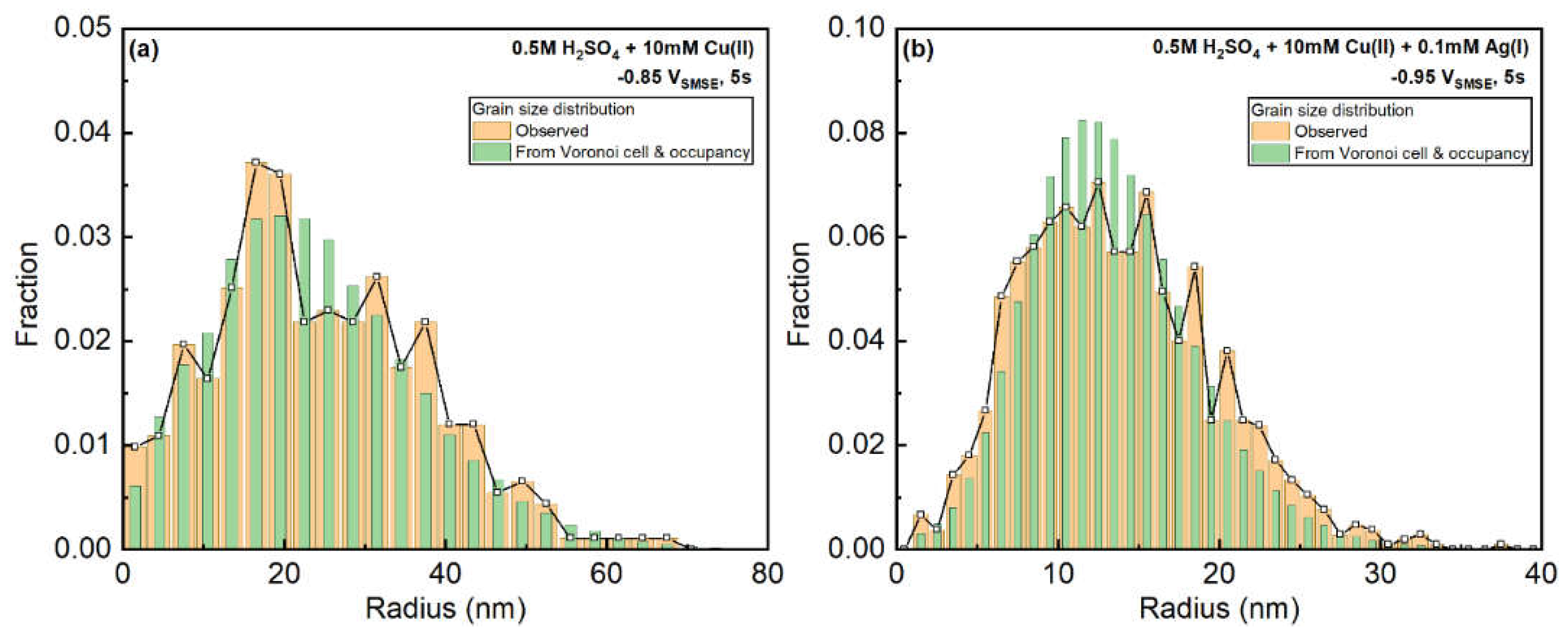
Since the Voronoi cell occupancy is defined with the area fraction of grains in each Voronoi cells, by assuming the partition of each Voronoi cell is independent of surrounding cells, we could derive the distribution of the grain size distribution from the distributions of Voronoi cell size and occupancy, by simply generating the histogram of each observed Voronoi cell size multipled by each Voronoi cell occupancy.
The observed and estimated grain size distribution are compared in Figure 13a,b. The Cu-only sample at -0.85VSMSE shows a good agreement between estimated and the observed distributions. However, the Ag-Cu sample at -0.95VSMSE reveals that the predicted distribution is narrower than the observed one. Such behavior suggests that larger Voronoi cells tends to have a larger occupation fraction and smaller cells have a smaller occupation. It is reasonable considering that the smaller nucleus are later formed and influenced by the diffusion fields from surrounding nuclei. Therefore, the diffusion fields from surrounding grains have less impact on the grain growth of Cu-only systems than Cu-Ag systems.
4.6. Spatial Distribution of Nuclei under Instantaneous and Progressive Nucleation Modes
In literature, the instantaneous nucleation mode was always simulated with spatially completely random points. However, features of the Cu-Ag deposits imply that nucleation exclusion behavior is more significant in the Cu-Ag systems than the Cu-only systems.
After examining the details in the classical model for the potentiostatic transients during electrodeposition, we found that following the assumptions on nucleation kinetics in S-H model (nucleation rate at the free area is proportional to the fraction of nucleation-exclusion-zone-free area), the instantaneous nucleation mode must be preceded by a progressive nucleation stage [70]. Following this statement, if the nucleation and growth in the electrodeposition system is only governed by the behavior of ions, the nuclei density for the instantaneous stage should also show an overpotential-dependence due to the progressive nucleation stage. Such behavior was not observed in our Cu-Ag deposits. Thus, the nucleation kinetics of the Cu-Ag samples (instantaneous mode) is not governed by the kinetics related to the Ag(I)/Ag deposition step. We hypothesize that the saturation nucleation density in those samples reflect the density of features (available nucleation sites) on the n-Si(001) substrate.
Regarding the spatial distribution of the nuclei, if the features at the substrate are completely spatially random, there will not be a progressive nucleation region in the potentiostatic transient, and the spatial distribution of nucleus will be spatially random. The spatial inhomogeneity observed in the Cu-Ag samples thus reflect the spatial inhomogenity of the available nucleation sites on the substrate.
5. Conclusion
In this work, we have examined the grain statistics and spatial distribution of Cu and Cu-Ag electrodeposits from acidic sulfate bath at fixed deposition cutoff time (5s) and different deposition potentials. The features of the grains could be fitted with Lognormal, Weibull or Gamma distributions. The grain size and Voronoi cell occupancy distributions could be better described by the Weibull distribution. The nearest neighbor distances, Voronoi cell size and grain coordination number could be better fitted with Gamma or Lognormal distributions. For reader’s reference, the fitting parameters were listed and compared.
Judging from SEM images, at given potential range and deposition cutoff time, the distribution of features of Cu-only systems depend strongly on the applied potential, whereas those of Cu-Ag are almost independent of the deposition potential. Thus, the Cu-only system is controlled by progressive nucleation of Cu whereas the Cu-Ag system is controlled by the instantaneous nucleation of Ag. At low deposition overpotential, Ag nucleus serves as reduction centers for Cu(II).
Surprisingly, the Cu-Ag system, seemingly to follow instantaneous nucleation kinetics, is more severely impact by the nucleation exclusion zones. By examining the details in the classical model for the potentiostatic transient, if the deposition is controlled by the reduction of ions (instead of substrate properties), all instantaneous nucleation modes should be preceded by a progressive nucleation stage. However, this behavior does not agree with the overpotential-independence of the nucleation densities in the Cu-Ag systems. Thus, the saturation nucleation density of Cu-Ag system is related to the nucleation site density of the substrate, and the distribution of Cu-Ag grains reflect the spatial inhomogeneity of those features on the substrate.
Acknowledgements
YKS thanks Wenbo Shao at MacDermid Alpha for kindly providing the SEM images used in this paper.
Credit author statement
Yunkai Sun: Conceptualization, Methodology, Writing - Original Draft, Writing - Review & Editing, Visualization; Giovanni Zangari: Conceptualization, Methodology, Resources, Project administration, Funding acquisition, Writing - Original Draft, Writing - Review & Editing.
References
- Scharifker, B.; Hills, G. Theoretical and experimental studies of multiple nucleation. Electrochimica Acta 1983, 28, 879–889. [Google Scholar] [CrossRef]
- Astley, D.; Harrison, J.; Thirsk, H. Electrocrystallization of mercury, silver and palladium. Trans. Faraday Soc. 1968, 64, 192–201. [Google Scholar] [CrossRef]
- Hyde, M.E.; Compton, R.G. A review of the analysis of multiple nucleation with diffusion controlled growth. Journal of Electroanalytical Chemistry 2003, 549, 1–12. [Google Scholar] [CrossRef]
- Barna, P.B.; Radnóczi, G. 3 - Structure formation during deposition of polycrystalline metallic thin films. In Metallic Films for Electronic, Optical and Magnetic Applications, Barmak, K., Coffey, K., Eds.; Woodhead Publishing: 2014; pp. 67-120.
- Ustarroz, J.; Hammons, J.A.; Altantzis, T.; Hubin, A.; Bals, S.; Terryn, H. A Generalized Electrochemical Aggregative Growth Mechanism. Journal of the American Chemical Society 2013, 135, 11550–11561. [Google Scholar] [CrossRef]
- Sun, Y.; Zangari, G. Grain statistics of electrodeposited Cu-Ag at n-Si(001) substrate, Part-1: Comparison of Gamma, Lognormal and Weibull distribution fits on the particle size distribution. Journal of The Electrochemical Society Submitted.
- Milchev, A.; Kruijt, W.S.; Sluyters-Rehbach, M.; Sluyters, J.H. Distribution of the nucleation rate in the vicinity of a growing spherical cluster: Part 1. Theory and simulation results. J. Electroanal. Chem. 1993, 362, 21–31. [Google Scholar] [CrossRef]
- Politi, S.; Tomellini, M. Kinetics of island growth in the framework of “planar diffusion zones” and “3D nucleation and growth” models for electrodeposition. Journal of Solid State Electrochemistry 2018, 22, 3085–3098. [Google Scholar] [CrossRef]
- Mostany, J.; Serruya, A.; Scharifker, B.R. Spatial distribution of electrodeposited lead nuclei on to vitreous carbon beyond their nearest neighbours. J. Electroanal. Chem. 1995, 383, 37–41. [Google Scholar] [CrossRef]
- Serruya, A.; Mostany, J.; Scharifker, B.R. Spatial distributions and saturation number densities of lead nuclei deposited on vitreous carbon electrodes. Journal of the Chemical Society, Faraday Transactions 1993, 89, 255–261. [Google Scholar] [CrossRef]
- Arzhanova, T.; Golikov, A. Long-range order in the spatial distribution of electrodeposited copper and silver nuclei on glassy carbon. Journal of Electroanalytical Chemistry 2003, 558, 109–117. [Google Scholar] [CrossRef]
- Arzhanova, T.; Golikov, A. Spatial distribution of copper nuclei electrodeposited on glassy carbon under galvanostatic conditions. Corrosion Science 2005, 47, 723–734. [Google Scholar] [CrossRef]
- Serruya, A.; Mostany, J.; Scharifker, B. The kinetics of mercury nucleation from Hg22+ and Hg2+ solutions on vitreous carbon electrodes. Journal of Electroanalytical Chemistry 1999, 464, 39–47. [Google Scholar] [CrossRef]
- Kruijt, W.S.; Sluyters-Rehbach, M.; Sluyters, J.H.; Milchev, A. Distribution of the nucleation rate in the vicinity of a growing spherical cluster.: Part 2. Theory of some special cases and experimental results. J. Electroanal. Chem. 1994, 371, 13–26. [Google Scholar] [CrossRef]
- Hyde, M.E.; Jacobs, R.M.; Compton, R.G. An electrodeposition study of the nucleation and growth of silver on boron-doped diamond electrodes. J. Electroanal. Chem. 2004, 562, 61–72. [Google Scholar] [CrossRef]
- Milchev, A.; Michailova, E.; Zapryanova, T. Initial stages of electrochemical alloy formation: size and composition of critical nuclei. Electrochemistry Communications 2004, 6, 713–718. [Google Scholar] [CrossRef]
- Moehl, G.E.; Bartlett, P.N.; Hector, A.L. Using GISAXS to Detect Correlations between the Locations of Gold Particles Electrodeposited from an Aqueous Solution. Langmuir 2020, 36, 4432–4438. [Google Scholar] [CrossRef]
- Scharifker, B.R.; Mostany, J.; Serruya, A. On the spatial distribution of nuclei on electrode surfaces. Electrochim. Acta 1992, 37, 2503–2510. [Google Scholar] [CrossRef]
- Tsakova, V.; Milchev, A. Spatial distribution of electrochemically deposited clusters: a simulation study1Dedicated to acad. R. Kaischer on the occasion of his 90th birthday.1. J. Electroanal. Chem. 1998, 451, 211–218. [Google Scholar] [CrossRef]
- Torquato, S.; Lu, B.; Rubinstein, J. Nearest-neighbor distribution functions in many-body systems. Phys. Rev. A 1990, 41, 2059. [Google Scholar] [CrossRef]
- Tomellini, M. Spatial distribution of nuclei in progressive nucleation: Modeling and application. Physica A: Statistical Mechanics and its Applications 2018, 496, 481–494. [Google Scholar] [CrossRef]
- Tomellini, M. Interface evolution in phase transformations ruled by nucleation and growth. Physica A: Statistical Mechanics and its Applications 2020, 558, 124981. [Google Scholar] [CrossRef]
- Barmak, K.; Eggeling, E.; Kinderlehrer, D.; Sharp, R.; Ta’asan, S.; Rollett, A.D.; Coffey, K.R. Grain growth and the puzzle of its stagnation in thin films: The curious tale of a tail and an ear. Progress in Materials Science 2013, 58, 987–1055. [Google Scholar] [CrossRef]
- Shao, W.; Sun, Y.; Zangari, G. Electrodeposition of Cu-Ag Alloy Films at n-Si(001) and Polycrystalline Ru Substrates. Coatings 2021, 11, 1563. [Google Scholar] [CrossRef]
- Shao, W.; Sun, Y.; Giurlani, W.; Innocenti, M.; Zangari, G. Estimating electrodeposition properties and processes: Cu-Ag alloy at n-Si(001) and Ru substrates from acidic sulfate bath. Electrochimica Acta 2022, 403, 139695. [Google Scholar] [CrossRef]
- Shao, W. Electrochemical Nucleation and Growth of Copper and Copper Alloys. 2008, Charlottesville, VA, 2008.
- Bayat, H.; Rastgo, M.; Mansouri Zadeh, M.; Vereecken, H. Particle size distribution models, their characteristics and fitting capability. Journal of Hydrology 2015, 529, 872–889. [Google Scholar] [CrossRef]
- Haenggi, M. On distances in uniformly random networks. IEEE Transactions on Information Theory 2005, 51, 3584–3586. [Google Scholar] [CrossRef]
- Tong, W.; Rickman, J.; Barmak, K. Impact of short-range repulsive interactions between nuclei on the evolution of a phase transformation. J. Chem. Phys. 2001, 114, 915–922. [Google Scholar] [CrossRef]
- Noufaily, A.; Jones, M.C. Parametric quantile regression based on the generalized gamma distribution. Journal of the Royal Statistical Society: Series C (Applied Statistics) 2013, 62, 723–740. [Google Scholar] [CrossRef]
- Song, K. Globally Convergent Algorithms for Estimating Generalized Gamma Distributions in Fast Signal and Image Processing. IEEE Transactions on Image Processing 2008, 17, 1233–1250. [Google Scholar] [CrossRef]
- Shang, X.; Ng, H.K.T. On parameter estimation for the generalized gamma distribution based on left-truncated and right-censored data. Computational and Mathematical Methods n/a e1091. [CrossRef]
- Lienhard, J.H.; Meyer, P.L. A physical basis for the generalized gamma distribution. Quarterly of Applied Mathematics 1967, 25, 330–334. [Google Scholar] [CrossRef]
- Rinne, H. The Weibull distribution: a handbook; CRC Press: Boca Raton, 2009. [Google Scholar]
- Rinne, H. 1.2 Physical meanings and interpretations of the Weibull distribution. In The Weibull distribution : a handbook; CRC Press: Boca Raton, 2009; pp. 15–26. [Google Scholar]
- Louat, N.P. On the theory of normal grain growth. Acta Metallurgica 1974, 22, 721–724. [Google Scholar] [CrossRef]
- Fayad, W.; Thompson, C.V.; Frost, H.J. Steady-state grain-size distributions resulting from grain growth in two dimensions. Scripta Materialia 1999, 40, 1199–1204. [Google Scholar] [CrossRef]
- Stauffer, H. A derivation for the Weibull distribution. Journal of theoretical biology 1979, 81, 55–63. [Google Scholar] [CrossRef] [PubMed]
- Limpert, E.; Stahel, W.A.; Abbt, M. Log-normal Distributions across the Sciences: Keys and Clues: On the charms of statistics, and how mechanical models resembling gambling machines offer a link to a handy way to characterize log-normal distributions, which can provide deeper insight into variability and probability—normal or log-normal: That is the question. BioScience 2001, 51, 341–352. [Google Scholar] [CrossRef]
- Mitzenmacher, M. A Brief History of Generative Models for Power Law and Lognormal Distributions. Draft manuscript.
- Brown, G.; Sanders, J. Lognormal genesis. Journal of Applied probability 1981, 542–547. [Google Scholar] [CrossRef]
- Brown, G.; Sanders, J.W. Lognormal Genesis. Journal of Applied Probability 1981, 18, 542–547. [Google Scholar] [CrossRef]
- Parkin, T.; Robinson, J. Analysis of lognormal data. In Advances in soil science; Springer: 1992; pp. 193-235.
- Lognormal Distribution. The Concise Encyclopedia of Statistics; Springer New York: New York, NY, 2008; pp. 321–322. [Google Scholar]
- Aitchison, J.; Brown, J.A.C. The Lognormal Distribution: With Special Reference to Its Uses in Economics; University Press: 1966.
- Loper, J.; Suslow, T.; Schroth, M. Lognormal distribution of bacterial populations in the rhizosphere. Phytopathology 1984, 74, 1454–1460. [Google Scholar] [CrossRef]
- Rohrer, G.S.; Liu, X.; Liu, J.; Darbal, A.; Kelly, M.N.; Chen, X.; Berkson, M.A.; Nuhfer, N.T.; Coffey, K.R.; Barmak, K. The grain boundary character distribution of highly twinned nanocrystalline thin film aluminum compared to bulk microcrystalline aluminum. Journal of Materials Science 2017, 52, 9819–9833. [Google Scholar] [CrossRef]
- Thomas, J.C. The determination of log normal particle size distributions by dynamic light scattering. Journal of Colloid and Interface Science 1987, 117, 187–192. [Google Scholar] [CrossRef]
- López, R.E. The Lognormal Distribution and Cumulus Cloud Populations. Monthly Weather Review 1977, 105, 865–872. [Google Scholar] [CrossRef]
- Kosugi, K.i. Lognormal Distribution Model for Unsaturated Soil Hydraulic Properties. Water Resources Research 1996, 32, 2697–2703. [Google Scholar] [CrossRef]
- Akhundjanov, S.B.; Toda, A.A. Is Gibrat’s “Economic Inequality” lognormal? Empirical Economics 2019. [Google Scholar] [CrossRef]
- Karasev, B. Statistical genesis of a lognormal distribution as a source of properties observed in the clumping of galaxies. Soviet Astronomy Letters 1982, 8, 284–287. [Google Scholar]
- Royston, P. The lognormal distribution as a model for survival time in cancer, with an emphasis on prognostic factors. Statistica Neerlandica 2001, 55, 89–104. [Google Scholar] [CrossRef]
- Sheridan, P.; Onodera, T. A Preferential Attachment Paradox: How Preferential Attachment Combines with Growth to Produce Networks with Log-normal In-degree Distributions. Scientific Reports 2018, 8, 2811. [Google Scholar] [CrossRef]
- Strum, D.P.; May, J.H.; Vargas, L.G. Modeling the uncertainty of surgical procedure times: comparison of log-normal and normal models. Anesthesiology 2000, 92, 1160–1167. [Google Scholar] [CrossRef]
- Sobkowicz, P.; Thelwall, M.; Buckley, K.; Paltoglou, G.; Sobkowicz, A. Lognormal distributions of user post lengths in Internet discussions - a consequence of the Weber-Fechner law? EPJ Data Science 2013, 2, 2. [Google Scholar] [CrossRef]
- Kolmogoroff, A. Über das logarithmisch normale Verteilungsgesetz der Dimensionen der Teilchen bei Zerstückelung. In Proceedings of the CR (Doklady) Acad. Sci. URSS (NS); 1941; pp. 99–101. [Google Scholar]
- Kolmogorov, A. On the Logarithmic Normal Distribution of Particle Sizes under Grinding. In Selected works of AN Kolmogorov: Volume II probability theory and mathematical statistics, Shiryayev, A.N., Ed.; Springer Science & Business Media:,1992; Volume 26, pp. 281-284.
- Gorokhovski, M.A.; Saveliev, V.L. Analyses of Kolmogorov’s model of breakup and its application into Lagrangian computation of liquid sprays under air-blast atomization. Physics of Fluids 2003, 15, 184–192. [Google Scholar] [CrossRef]
- Bergmann, R.B.; Bill, A. On the origin of logarithmic-normal distributions: An analytical derivation, and its application to nucleation and growth processes. Journal of Crystal Growth 2008, 310, 3135–3138. [Google Scholar] [CrossRef]
- Teran, A.V.; Bill, A.; Bergmann, R.B. Time-evolution of grain size distributions in random nucleation and growth crystallization processes. Physical Review B 2010, 81, 075319. [Google Scholar] [CrossRef]
- Gunawardena, G.; Hills, G.; Montenegro, I.; Scharifker, B. Electrochemical nucleation: Part I. General considerations. J. Electroanal. Chem. 1982, 138, 225–239. [Google Scholar] [CrossRef]
- Goh, S.; Kwon, H.W.; Choi, M.Y.; Fortin, J.Y. Emergence of skew distributions in controlled growth processes. Phys. Rev. E 2010, 82, 061115. [Google Scholar] [CrossRef]
- Ming Tan, C.; Raghavan, N.; Roy, A. Application of gamma distribution in electromigration for submicron interconnects. J. Appl. Phys. 2007, 102, 103703. [Google Scholar] [CrossRef]
- Walck, C. 17 Gamma Distribution. In Hand-book on statistical distributions for experimentalists; University of Stockholm, 2007; pp. 69-72.
- Pineda, E.; Garrido, V.; Crespo, D. Domain-size distribution in a Poisson-Voronoi nucleation and growth transformation. Phys. Rev. E 2007, 75, 040107. [Google Scholar] [CrossRef] [PubMed]
- Ferenc, J.-S.; Néda, Z. On the size distribution of Poisson Voronoi cells. Physica A: Statistical Mechanics and its Applications 2007, 385, 518–526. [Google Scholar] [CrossRef]
- Tong, W.; Rickman, J.M.; Barmak, K. Impact of boundary nucleation on product grain size distribution. Journal of materials research 1997, 12, 1501–1507. [Google Scholar] [CrossRef]
- Tong, W.; Rickman, J.; Barmak, K. Quantitative analysis of spatial distribution of nucleation sites: microstructural implications. Acta materialia 1999, 47, 435–445. [Google Scholar] [CrossRef]
- Sun, Y.; Zangari, G. Grain statistics of electrodeposited Cu-Ag at n-Si(001) substrate, Part-3: Commentary and notes on the original derivations of the Scharifker-Hills model In preparation.
Figure 1.
SEM images of the Cu-only and Cu-Ag samples used in this work. Deposition stops at 5s for all samples. The red lines indicate the boundary of the identified grains after image processing. 0.5M H2SO4 was used as the supporting electrolyte. All the other deposition parameters are listed in the figures. Original SEM images are included in Appendix A.
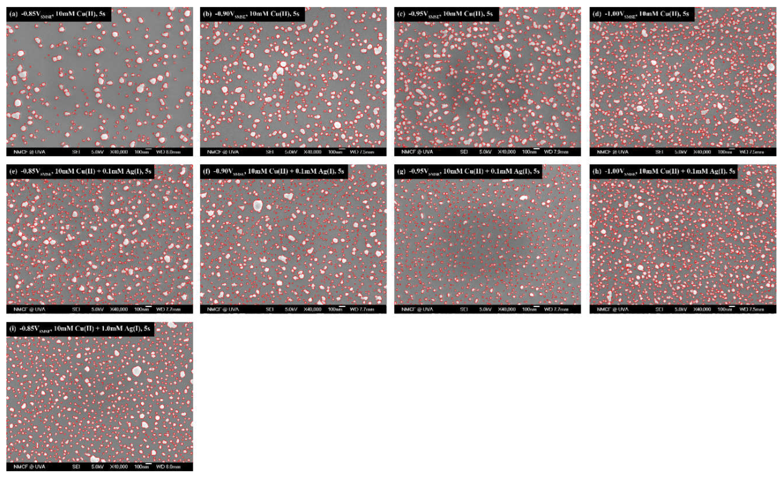
Figure 2.
Comparison between Gamma fitting results from different definitions of grain sizes and Lognormal or Weibull fitting results.
Figure 2.
Comparison between Gamma fitting results from different definitions of grain sizes and Lognormal or Weibull fitting results.
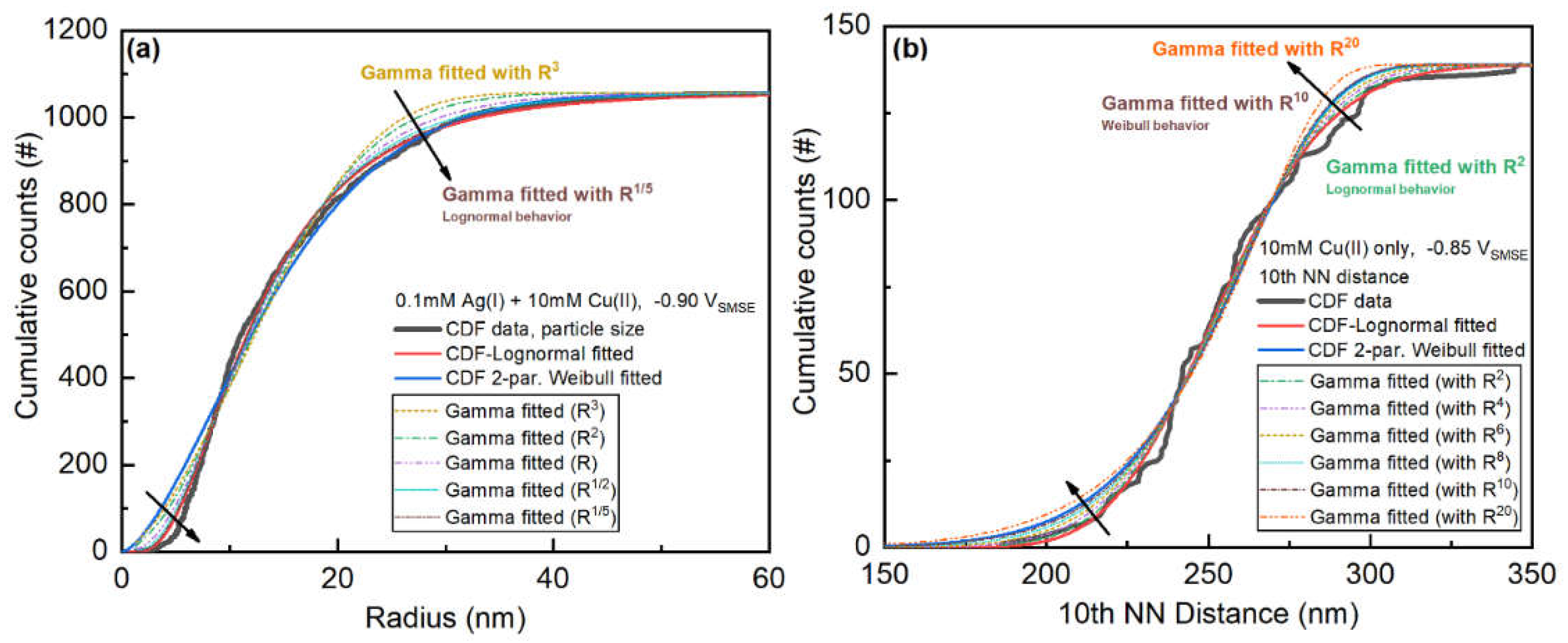
Figure 3.
summary of the statistics of the SEM images: (a,b,c) mean radius/length, (d,e,f) standard deviation, and (g,h,i) skewness. Note that the occupancy is based on area fraction of the grains inside their Voronoi cells. The mean, standard deviation, and skewness of the grain and Voronoi cell sizes are evaluated based on their linear size assuming the particles are circular (). Values in this figure are tabulated in Appendix D.
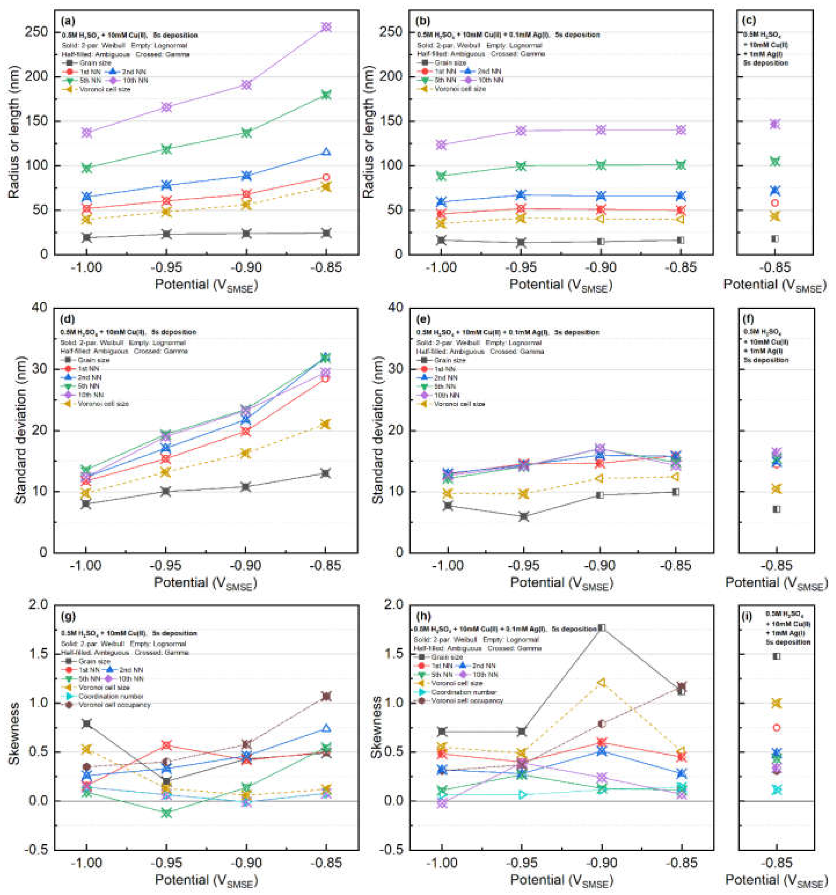
Figure 4.
Fitting results of the features with Weibull distribution in parameter (a,b,c) and Lognormal distribution in parameter (d,e,f). Location of was marked in the Weibull distribution figures (a,b,c), which value corresponds to the grain size statistics in a 2D steady state grain growth simulation by Fayad et al. [37].
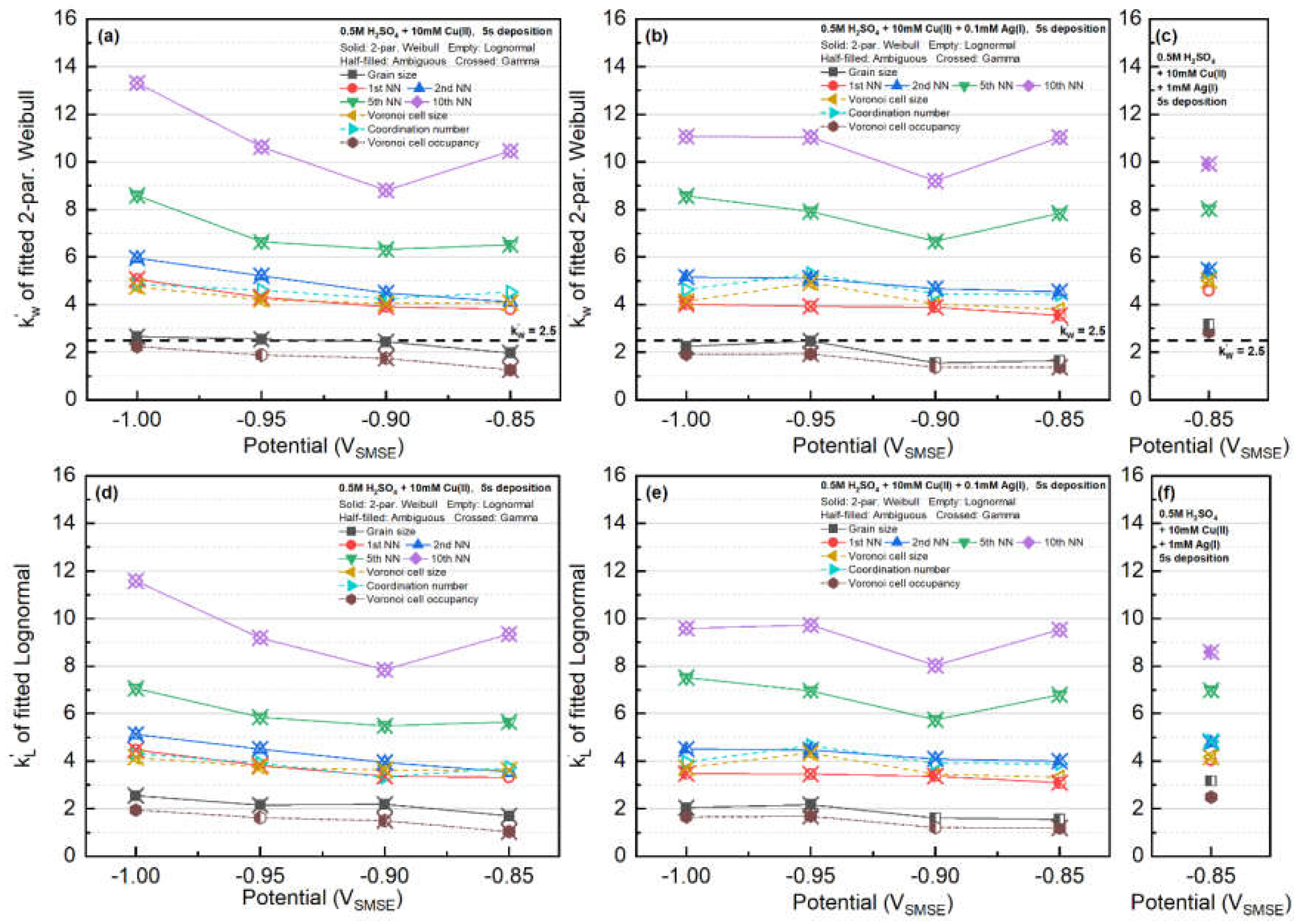
Figure 5.
Fitting results of the Gamma distribution with both fitting parameters.
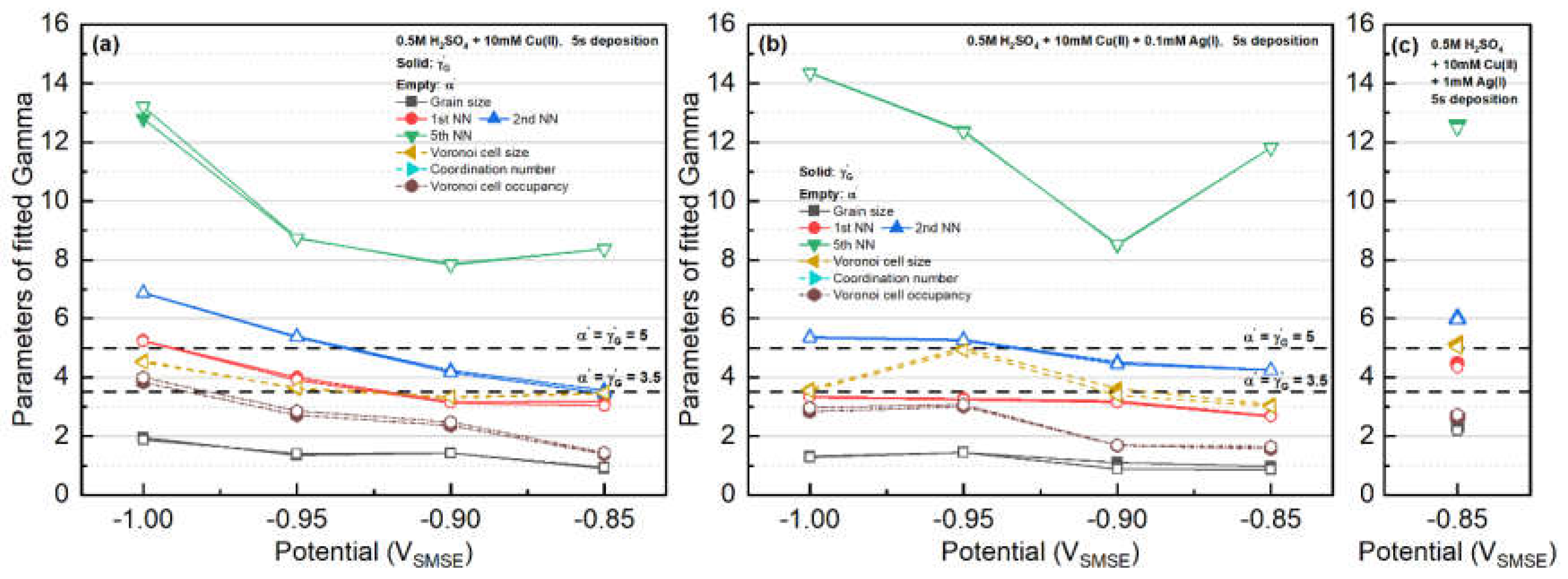
Figure 6.
Particle size distributions for all the Cu-only and Cu-Ag samples.
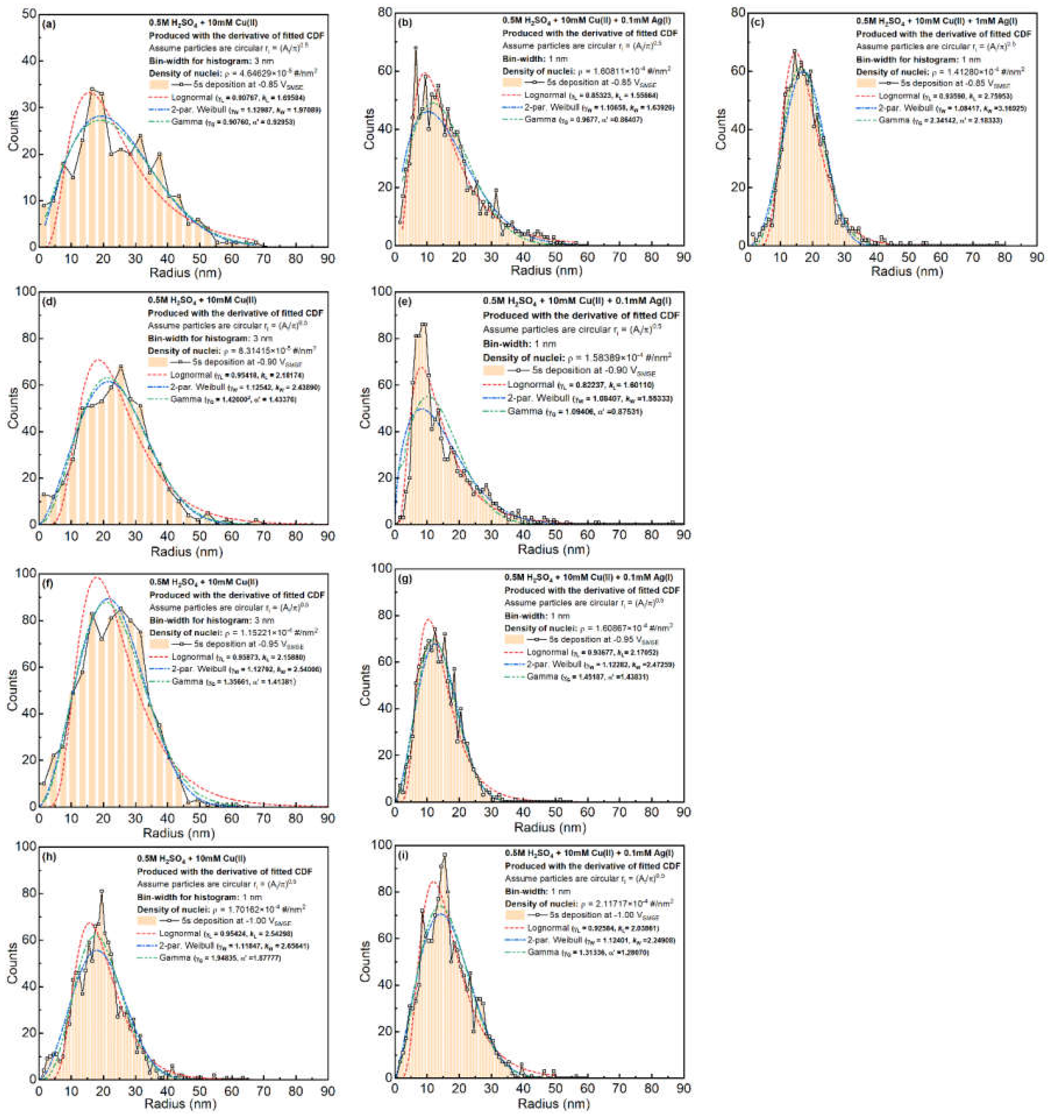
Figure 7.
Voronoi cell size distributions for all Cu-only and Cu-Ag samples. Average radius is calculated based on average area assuming circular shape (instead of the average of the linear dimensions of the Voronoi cells).
Figure 7.
Voronoi cell size distributions for all Cu-only and Cu-Ag samples. Average radius is calculated based on average area assuming circular shape (instead of the average of the linear dimensions of the Voronoi cells).
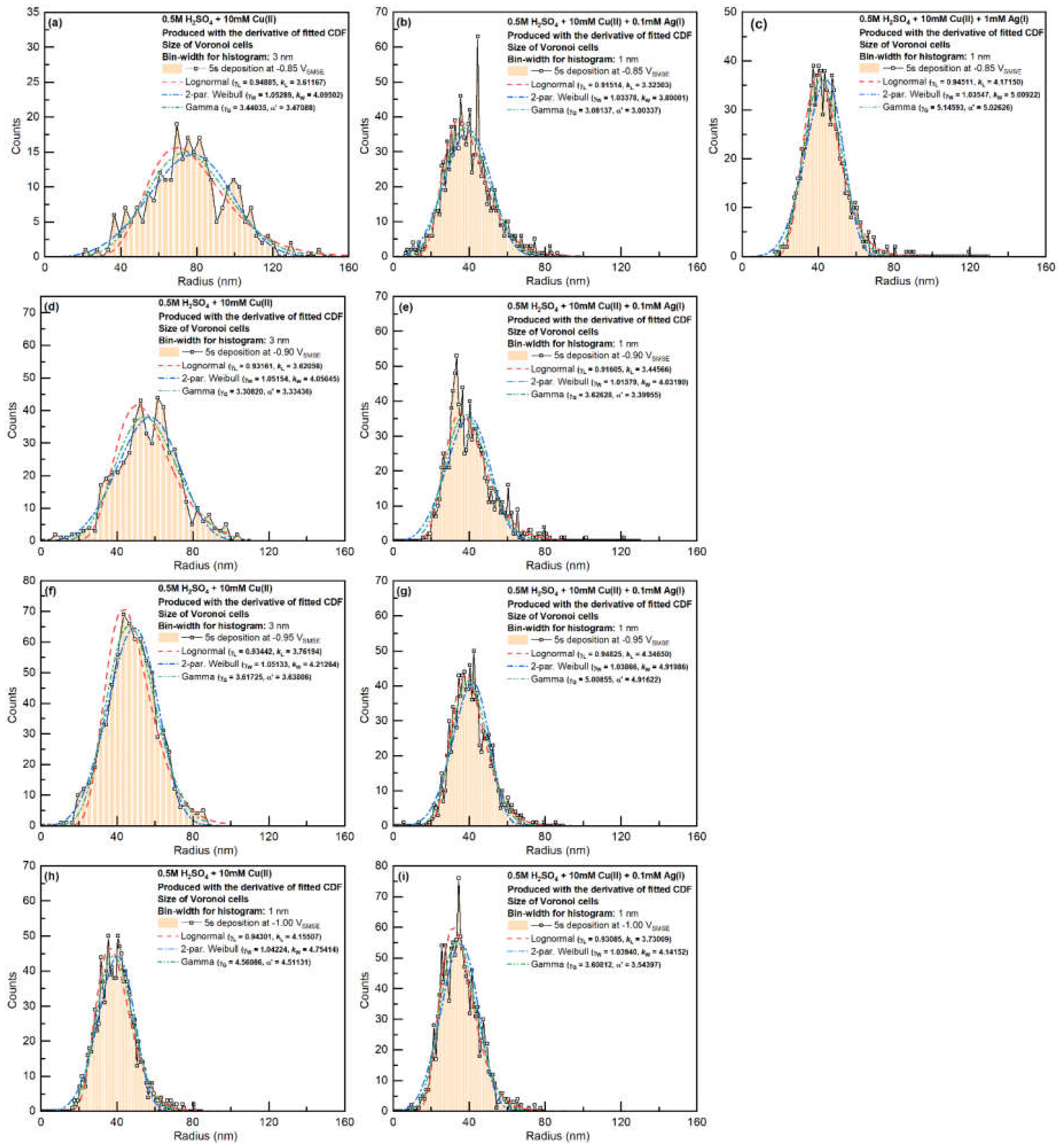
Figure 8.
Voronoi cell area occupancy.

Figure 9.
NN distance distribution for 10mM Cu(II) at different deposition potentials. Image size: 3000 2250 nm2.
Figure 9.
NN distance distribution for 10mM Cu(II) at different deposition potentials. Image size: 3000 2250 nm2.
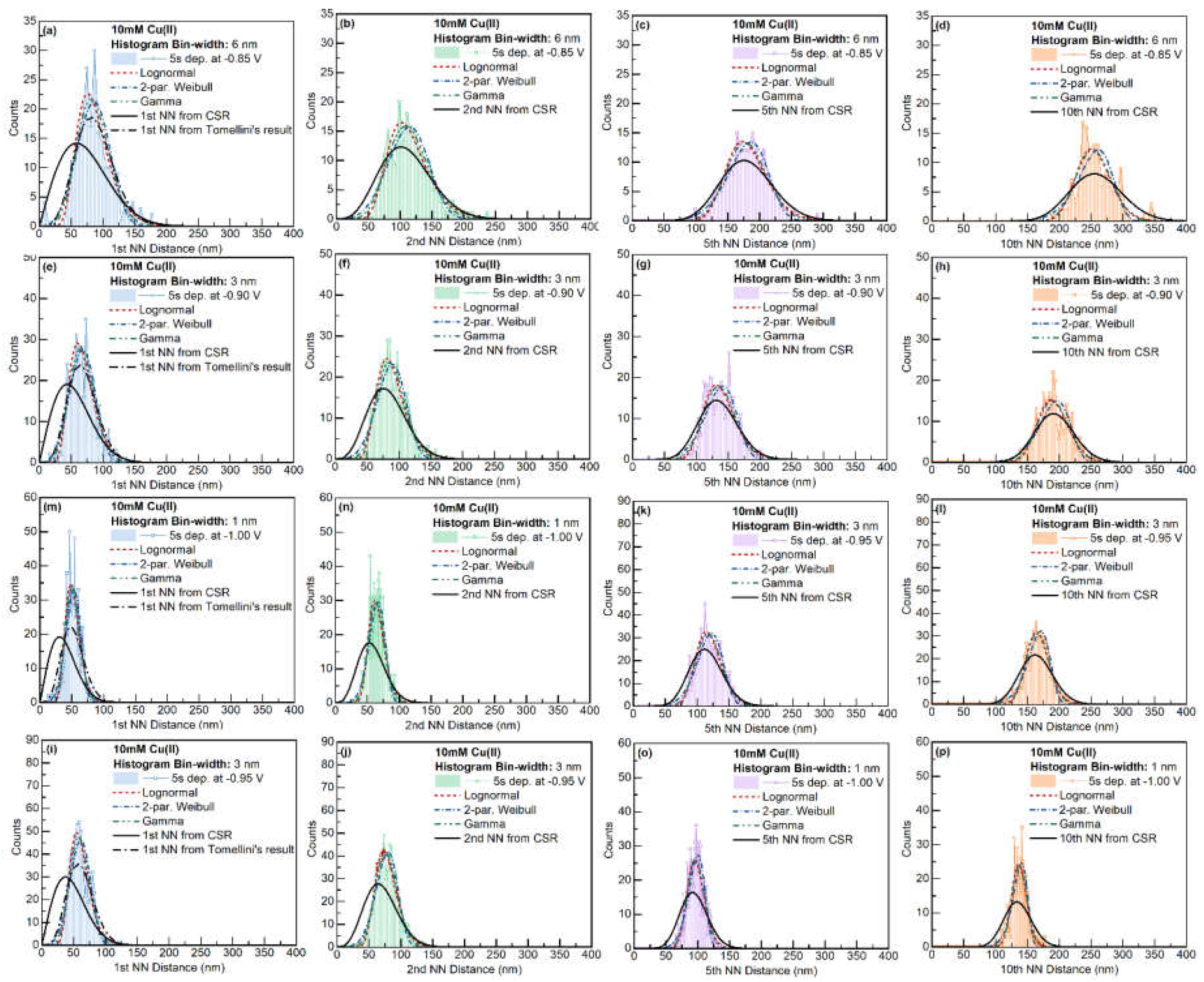
Figure 10.
NN distance distribution for 10mM Cu(II) + 0.1 or 1mM Ag(I) at different deposition potentials. Image size: 3000 2250 nm2.
Figure 10.
NN distance distribution for 10mM Cu(II) + 0.1 or 1mM Ag(I) at different deposition potentials. Image size: 3000 2250 nm2.
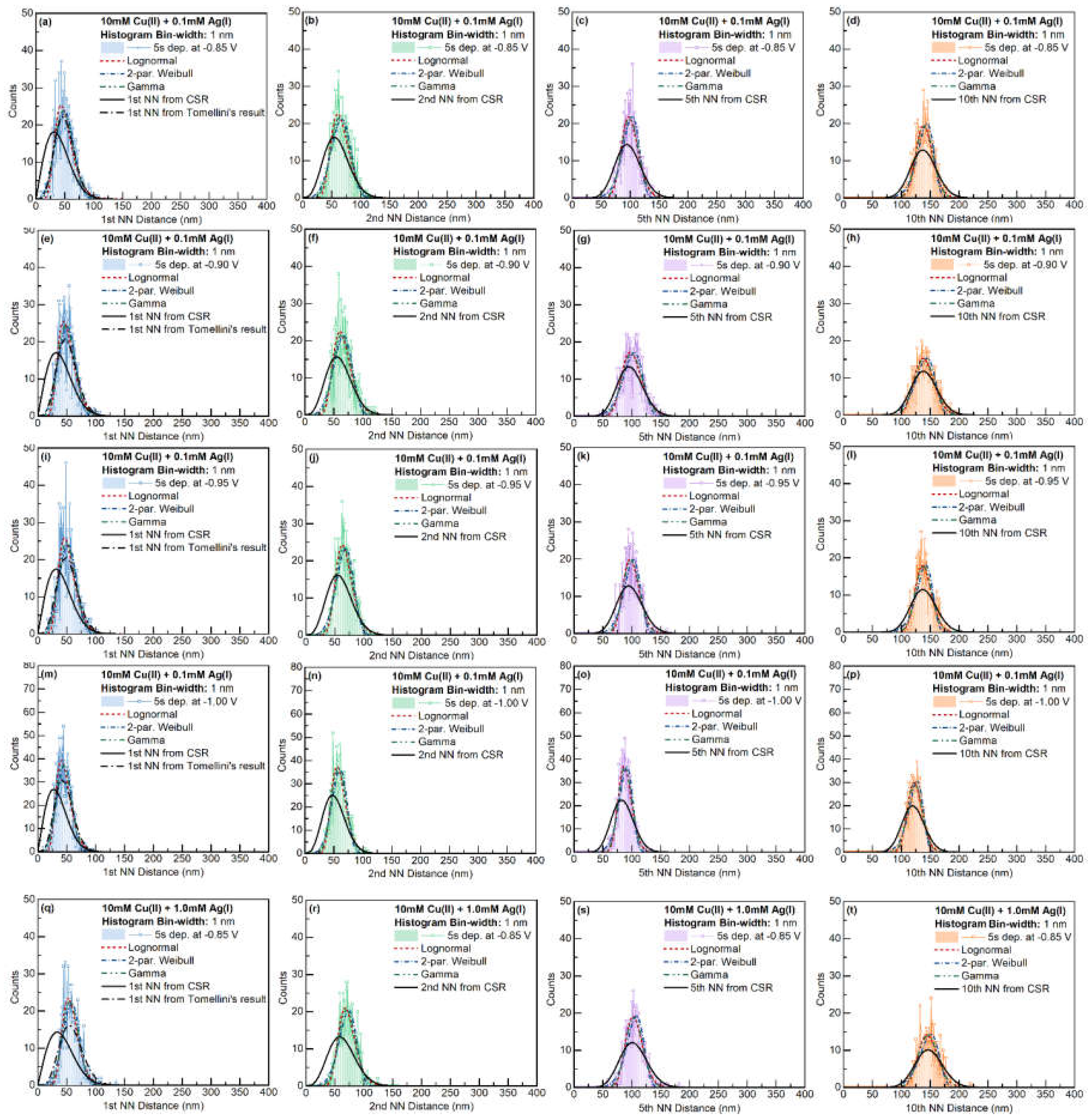
Figure 11.
(a) Log-log plot of the mean distance of the pair of nuclei neighbor and (b) standard deviations of the 1-12 ranks of nearest neighbor distances. Both values are normalized based on the nucleation density (instead of average distance). Values corresponding to the nearest neighbor distance of spatially completely random points are drawn as reference lines.
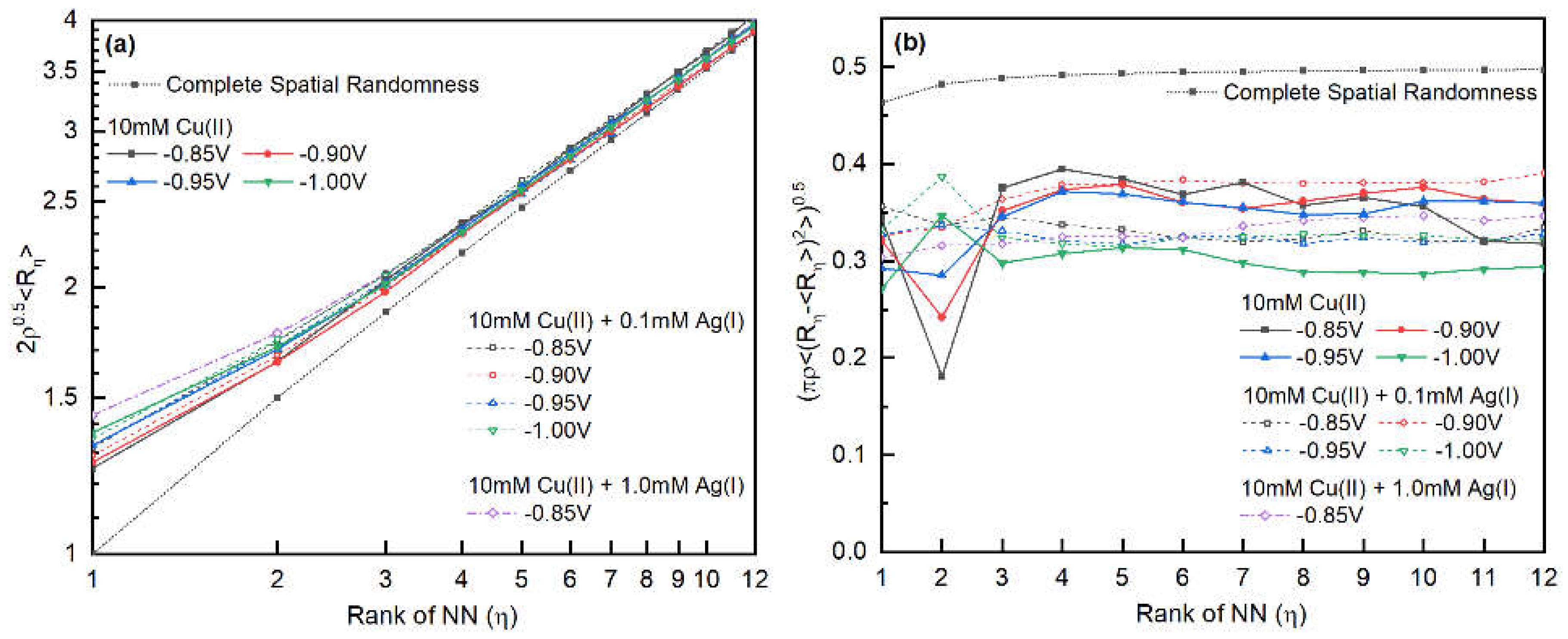
Figure 12.
RDF of the (a) Cu-only samples and (b) Cu-Ag samples at various deposition potentials. Vertical dotted lines are the average diameter of the grains. The horizontal dashed line is the radial distribution function with complete spatial randomness.
Figure 12.
RDF of the (a) Cu-only samples and (b) Cu-Ag samples at various deposition potentials. Vertical dotted lines are the average diameter of the grains. The horizontal dashed line is the radial distribution function with complete spatial randomness.
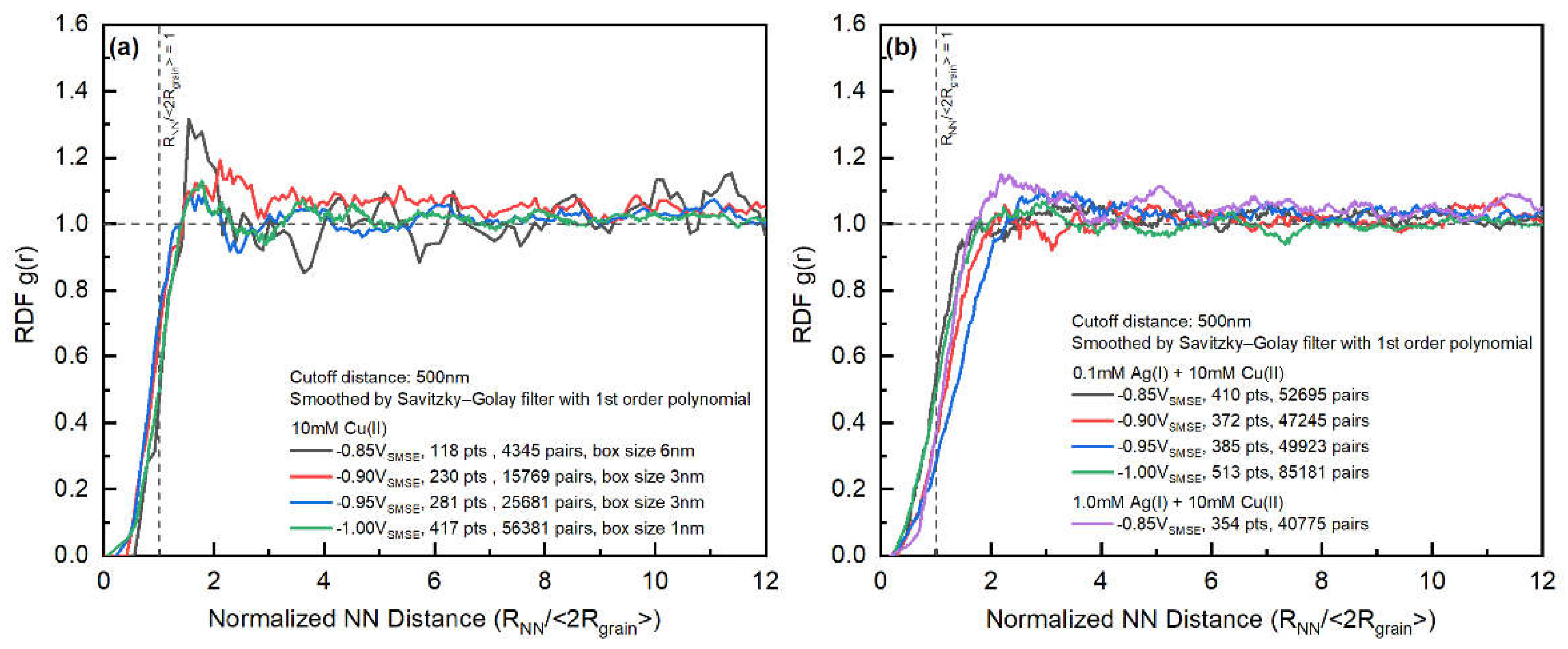
Figure 13.
Comparison between observed and estimated (from Voronoi cell size and occupancy) grain sizes. (a) Cu-only deposits from 10mM Cu(II) electrolyte at -0.85VSMSE for 5 seconds. (b) Cu-Ag deposits from 10mM Cu(II) + 0.1mM Ag(I) electrolyte at -0.95VSMSE for 5 seconds.
Figure 13.
Comparison between observed and estimated (from Voronoi cell size and occupancy) grain sizes. (a) Cu-only deposits from 10mM Cu(II) electrolyte at -0.85VSMSE for 5 seconds. (b) Cu-Ag deposits from 10mM Cu(II) + 0.1mM Ag(I) electrolyte at -0.95VSMSE for 5 seconds.
Disclaimer/Publisher’s Note: The statements, opinions and data contained in all publications are solely those of the individual author(s) and contributor(s) and not of MDPI and/or the editor(s). MDPI and/or the editor(s) disclaim responsibility for any injury to people or property resulting from any ideas, methods, instructions or products referred to in the content. |
© 2023 by the authors. Licensee MDPI, Basel, Switzerland. This article is an open access article distributed under the terms and conditions of the Creative Commons Attribution (CC BY) license (http://creativecommons.org/licenses/by/4.0/).
Copyright: This open access article is published under a Creative Commons CC BY 4.0 license, which permit the free download, distribution, and reuse, provided that the author and preprint are cited in any reuse.


