Submitted:
22 August 2023
Posted:
23 August 2023
You are already at the latest version
Abstract
Keywords:
1. Introduction
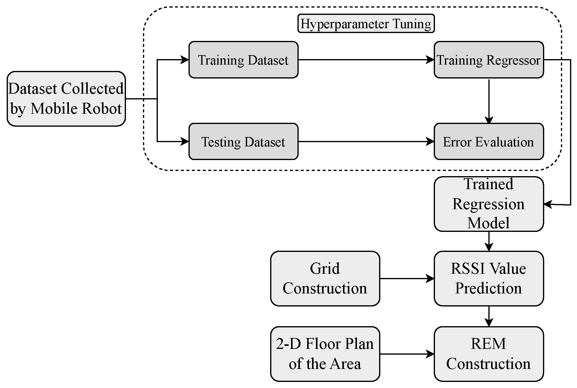
- We propose an ML-based approach to obtain the indoor coverage map and accurately localize users by harnessing the potential of RSSI signals.
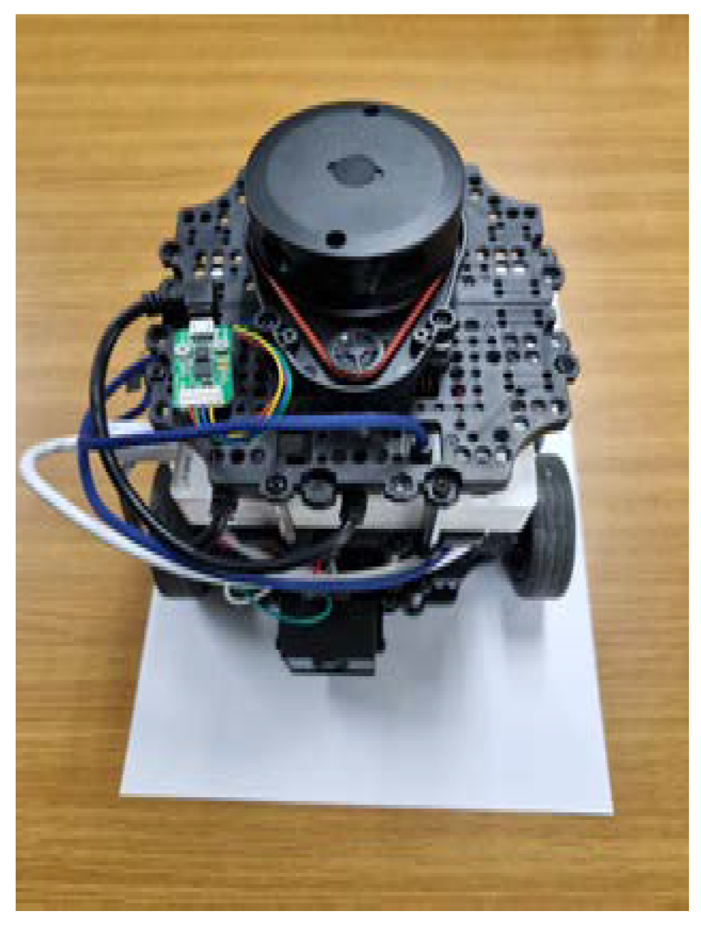
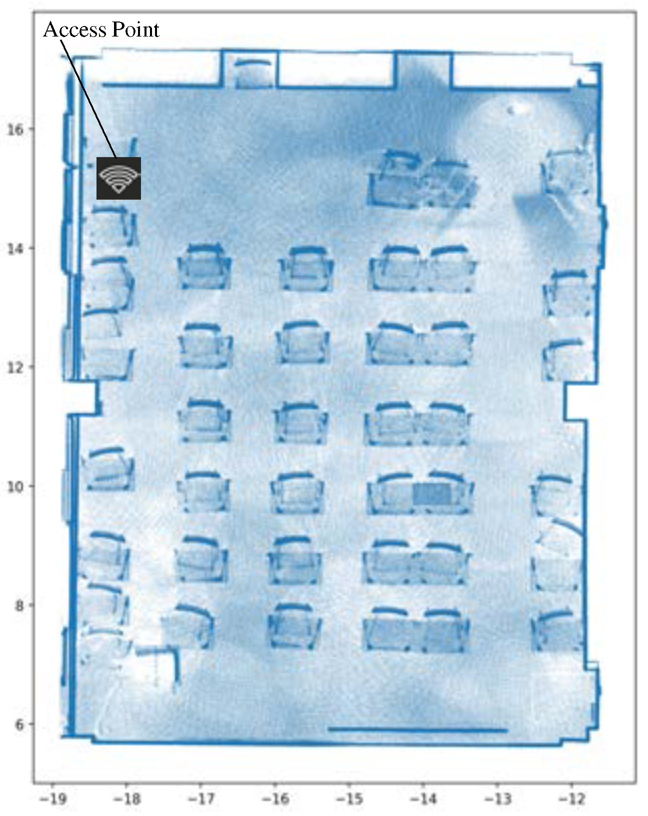
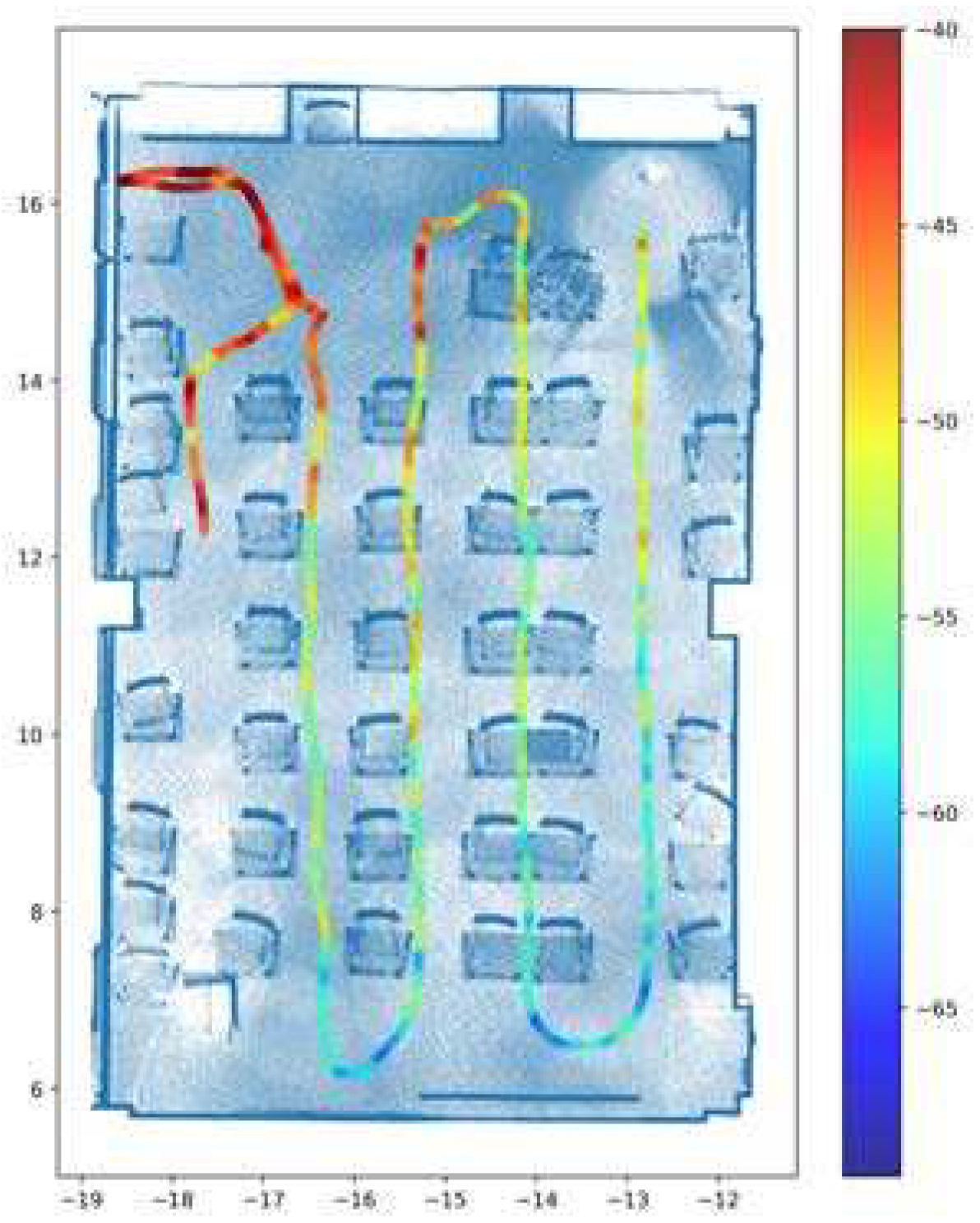
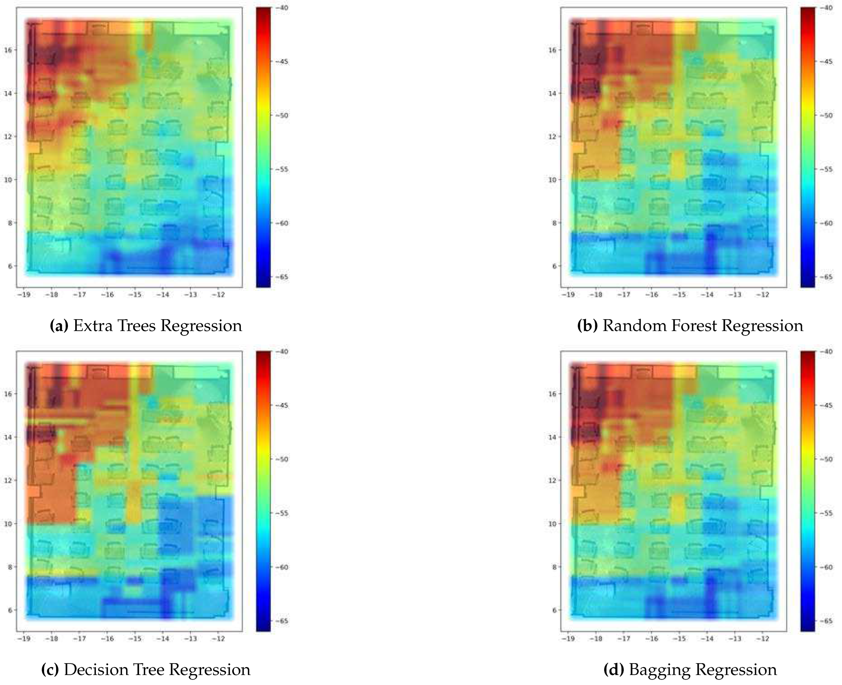
- Construction of the REM is based on an ML scheme using a single AP to collect RSSI measurements from a mobile robot. This strategic approach enables operators to gain clear visibility into coverage prediction and identify potential shadow areas on the indoor REM. In our study, we focus on localization by leveraging a coverage prediction map specifically considering RSSI signals within an indoor environment of the University of Ulsan.
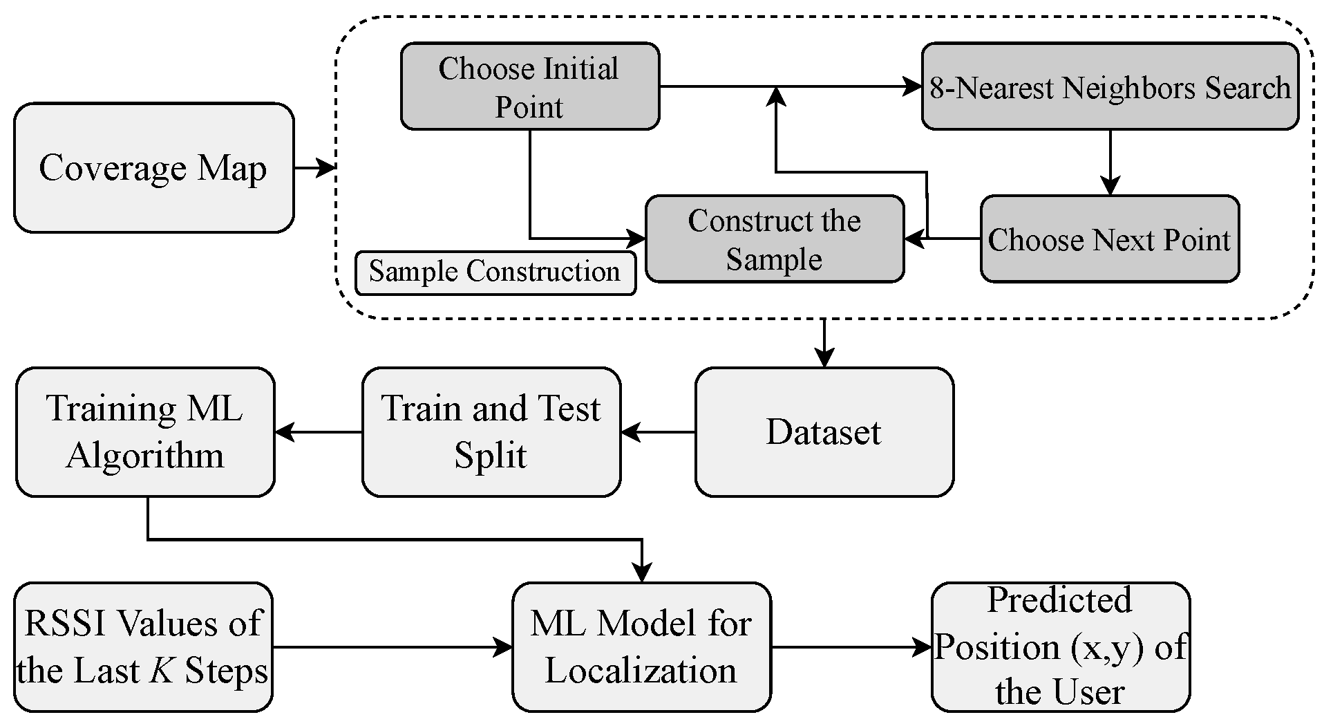
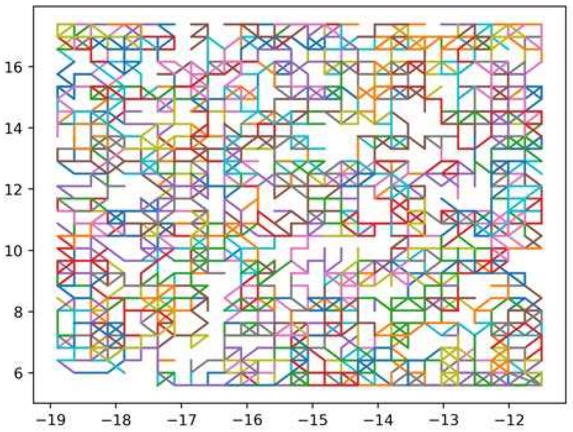
- To construct the dataset used to train our ML algorithm for localization, the selection of each step is primarily based on a nearest neighbors search. Within each sample, we choose the first point randomly and then obtain eight nearest neighbors to determine the next step. This iterative process continues for K steps. By diligently following this procedure, we construct a single sample. This process is repeated until we reach the defined number of samples for the dataset.
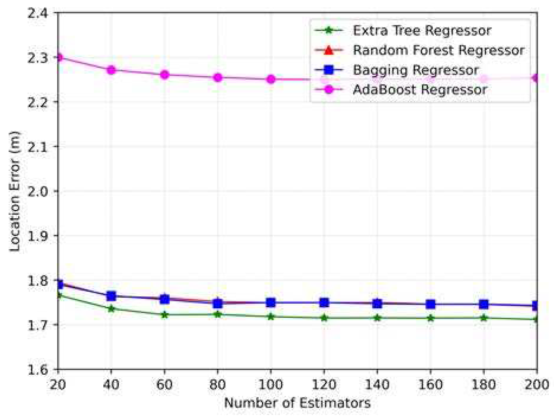
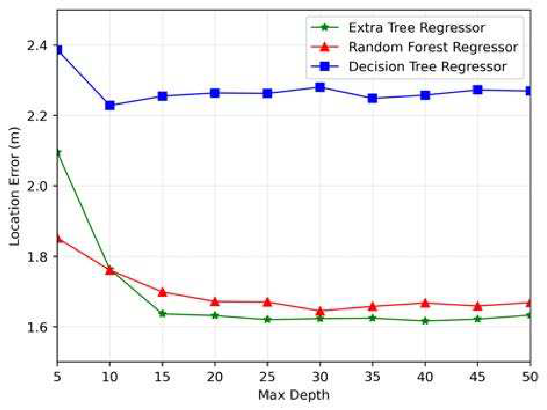
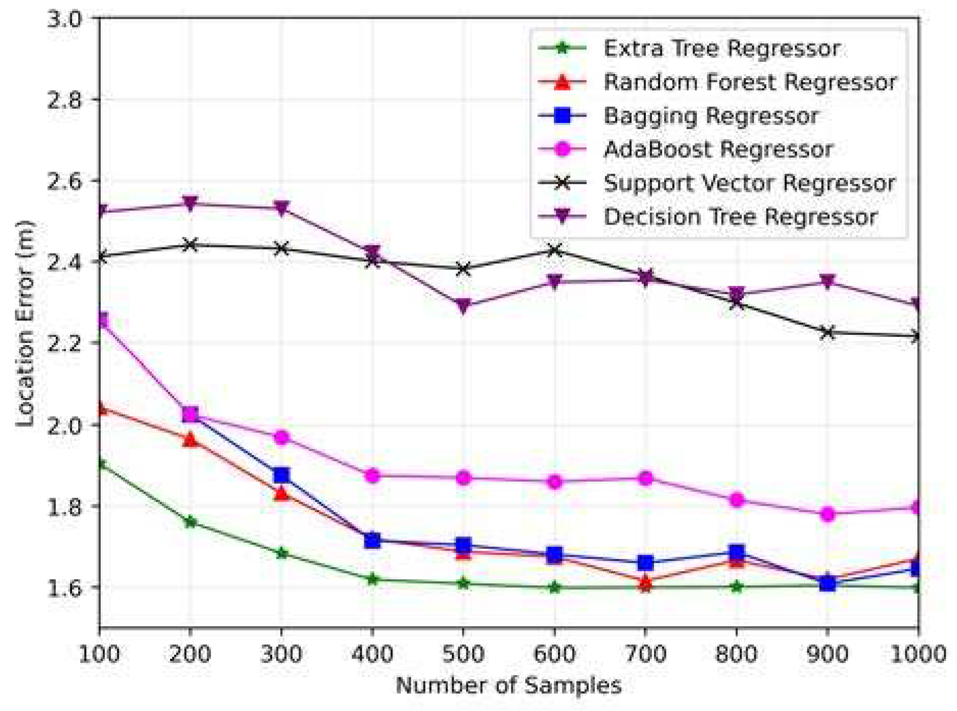
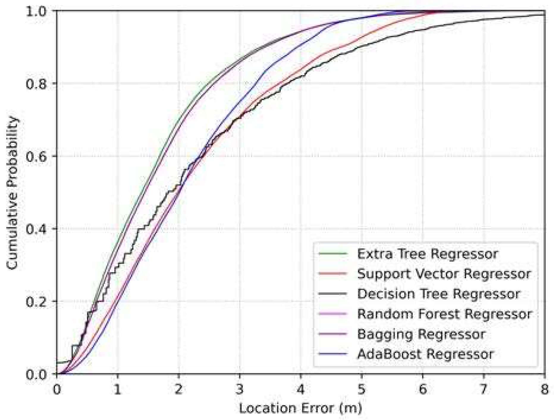
- We meticulously analyzed several prominent ML algorithms, namely the random forest regression [21], decision tree regression [22], extra trees regression (ETR) [20], and adaBoost regression [23], etc. Through the rigorous application of the 10-fold cross-validation technique, we aim to identify the optimal regressor algorithm for our proposed approach by considering the localization error.
2. Related Work
3. Measurement Methodology
4. Proposed Methodology
4.1. General Overview
4.2. Dataset Construction
4.3. ETR Framework for Indoor Localization
5. Machine Learning Regression Baseline Schemes
5.1. Random Forest Regressor
5.2. AdaBoost Regressor
5.3. Decision Tree Regressor
6. Numerical Results
6.1. Model Evaluation
| Algorithm | RMSE | MAE | |
|---|---|---|---|
| Extra Trees Regression | 0.997 | 0.975 | 0.421 |
| Random Forest Regression | 1.067 | 0.971 | 0.49 |
| Decision Tree Regression | 1.218 | 0.963 | 0.47 |
| Bagging Regression | 1.064 | 0.972 | 0.492 |
| Support Vector Regression | 2.977 | 0.779 | 2.317 |
| AdaBoost Regression | 2.874 | 0.794 | 2.301 |
6.2. Computational Complexity Analysis
6.3. Graphical Results of REM Construction
7. Conclusion
References
- Zhang, K.; Zhao, J.; Liu, P.; Yin, C. Radio Environment Map Enhanced Intelligent Reflecting Surface Systems Beyond 5G. In Proceedings of the 2021 IEEE International Conference on Communications Workshops (ICC Workshops). IEEE; 2021; pp. 1–6. [Google Scholar]
- McGuire, M.; Plataniotis, K.N.; Venetsanopoulos, A.N. Data fusion of power and time measurements for mobile terminal location. IEEE Transactions on Mobile Computing 2005, 4, 142–153. [Google Scholar] [CrossRef]
- Sytems, C. Wi-Fi based real-time location tracking: Solutions and technology. In CISCO Syt.; 2006.
- Patterson, C.A.; Muntz, R.R.; Pancake, C.M. Challenges in location-aware computing. IEEE Pervasive Computing 2003, 2, 80–89. [Google Scholar] [CrossRef]
- Rodríguez, M.D.; Favela, J.; Martínez, E.A.; Muñoz, M.A. Location-aware access to hospital information and services. IEEE Transactions on information technology in biomedicine 2004, 8, 448–455. [Google Scholar] [CrossRef] [PubMed]
- Harroud, H.; Ahmed, M.; Karmouch, A. Policy-driven personalized multimedia services for mobile users. IEEE Transactions on Mobile computing 2003, 2, 16–24. [Google Scholar] [CrossRef]
- Pahlavan, K.; Levesque, A.H. Wireless information networks; John Wiley & Sons, 2005.
- Moreta, C.E.G.; Acosta, M.R.C.; Koo, I. Prediction of digital terrestrial television coverage using machine learning regression. IEEE Transactions on Broadcasting 2019, 65, 702–712. [Google Scholar] [CrossRef]
- Suga, N.; Maeda, Y.; Sato, K. Indoor Radio Map Construction via Ray Tracing With RGB-D Sensor-Based 3D Reconstruction: Concept and Experiments in WLAN Systems. IEEE Access 2023, 11, 24863–24874. [Google Scholar] [CrossRef]
- Kliks, A.; Kryszkiewicz, P.; Umbert, A.; PéRez-Romero, J.; Casadevall, F.; Kułacz. Application of radio environment maps for dynamic broadband access in TV bands in urban areas. IEEE access 2017, 5, 19842–19863. [Google Scholar] [CrossRef]
- Santana, Y.H.; Plets, D.; Alonso, R.M.; Nieto, G.G.; Martens, L.; Joseph, W. Radio Environment Map of an LTE Deployment Based on Machine Learning Estimation of Signal Levels. In Proceedings of the 2022 IEEE International Symposium on Broadband Multimedia Systems and Broadcasting (BMSB). IEEE; 2022; pp. 01–06. [Google Scholar]
- Chou, S.F.; Yen, H.W.; Pang, A.C. A REM-enabled diagnostic framework in cellular-based IoT networks. IEEE Internet of Things Journal 2019, 6, 5273–5284. [Google Scholar] [CrossRef]
- Gavrilovska, L.M.; Atanasovski, V.M. Dynamic REM towards flexible spectrum management. In Proceedings of the 2013 11th International Conference on Telecommunications in Modern Satellite, Cable and Broadcasting Services (TELSIKS). IEEE, Vol. 1; 2013; pp. 287–296. [Google Scholar]
- Cheng, B.; Du, R.; Yang, B.; Yu, W.; Chen, C.; Guan, X. An accurate GPS-based localization in wireless sensor networks: A GM-WLS method. In Proceedings of the 2011 40th International conference on parallel processing workshops. IEEE; 2011; pp. 33–41. [Google Scholar]
- Goyal, R.; Krishna, K.M.; Bhuvanagiri, S. Sensor Based Localization for Mobile Robots by Exploration and Selection of Best Direction. In Proceedings of the 2006 IEEE International Conference on Robotics and Biomimetics. IEEE; 2006; pp. 846–851. [Google Scholar]
- Zhuang, Y.; Zhang, C.; Huai, J.; Li, Y.; Chen, L.; Chen, R. Bluetooth localization technology: Principles, applications, and future trends. IEEE Internet of Things Journal 2022, 9, 23506–23524. [Google Scholar] [CrossRef]
- Hernández, N.; Ocaña, M.; Alonso, J.M.; Kim, E. WiFi-based indoor localization and tracking of a moving device. In Proceedings of the 2014 Ubiquitous Positioning Indoor Navigation and Location Based Service (UPINLBS). IEEE; 2014; pp. 281–289. [Google Scholar]
- Ni, L.M.; Zhang, D.; Souryal, M.R. RFID-based localization and tracking technologies. IEEE Wireless Communications 2011, 18, 45–51. [Google Scholar] [CrossRef]
- Farahsari, P.S.; Farahzadi, A.; Rezazadeh, J.; Bagheri, A. A survey on indoor positioning systems for IoT-based applications. IEEE Internet of Things Journal 2022, 9, 7680–7699. [Google Scholar] [CrossRef]
- Acosta, M.R.C.; Ahmed, S.; Garcia, C.E.; Koo, I. Extremely randomized trees-based scheme for stealthy cyber-attack detection in smart grid networks. IEEE access 2020, 8, 19921–19933. [Google Scholar] [CrossRef]
- Jaiswal, J.K.; Samikannu, R. Application of random forest algorithm on feature subset selection and classification and regression. In Proceedings of the 2017 world congress on computing and communication technologies (WCCCT). Ieee; 2017; pp. 65–68. [Google Scholar]
- Saltykov, S. Algorithm of Building Regression Decision Tree Using Complementary Features. In Proceedings of the 2020 13th International Conference" Management of large-scale system development"(MLSD). IEEE; 2020; pp. 1–5. [Google Scholar]
- Sembina, G. Building a Scoring Model Using the Adaboost Ensemble Model. In Proceedings of the 2022 International Conference on Smart Information Systems and Technologies (SIST). IEEE; 2022; pp. 1–6. [Google Scholar]
- Gadhgadhi, A.; HachaÏchi, Y.; Zairi, H. A machine learning based indoor localization. In Proceedings of the 2020 4th International Conference on Advanced Systems and Emergent Technologies (IC_ASET). IEEE; 2020; pp. 33–38. [Google Scholar]
- Wang, Y.; Ye, Q.; Cheng, J.; Wang, L. RSSI-based bluetooth indoor localization. In Proceedings of the 2015 11th international conference on mobile ad-hoc and sensor networks (MSN). IEEE; 2015; pp. 165–171. [Google Scholar]
- Billa, A.; Shayea, I.; Alhammadi, A.; Abdullah, Q.; Roslee, M. An overview of indoor localization technologies: Toward IoT navigation services. In Proceedings of the 2020 IEEE 5th International Symposium on Telecommunication Technologies (ISTT). IEEE; 2020; pp. 76–81. [Google Scholar]
- Huang, Y.; Mazuelas, S.; Ge, F.; Shen, Y. Indoor localization system with NLOS mitigation based on self-training. IEEE Transactions on Mobile Computing 2022. [Google Scholar] [CrossRef]
- Dargie, W.; Wen, J. Examination of Indoor Localization Techniques and Their Model Parameters. In Proceedings of the 2021 IEEE 18th International Conference on Mobile Ad Hoc and Smart Systems (MASS). IEEE; 2021; pp. 364–373. [Google Scholar]
- Sadowski, S.; Spachos, P.; Plataniotis, K.N. Memoryless techniques and wireless technologies for indoor localization with the internet of things. IEEE Internet of Things Journal 2020, 7, 10996–11005. [Google Scholar] [CrossRef]
- Han, K.; Yu, S.M.; Kim, S.L. Smartphone-based indoor localization using Wi-Fi fine timing measurement. In Proceedings of the 2019 International Conference on Indoor Positioning and Indoor Navigation (IPIN). IEEE; 2019; pp. 1–5. [Google Scholar]
- GARCÍA, C.E.; Koo, I. Extremely Randomized Trees Regressor Scheme for Mobile Network Coverage Prediction and REM Construction. IEEE Access 2023. [Google Scholar] [CrossRef]
- Garcia, C.E.; Koo, I. Coverage Prediction and REM Construction for 5G Networks in Band n78. In Proceedings of the 2023 15th International Conference on Computer and Automation Engineering (ICCAE). IEEE; 2023; pp. 125–129. [Google Scholar]
- Hwang, T.; Acosta, M.R.C.; Moreta, C.E.G.; Koo, I. Estimating Indoor Radio Environment Maps with Mobile Robots and Machine Learning. The International Journal of Advanced Smart Convergence 2023, 12, 92–100. [Google Scholar]
- Wu, R.H.; Lee, Y.H.; Tseng, H.W.; Jan, Y.G.; Chuang, M.H. Study of characteristics of RSSI signal. In Proceedings of the 2008 IEEE International Conference on Industrial Technology. IEEE; 2008; pp. 1–3. [Google Scholar]
- Schneider, P.; Xhafa, F. Anomaly detection classification and CEP with ML methods. Anomaly Detection and Complex Event Processing over IoT Data Streams, 2022, pp. 193–233.
- Klemme, F.; Amrouch, H. Scalable machine learning to estimate the impact of aging on circuits under workload dependency. IEEE Transactions on Circuits and Systems I: Regular Papers 2022, 69, 2142–2155. [Google Scholar] [CrossRef]
- Parmar, J.; Patel, S.K.; Katkar, V.; Natesan, A. Graphene-based refractive index sensor using machine learning for detection of mycobacterium tuberculosis bacteria. IEEE Transactions on NanoBioscience 2022, 22, 92–98. [Google Scholar] [CrossRef] [PubMed]
- Abdar, M.; Acharya, U.R.; Sarrafzadegan, N.; Makarenkov, V. NE-nu-SVC: a new nested ensemble clinical decision support system for effective diagnosis of coronary artery disease. Ieee Access 2019, 7, 167605–167620. [Google Scholar] [CrossRef]
| 1. Input: training subset |
|---|
| K-dimensional vector made from sample |
| numerous attributes selected randomly |
| node to be split as required at the minimum number of samples |
| 2. If or the node has a label for each observation it contains. |
| When splitting is complete, classify the node as a leaf node. |
| 3. Else |
| Choose a random subset of G features from among the original K features. |
| 4. For each feature g in the subgroup Do: |
| Find , and as the higher and lower rates of feature g in subset . |
| Obtain a random cut-point, , uniformly in the range |
| Set |
| End for |
| 5. Select a split such that |
| 6. Output: Best split at child node r. |
Disclaimer/Publisher’s Note: The statements, opinions and data contained in all publications are solely those of the individual author(s) and contributor(s) and not of MDPI and/or the editor(s). MDPI and/or the editor(s) disclaim responsibility for any injury to people or property resulting from any ideas, methods, instructions or products referred to in the content. |
© 2023 by the authors. Licensee MDPI, Basel, Switzerland. This article is an open access article distributed under the terms and conditions of the Creative Commons Attribution (CC BY) license (http://creativecommons.org/licenses/by/4.0/).


