1. Introduction
The ocean area covers 71% of the Earth's total area, providing abundant marine resources that offer various opportunities for development and scientific research [
1]. Effectively utilizing these resources can help prevent the overexploitation and destruction of terrestrial resources. Developing the marine economy and protecting the marine ecology are significant tasks for the future. In underwater engineering applications and research exploration, an efficient and accurate target detection and recognition algorithm is needed for underwater unmanned vehicles or mobile devices [
2,
3]. However, the complex underwater environment can affect the detection results. Factors such as lack of light due to weather conditions and changes in underwater brightness caused by water depth increase the difficulty of underwater target detection [
4]. Some researchers have considered using artificial light sources to compensate for these challenges, but this approach may result in the presence of bright spots and worsen the scattering of underwater suspended objects under certain conditions, which can have a negative impact.
Considering the complexity of underwater environment, we need to develop a target detection algorithm suitable for underwater equipment, which requires high precision and low computation as its advantages [5-7]. Target detection algorithms are usually divided into two categories, one-stage target detection algorithm and two-stage target detection algorithm. The YOLO series target detection algorithm is a one-stage target detection algorithm known for achieving a good balance between detection accuracy and speed [
8,
10]. This paper focuses on improving and enhancing the performance of the YOLOV8n algorithm by making improvements in three aspects:
- (1)
we replace some C2f modules in the backbone feature extraction network of YOLOv8n with deformable convolutional v2 modules, allowing for better adaptation to object deformations and enabling more targeted convolutional operations.
- (2)
we introduce an attention mechanism (SimAm) to the network structure, which does not introduce external parameters but assigns a 3D attention weight to the feature map.
- (3)
we address an issue with the traditional loss function, where inconsistencies between the direction of the prediction box and the real box can cause fluctuations in the position of the prediction box during training, leading to slower convergence and decreased prediction accuracy. To overcome this, we propose the use of the Wiouv3 loss function to further optimize the network structure.
2. Related Work
2.1. Objection Detetion Algorithm
YOLOv8 can flexibly support a variety of computer vision tasks, In the field of target detection, the YOLOv8 object detection model stands out as one of the top-performing models. This model builds upon the YOLOV5 model, introducing a new network structure and incorporating the strengths of previous YOLO series algorithms and other state-of-the-art design concepts in target detection algorithms [
11]. While YOLOv8 still utilizes the DarkNet53 structure in its network architecture, certain parts of the structure have been fine-tuned. For instance, the C3 module in the feature extraction network is replaced by C2f with a residual connection, which includes two convolution cross-stage partial bottlenecks. This modification allows for the fusion of advanced features and contextual information, leading to improved detection accuracy. Additionally, the model structure of YOLOv8 sets different channel numbers for each version to enhance the model's robustness in handling various types of detection tasks. In the Head section, YOLOV8 continues the Anchor-free mechanism found in YOLOV6 [
12], YOLOV7 [
13], YOLOX [
14], and DAMO-YOLO [
15]. This mechanism reduces the computational resources required by the model and decreases the overall time consumption. YOLOv8 draws inspiration from the design ideas of YOLOX. using Decoupled Head for decoupling. so, the accuracy of model detection is improved by about 1%. This design allows each branch to focus on the current prediction task, thereby improving the performance of the model. The loss function in YOLOv8 consists of two parts, sample matching and loss calculation, The loss function includes category loss and regression loss, among which the regression loss includes two parts: Distribution Focal Loss and CIOU loss [
16].
Currently, in the YOLO series of object detection algorithms, some researchers do a lot of research work. Lou et al. [
17] proposed a new method of downsampling in the basis of YOLOv8, which better retains the feature information of the context, and improves the feature network to better combine shallow information and deep information. Zhang et al. [
18]proposed to introduce the global attention mechanism into the YOLOv5 model to strengthen the feature extraction ability of the backbone network for key regions, and introduce multi-branch reparameterized structure to improve the multi-scale feature fusion. Lei et al. [
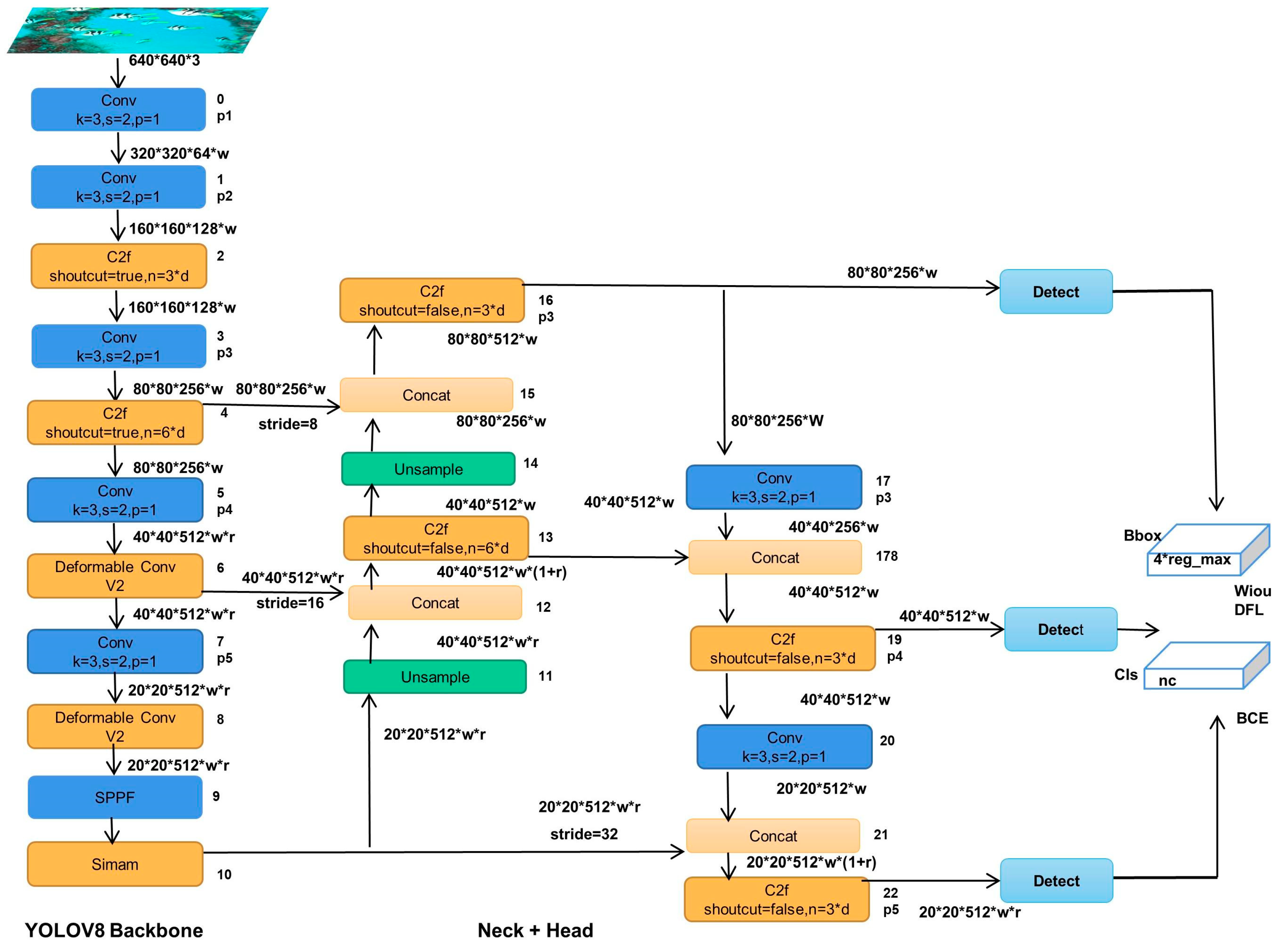
19] used Swin transform as the backbone network of yolov5, then, improved the PAnet multi-scale feature fusion method and confidence loss function, which effectively improved the object detection accuracy and the robustness of the model. In this paper, we improved the network structure of YOLOv8n, added a parameter-free attention mechanism, and finally optimized the loss function. The improved structure diagram is shown in
Figure 1.
2.2. Fusion of deformable convolutional feature extraction network
Deformable Convolution v2 [
20] is an improved version of Deformable Convolution v1 [
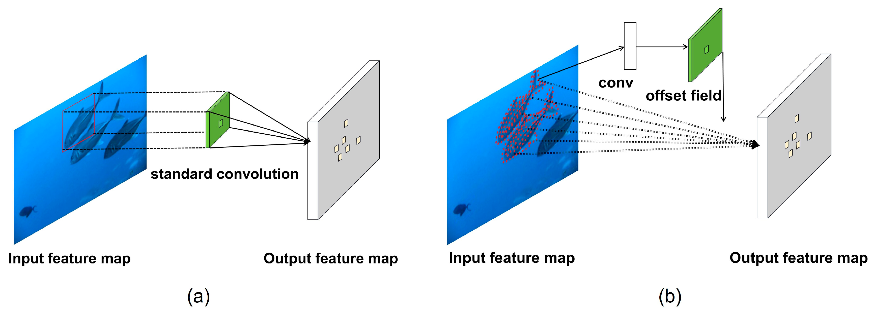
21], which further enhances and optimizes the previous method. In a common convolution module, fixed-size and shape convolution filters are used. However, during the feature extraction process, there may be interference where the convolution kernel does not align perfectly with the target region and includes excess background noise. In comparison, Deformable Convolution v2 introduces additional offsets, allowing the convolution operations to better align with the target region in the feature map. This enhancement in Deformable Convolution v2 provides improved modeling capabilities in two complementary forms. Firstly, it extends the use of deformable convolutional layers throughout the network. By incorporating more convolutional layers with adaptive learning, Deformable Convolution v2 can effectively control sampling across a wider range of feature levels. Secondly, an adjustment mechanism is introduced, which not only enables each sample to experience learning shifts but also adaptively adjusts the learning target feature amplitude.
Compared with traditional convolution modules, deformable convolution is superior to traditional convolution in feature extraction accuracy. In the network structure of YOLOv8, we adjusted some nodes in the network structure, and replaced C2f modules at positions 6 and 8 in the backbone network structure with Deformable Convnets V2 modules. The robustness of the model is effectively enhanced. The difference between common convolution module and deformable convolution v2 shown in
Figure 2.
The calculation formula for the output of the feature map obtained by the common convolution is shown in Equation (1).
The calculation formula of deformable convolution v2 is show in equation (2), where
is the actual position of the pixel in the feature map,
is the position of the convolution point relative to the convolution kernel.
and
in the formula that are obtained in the training of the network., where
and
in the formula represent the learnable offset and modulation range at the kth position. While
is a real number with unconstrained range. The range of
is [0,1]. So, we will get the
maybe a decimal. Bilinear interpolation will be used to change the number from a decimal to an integer.
2.3. Simple and efficient parameter-free attention mechanism
Attention mechanisms are widely applied in both computer vision and NLP. In particular, high-resolution image processing tasks often face information processing bottlenecks. Drawing inspiration from human perception processes, researchers have been exploring selective visual attention models. Currently, the main attention mechanisms include the channel attention mechanism and the spatial attention mechanism. The channel attention mechanism compresses global information and learns from each channel dimension. It assigns different weights to different channels using an incentive method. On the other hand, the spatial attention mechanism combines global information to process important parts, transforming various spatial data and automatically selecting the more important area feature. These two attention mechanisms represent the 1D and 2D attention mechanisms [
22,
25], respectively. Underwater target detection differs from conventional target detection due to its susceptibility to illumination changes. One contributing factor is the varying light intensity caused by different weather conditions and time. Then, light transmission in the water will be affected by water absorption, reflection and scattering and serious attenuation, which will directly lead to the underwater image visible range is limited, blurred, low contrast, color incongruity and background noise and other problems. In order to reduce the impact of the above situation. We added the SimAm attention mechanism [
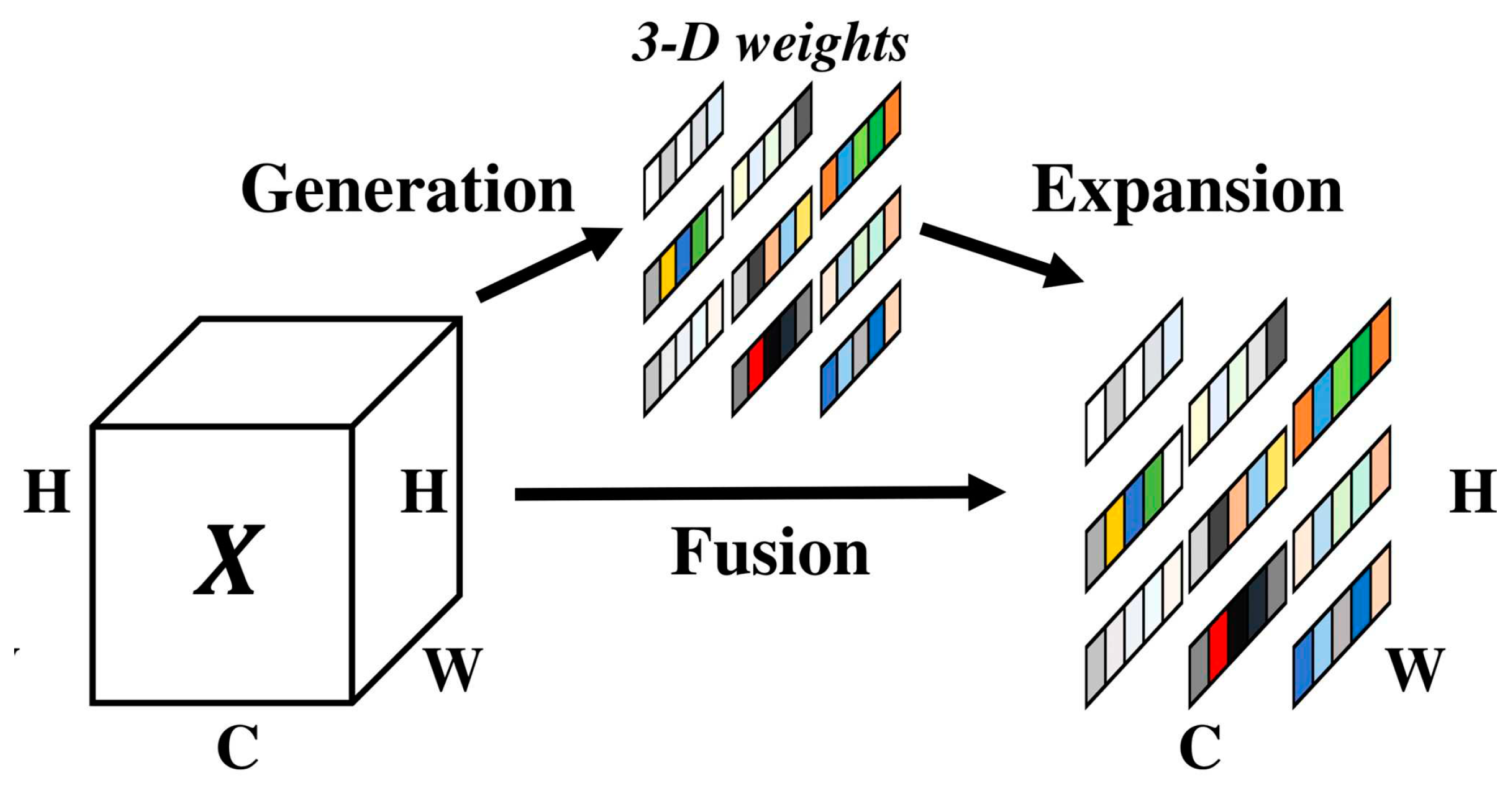
26] to backbone's layer 10. The parameter-free attention mechanism is simple and efficient. Most of the operators are selected based on the energy function, no additional adjustments to the internal network structure are required [
27]. The features with full 3D weights that showed in
Figure 3.
SimAm inspired from neuroscience theory, the parameter-free attention mechanism establishes the energy function in order to obtain the importance of each neuron. The calculation formulate is show in equation (3).
where
and
for the linear transformation of
and
, they represent neurons of a signal channel and other channel in the input feature map, respectively.
and
are the weights and biases after transformation. In order to simplify the formula, we use binary labels and add regular terms to the formula. We get a new definition of the energy function as follows the equations (4).
Theoretically, each channel has M energy functions, where M=H×W. However, iteratively solving this equation requires a lot of computational resources, we do a better optimization of the computation with
and
, which show in the equation (5)
where
and
is mean and variance of other neurons in the channel,
represents the regularization parameter. The existing solution in formula (5) is obtained on a single channel, so it is reasonable to assume that the pixels in the channel all follow the same distribution. So, we can calculate the mean and variance of all neurons and use it for all neurons on the channel. Since it takes a large amount of computing power resources to calculate μ and σ by iterative calculation, this method can reduce the computation amount well. Therefore, the calculation formula of minimum energy function show in equation (6).
If the result of
is lower, it means that the difference between neuron
and other neurons is more obvious, it also means that it’s more important. The importance of each neuron can be obtained by
. Our approach treats each neuron individually and integrates this linear separability into an end-to-end framework, as show in the equation (7).
where E groups all
across channels and dimensions, E is the energy function on each channel, in order to prevent the value of E from being too large. Using the sigmoid activation function to limit the value of E. SimAm can be flexibly and easily applied to other target object algorithms, integrating it into the backbone network of YOLOv8n, effectively refine the characteristics of the channel domain and spatial domain, thereby significantly improving the accuracy of object detection without increasing the complexity and computing resources of the network. [
29]
2.4. Loss function with dynamic focusing mechanism
The loss function is crucial for enhancing the model's performance. Traditional loss functions only consider the overlap between the predicted and ground truth bounding boxes, without taking into account the region between them. This limitation becomes problematic for small target detection, as the loss function cannot be differentiated if there is no intersection between the predicted and ground truth bounding boxes. Consequently, the network model cannot be optimized, leading to deviations in the evaluation results [
30,
31]. In the YOLOv8n network model, the Distribution Focal Loss and CIoU loss functions are employed as the loss functions. The CIoU loss function incorporates the loss of detection box scale and the loss of length and width ratio, in addition to the DIOU loss function. These enhancements contribute to improved accuracy in regression prediction. However, it is worth noting that the CIoU loss function requires more computational resources during model training within the original YOLOv8n network structure. Second, the datasets may contain low-quality data samples, which may contain other background noise, uncoordinated ratio of length to width and other geometric factors, which may further aggravate the negative impact of its training. That cannot eliminate the negative impact of geometric factors. So, we improve the above problem by using Wise-IoU [
32] to replace CIoU.
2.4.1. WIoU v1
Low quality datasets will inevitably have a negative impact on the model, which usually comes from geometric factors such as distance and aspect ratio, etc. Therefore, we construct WIoU v1 with two layers of attention based on the distance metric, as follows the equation (8) and (9) [
33].
where
∈ [1,e), which can significantly enlarge the
of the anchor box.
and
are the minimum width and height of the enclosing box. By separating
and
from the computed graph, gradients that hinder convergence can be prevented without introducing new conditions such as aspect ratio.
2.4.2. WIoU v2
WIoU v2 borrows the design method of Focal Loss to construct a monotonic focusing coefficient on the basis of WIoU v1. However, it also has another problem with the introduction of this monotonic focusing coefficient, which will cause the gradient change when the model is backpropagated. The gradient gain decrease with the decrease of
, which causes the model to take more time to converge at a later stage. Therefore, we take the mean of
as a normalization factor, which is a good way to speed up the later convergence of the model. Where
as the exponential running average with momentum [
34]
2.4.3. WIoU v3
The quality of the anchor box is reflected by defining an outlier value. High quality anchor box has smaller outliers value. Utilizing higher quality anchor box to match a smaller gradient gain, which can better focus the Bounding box regression frame more on the ordinary quality anchor box, and the small gradient gain can match the anchor frame with large outliers, which can better reduce the large harmful gradient produced by low-quality samples. Based on WiouV1, a non-monotonic focusing coefficient β is constructed, and the gradient gain is highest when the value of the β is constant C. Due to
: It is dynamic, so the quality evaluation criteria of the anchor box are also dynamic, which allows WiouV3 to dynamically adjust the gradient gain distribution strategy.
3. Experiments
3.1. Underwater target detection dataset
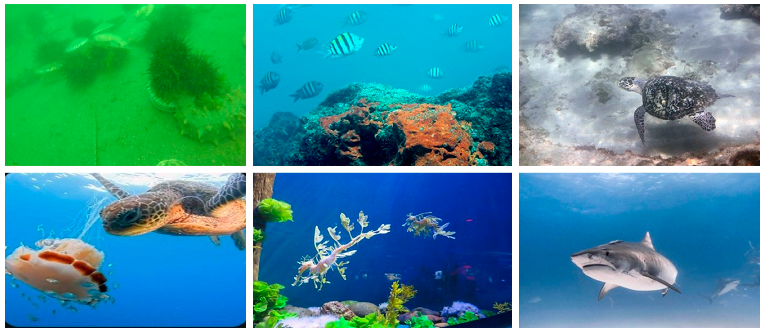
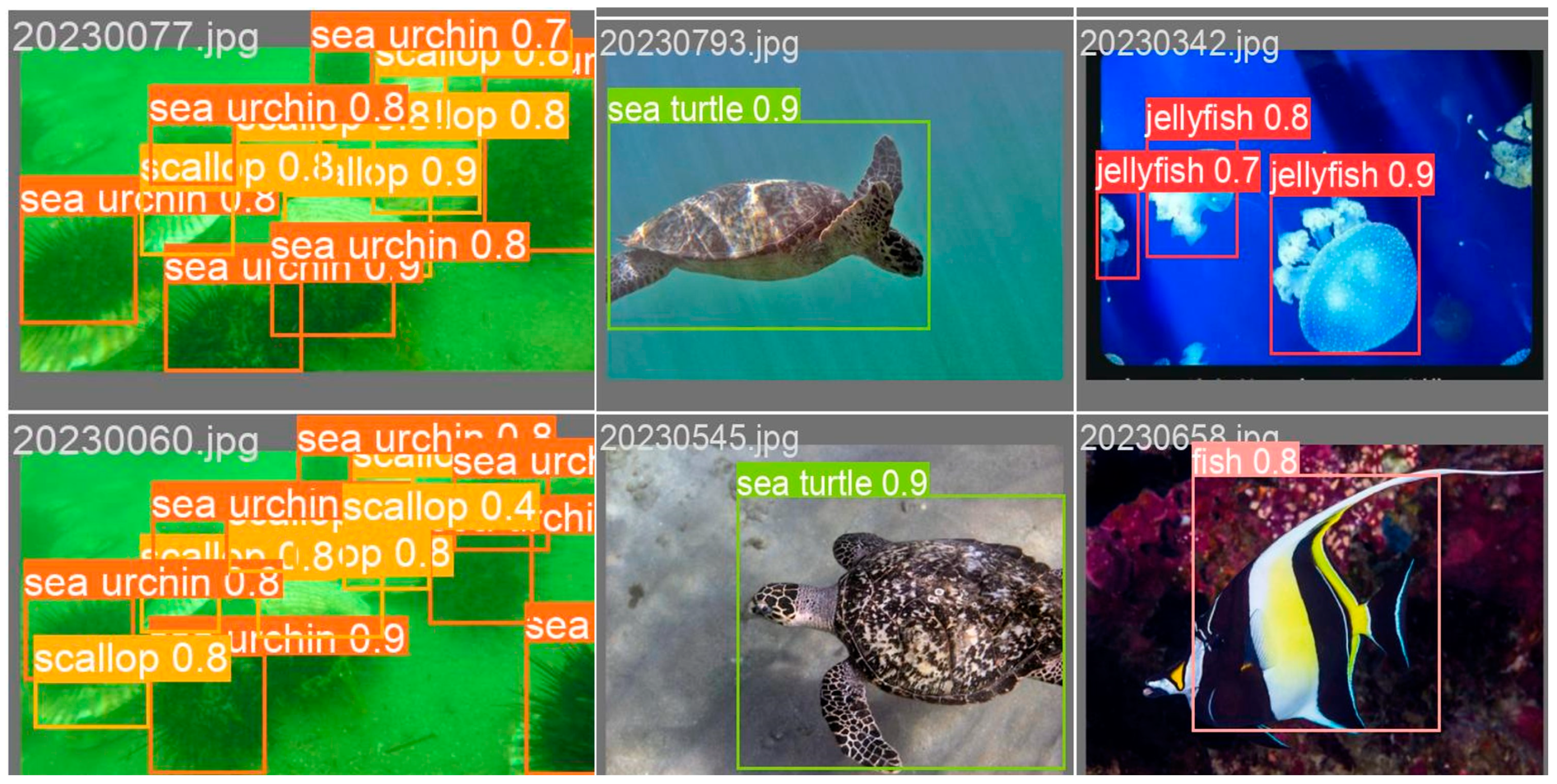
In this experiment, we validate our method using a self-constructed underwater target detection dataset and the Pascal VOC dataset. Our underwater target detection dataset consists of two parts: one part is obtained from the Target Recognition Group of China Underwater Robot Professional Competition (URPC), and the other part is collected from the publicly available dataset on the whale community platform. The dataset includes a total of seven categories, namely scallops, sea urchins, sea cucumbers, fish, turtles, jellyfish, sharks, and seagrass.
Figure 4 shows a portion of the underwater target detection dataset, which consists of 1585 images. All images in the dataset are annotated using the Labelimg software and are in yolo format. The dataset is randomly divided into training set, test set, and validation set in a ratio of 7:2:1.
Figure 5 provides an analysis of the dataset.
Figure 5a shows the number of instances for each category, while
Figure 5b presents the size and number of ground truth boxes in the target area. It can be observed that the dataset contains a relatively higher proportion of small targets. Where 5(c) and 5(d) analyze the center point and aspect ratio of the image label, respectively.
3.2. Experimental configuration and environment
The python programming language and pytorch deep learning framework were used in our experiment, and Ubuntu18.4 was used as the operating system. The hardware configuration is shown in
Table 1 below. The hyperparameter during training are as follows: the input size of the image is 640*640, the total Epoch of training is 200 times, the batch-size is 16, SGD is used to optimize the model, the initial learning rate is set to 0.01, the momentum is set to 0.973, and the weight attenuation is set to 0.0005. The training process uses the Mosaic data enhancement strategy.
3.3. Model evaluation metrics
we used recall rate, average detection time, average accuracy rate and the number of parameters of the model to evaluate the performance of the improved YOLOV8n model, in equations (12) and (13), TP and FP are the proportion of positive samples in the dataset that are correctly predicted and incorrectly predicted, and FN is the quantity of samples in the negative sample that are incorrectly predicted. While the recall rate increases, the accuracy maintains a higher value, indicating that the performance of our model is better.
In the formula (14), AP is the area under the accuracy and recall curves, and the larger the area obtained, the higher the accuracy of the model. mAP represents the average precision for each class, x denotes the number of classes in the dataset.
4. Analysis and discussion of experimental result
4.1. Comparsion of experimental results of different model
To demonstrate the superiority of the improved YOLOv8n, we conducted a comparative experimental study using the current mainstream target detection model. Specifically, we compared the performance of DAMO-YOLO, YOLOv7, YOLOX, and the original YOLOv8n models. The experimental results, as shown in
Table 2, include measurements such as Flops (number of floating-point operations per second) and params (number of model parameters). Additionally, we evaluated the average precision (mAP) at different IoU thresholds. The mAP@0.5 represents the average across all categories when the IoU threshold is set to 0.5, while mAP@0.5:0.95 represents the average mAP for each category at different thresholds ranging from 0.5 to 0.95 with a step size of 0.05.
In the comparison experiment, all models used default parameters, and the input image size for all models was set to 640x640. Notably, the improved YOLOv8n model exhibited a 3.2% increase in mAP@0.5 and a 4.1% increase in mAP@0.95 compared to the original model. Furthermore, the number of parameters in the improved model was reduced by 6.1%. When compared to other mainstream target detection algorithms, the mAP@0.5 of the improved YOLOv8n was found to be 8.3%, 10.3%, and 19% higher than that of YOLOv7, YOLOX, and DAMO-YOLO, respectively. Similarly, the mAP@0.95 of the improved YOLOv8n was 9.6%, 13.2%, and 18.7% higher than that of YOLOv7, YOLOX, and DAMO-YOLO, respectively. The number of parameters and floating-point computation of the model are better than other models.
4.2. Comparsion of ablation experimens
In the ablation experiment, we verified each module in the improved model and analyzed its effect on the model. Among them, the loss function selects the best WiouV3 for the ablation experiment. The results are shown in
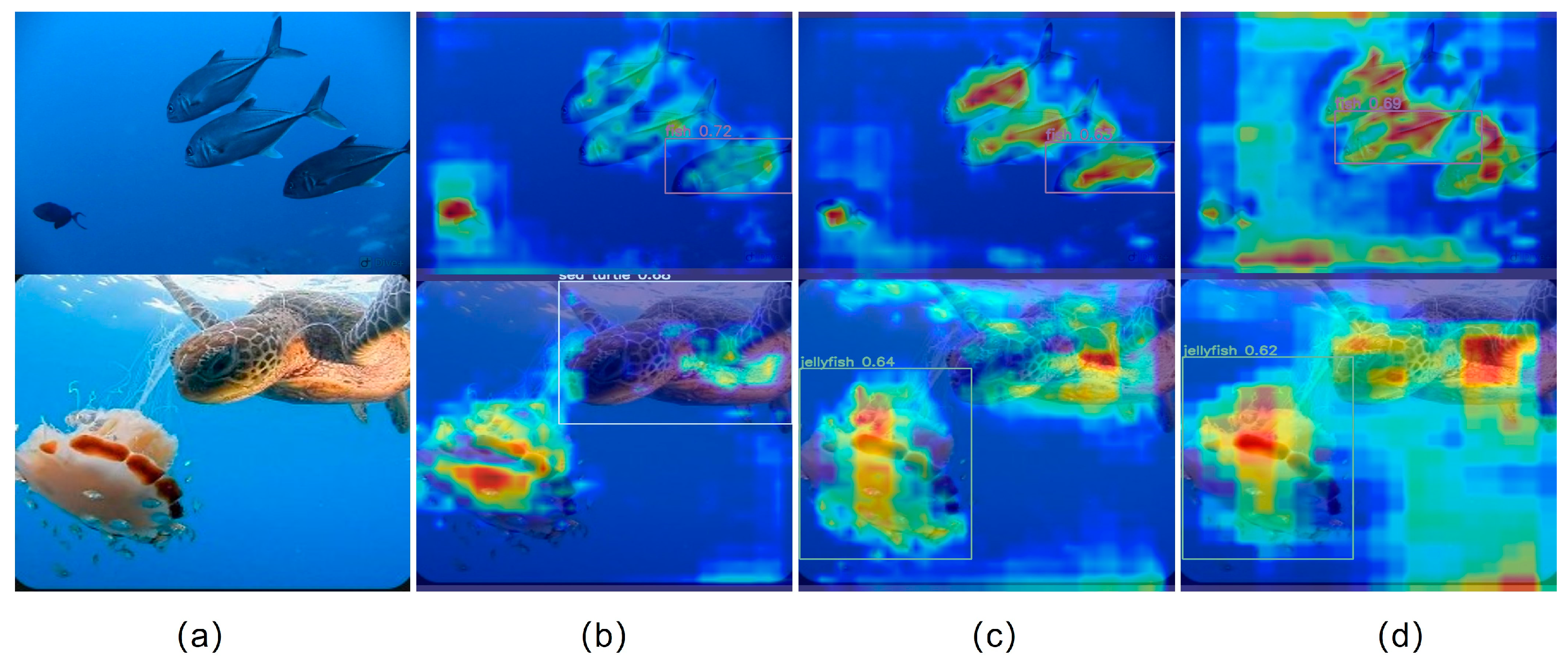
Table 3. From the experiment results, it can be observed that DefConv2, SimAm, and Wiouv3 have improved the mAP@0.5 accuracy of the model by 2.4%, 1.6%, and 3%, respectively. The mAP@0.5::0.95 also increased by 2.2%, 3.4%, and 2% respectively. When combined with DefConv2 and SimAm on the basis of WIoUv3, the accuracy of mAP@0.5 improved by 2.9% and 0.1%, respectively. The mAP@0.5::0.95 also increased by 2.5% and 3%, respectively. Overall, DefConv2 shows better improvement in the accuracy of model detection. To visually compare the effect before and after adding the SimAm module, we utilized the Grad-CAM [
35] image shown in
Figure 6.
Figure 6a represents the original input image,
Figure 6(b) shows the normal heat map output image,
Figure 6c displays the thermal image after passing through the SimAm module, and
Figure 6d presents the heat map output of the last layer of the backbone network. By comparing the thermal effect plots of
Figure 6b,c, it can be observed that the information of the target area becomes more prominent in the output image after adding the SimAm module. and the thermal effect will be more obvious.
In order to compare the improvement effect of different versions of Wise-IoU on the model, we conducted further ablation experiments on the loss function Wise-IoU. The experimental data are shown in
Table 4. On the basis of adding Defconv2 and SimAm to the model, Wiouv1, Wiouv2 and Wiouv3 were added respectively. The experimental results show that mAP@0.5 of Wiouv3 increases by 0.86% and 0.7%, mAP@0.5:0.95 by 0.1% and 0.6%, respectively, compared with Wiouv1 and Wiouv2. At the same time, the average detection speed of each image is decreased by 0.03ms and 1.9ms, respectively. Through the above comparative analysis, Wiouv3 can improve the effect of our model better.
4.3. Pascal VOC dataset experimental results
The PASCAL Visual Object Classes is an open world-class computer vision challenge. The dataset can be applied to classification, localization, detection, segmentation, and action recognition tasks. To validate our method further, we utilized the Pascal VOC dataset, which consists of 17,125 images across 20 categories. We used the public dataset that Pascal VOC2012 to further verify and analyze our model. Our experiment involved dividing the dataset into a training set (12,330 images), a test set (3,425 images), and a validation set (1,370 images), following a 7:2:1 ratio. The hyperparameters used during model training were consistent with those of the underwater target detection dataset. Due to the larger size of the Pascal voc2012 dataset and slower model convergence, we increased the number of epochs trained to 300. The detailed experimental results are presented in
Table 5, where the inclusion of the DefConv2, SimAm, and Wiouv3 modules led to improvements of 2.5%, 1.9%, and 1.3% respectively. This demonstrates that these three methods effectively enhance the detection accuracy. Additionally, when comparing the number of parameters in the model, the addition of DefConv2 resulted in a 4.8% reduction, while the inclusion of the SimAm module improved the detection accuracy and recall without altering the number of floating-point operations or parameters in the model. The effectiveness of Wiouv1, Wiouv2, and Wiouv3 on the model based on DefConv2 and SimAm was analyzed.
Table 5 shows that Wiouv3 achieved the highest detection accuracy, with mAP@0.5 and mAP@0.95 being 3.5% and 2.4% higher than the original model, respectively.
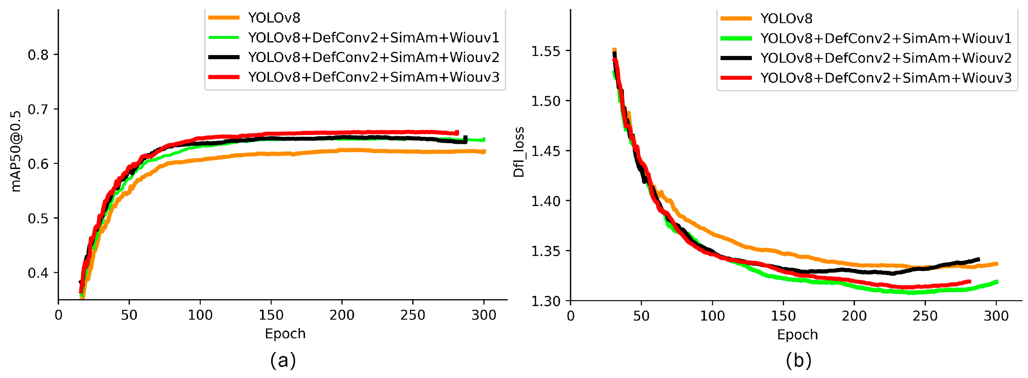
To visually observe the impact of the three versions of Wise-IoU on the model, we plotted the mAP@0.5 accuracy and DFL-loss curves in Figure 8. The red curve represents the performance after integrating DefConv2, SimAm, and Wiouv3, indicating that the model has reached an optimal state. Compared to Wiouv1, there was a 1.2% and 0.6% improvement, respectively, and a 1% improvement relative to Wiouv2. The experimental results on the Pascal voc2012 dataset align with the results of our own underwater target dataset, confirming the effectiveness of the proposed improvement method for YOLOv8n algorithm.
Figure 6.
mAP@0.5 precision changes are shown in (a); DFL-Loss curve changes are shown in (b).
Figure 6.
mAP@0.5 precision changes are shown in (a); DFL-Loss curve changes are shown in (b).
5. Conclusion
This paper addresses the challenges posed by poor underwater image quality, which hinder the extraction of feature information in the target area and result in missed detection of small targets. To overcome these issues, we propose three improvements to YOLOv8n. Firstly, we enhance the feature extraction capability of the backbone network by replacing the two-layer convolutional module with DefConv2. Secondly, we introduce a flexible and efficient SimAm module in the last layer of the backbone. The core idea behind SimAm is to assign attention weight vectors to different positions of the input feature map. Finally, we optimize the loss function by using the dynamic non-monotonically focused bounding box loss instead of the original CIoU. Through ablation experiments, we demonstrate that Wiouv3 outperforms Wiouv1 and Wiouv2 in terms of improvement effect, average detection speed, and detection accuracy of the model. The effectiveness of our method was validated by using the underwater target detection dataset and the Pascal VOC dataset. The results showed improved detection accuracy and a reduction in the number of parameters of the model. In future work, we aim to explore methods to effectively reduce the amount of floating-point computation in the model and develop a more lightweight object detection model.
Author Contributions
Q.L.: Conceptualization, Writing and Methodology. W.H.: Methodology and given the guidance. X.D and J.H.: Organize and label the dataset, Writing. Q.L, H.W, T.H, and J.Y.: performed the experiments. All authors have read and agreed to the published version of the manuscript.
Data Availability Statement
No applicated.
Conflicts of Interest
The authors declare no conflict of interest.
References
- Sun, Y.; Zheng, W.; Du, X.; Yan, Z. Underwater Small Target Detection Based on YOLOX Combined with MobileViT and Double Coordinate Attention. J. Mar. Sci. Eng. 2023, 11, 1178. [Google Scholar] [CrossRef]
- Wang, S.; Tian, W.; Geng, B.; Zhang, Z. Resource Constraints and Economic Growth: Empirical Analysis Based on Marine Field. Water 2023, 15, 727. [Google Scholar] [CrossRef]
- Wang, S.; Li, W.; Xing, L. A Review on Marine Economics and Management: How to Exploit the Ocean Well. Water 2022, 14, 2626. [Google Scholar] [CrossRef]
- Yuan, X.; Guo, L.; Luo, C.; Zhou, X.; Yu, C. A Survey of Target Detection and Recognition Methods in Underwater Turbid Areas. Appl. Sci. 2022, 12, 4898. [Google Scholar] [CrossRef]
- Zhang, C.; Zhang, G.; Li, H.; Liu, H.; Tan, J.; Xue, X. Underwater target detection algorithm based on improved YOLOv4 with SemiDSConv and FIoU loss function. Front. Mar. Sci. 2023, 10, 1153416. [Google Scholar] [CrossRef]
- Lei, Z.; Lei, X.; Zhou, C.; Qing, L.; Zhang, Q. Compressed Sensing Multiscale Sample Entropy Feature Extraction Method for Underwater Target Radiation Noise. IEEE Access 2022, 10, 77688–77694. [Google Scholar] [CrossRef]
- Li, W.; Zhang, Z.; Jin, B.; Yu, W. A Real-Time Fish Target Detection Algorithm Based on Improved YOLOv5. J. Mar. Sci. Eng. 2023, 11, 572. [Google Scholar] [CrossRef]
- Redmon, J.; Divvala, S.; Girshick, R.; Farhadi, A. 2016. You only look once: Unified, real-time object detection. In: Proceedings of the IEEE conference on computer vision and pattern recognition. pp: 779-788.
- Redmon, J.; Farhadi, A. 2017. Yolo9000: Better, faster, stronger. In: Proceedings of the IEEE conference on computer vision and pattern recognition. pp: 7263-7271.
- Bochkovskiy, A.; Wang, C.-Y.; Liao, H.-Y.M. Yolov4: Optimal speed and accuracy of object detection. arXiv 2020, arXiv:2004.10934. [Google Scholar]
- Terven, J.; Cordova-Esparza, D. A comprehensive review of yolo: From yolov1 to yolov8 and beyond. arXiv 2023, arXiv:2304.00501. [Google Scholar]
- Li, C.; Li, L.; Jiang, H.; Weng, K.; Geng, Y.; Li, L.; Ke, Z.; Li, Q.; Cheng, M.; Nie, W. Yolov6: A single-stage object detection framework for industrial applications. arXiv 2022, arXiv:2209.02976. [Google Scholar]
- Wang, C.-Y.; Bochkovskiy, A.; Liao, H.-Y.M. Yolov7: Trainable bag-of-freebies sets new state-of-the-art for real-time object detectors. In: Proceedings of the IEEE/CVF Conference on Computer Vision and Pattern Recognition. pp. 7464–7475. [CrossRef]
- Ge, Z.; Liu, S.; Wang, F.; Li, Z.; Sun, J. Yolox: Exceeding yolo series in 2021. arXiv 2021, arXiv:2107.08430. [Google Scholar]
- Xu, X.; Jiang, Y.; Chen, W.; Huang, Y.; Zhang, Y.; Sun, X. Damo-yolo: A report on real-time object detection design. arXiv 2022, arXiv:2211.15444. [Google Scholar]
- Zheng, Z.; Wang, P.; Liu, W.; Li, J.; Ye, R.; Ren, D. 2020. Distance-iou loss: Faster and better learning for bounding box regression. In: Proceedings of the AAAI conference on artificial intelligence. pp: 12993-13000.
- Lou, H.; Duan, X.; Guo, J.; Liu, H.; Gu, J.; Bi, L.; Chen, H. DC-YOLOv8: Small-Size Object Detection Algorithm Based on Camera Sensor. Electronics 2023, 12, 2323. [Google Scholar] [CrossRef]
- Zhang, J.; Chen, H.; Yan, X.; Zhou, K.; Zhang, J.; Zhang, Y.; Jiang, H.; Shao, B. An Improved YOLOv5 Underwater Detector Based on an Attention Mechanism and Multi-Branch Reparameterization Module. Electronics 2023, 12, 2597. [Google Scholar] [CrossRef]
- Lei, F.; Tang, F.; Li, S. Underwater Target Detection Algorithm Based on Improved YOLOv5. J. Mar. Sci. Eng. 2022, 10, 310. [Google Scholar] [CrossRef]
- Zhu, X.; Hu, H.; Lin, S.; Dai, J. 2019. Deformable convnets v2: More deformable, better results. In: Proceedings of the IEEE/CVF conference on computer vision and pattern recognition. pp: 9308-9316.
- Dai, J.; Qi, H.; Xiong, Y.; Li, Y.; Zhang, G.; Hu, H.; Wei, Y. 2017. Deformable convolutional networks. In: Proceedings of the IEEE international conference on computer vision. pp: 764-773.
- Guo, M.-H.; Xu, T.-X.; Liu, J.-J.; Liu, Z.-N.; Jiang, P.-T.; Mu, T.-J.; Zhang, S.-H.; Martin, R.R.; Cheng, M.-M.; Hu, S.-M. Attention mechanisms in computer vision: A survey. Comput. Vis. Media 2022, 8, 331–368. [Google Scholar] [CrossRef]
- Woo, S.; Park, J.; Lee, J.-Y.; Kweon, I.S. 2018. Cbam: Convolutional block attention module. In: Proceedings of the European conference on computer vision (ECCV). pp: 3-19.
- Hu, J.; Shen, L.; Sun, G. 2018. Squeeze-and-excitation networks. In: Proceedings of the IEEE conference on computer vision and pattern recognition. pp: 7132-7141.
- Wang, Q.; Wu, B.; Zhu, P.; Li, P.; Zuo, W.; Hu, Q. 2020. Eca-net: Efficient channel attention for deep convolutional neural networks. In: Proceedings of the IEEE/CVF conference on computer vision and pattern recognition. pp: 11534-11542.
- Lai, Y.; Ma, R.; Chen, Y.; Wan, T.; Jiao, R.; He, H. A Pineapple Target Detection Method in a Field Environment Based on Improved YOLOv7. Appl. Sci. 2023, 13, 2691. [Google Scholar] [CrossRef]
- Dong, C.; Cai, C.; Chen, S.; Xu, H.; Yang, L.; Ji, J.; Huang, S.; Hung, I.-K.; Weng, Y.; Lou, X. Crown Width Extraction of Metasequoia glyptostroboides Using Improved YOLOv7 Based on UAV Images. Drones 2023, 7, 336. [Google Scholar] [CrossRef]
- Yang, L.; Zhang, R.-Y.; Li, L.; Xie, X. 2021. Simam: A simple, parameter-free attention module for convolutional neural networks. In: International conference on machine learning. PMLR: pp: 11863-11874.
- Mao, R.; Wang, Z.; Li, F.; Zhou, J.; Chen, Y.; Hu, X. GSEYOLOX-s: An Improved Lightweight Network for Identifying the Severity of Wheat Fusarium Head Blight. Agronomy 2023, 13, 242. [Google Scholar] [CrossRef]
- Rezatofighi, H.; Tsoi, N.; Gwak, J.; Sadeghian, A.; Reid, I.; Savarese, S. 2019. Generalized intersection over union: A metric and a loss for bounding box regression. In: Proceedings of the IEEE/CVF conference on computer vision and pattern recognition. pp: 658-666.
- Zhang, Y.-F.; Ren, W.; Zhang, Z.; Jia, Z.; Wang, L.; Tan, T. Focal and efficient IOU loss for accurate bounding box regression. Neurocomputing 2022, 506, 146–157. [Google Scholar] [CrossRef]
- Tong, Z.; Chen, Y.; Xu, Z.; Yu, R. Wise-iou: Bounding box regression loss with dynamic focusing mechanism. arXiv 2023, arXiv:2301.10051. [Google Scholar]
- Zhu, Q.; Ma, K.; Wang, Z.; Shi, P. YOLOv7-CSAW for maritime target detection. Front. Neurorobotics 2023, 17, 1210470. [Google Scholar] [CrossRef] [PubMed]
- Zhao, Q.; Wei, H.; Zhai, X. Improving Tire Specification Character Recognition in the YOLOv5 Network. Appl. Sci. 2023, 13, 7310. [Google Scholar] [CrossRef]
- Selvaraju, R.R.; Cogswell, M.; Das, A.; Vedantam, R.; Parikh, D.; Batra, D. Grad-CAM: Visual Explanations from Deep Networks via Gradient-Based Localization. In Proceedings of the 2017 IEEE International Conference on Computer Vision (ICCV), Venice, Italy, 22–29 October 2017; pp. 618–626. [Google Scholar] [CrossRef]
|
Disclaimer/Publisher’s Note: The statements, opinions and data contained in all publications are solely those of the individual author(s) and contributor(s) and not of MDPI and/or the editor(s). MDPI and/or the editor(s) disclaim responsibility for any injury to people or property resulting from any ideas, methods, instructions or products referred to in the content. |
© 2023 by the authors. Licensee MDPI, Basel, Switzerland. This article is an open access article distributed under the terms and conditions of the Creative Commons Attribution (CC BY) license (http://creativecommons.org/licenses/by/4.0/).
