Efficient Cumulant-Based Automatic Modulation Classification Using Machine Learning

Preprint

Article

Efficient Cumulant-Based Automatic Modulation Classification Using Machine Learning

Altmetrics

Downloads

135

Views

Comments

A peer-reviewed article of this preprint also exists.

Ben Dgani^*,

Israel Cohen^*

Ben Dgani^*,

Israel Cohen^*

This version is not peer-reviewed

Submitted:

24 August 2023

Posted:

25 August 2023

You are already at the latest version

Alerts

Abstract

This paper presents a novel method for automatic modulation classification (AMC) for cognitive radio (CR) networks based on a simple classifier that is trained with high-order cumulant. The proposed method focuses on the statistical behavior of modulated signals and includes analog modulation and digital schemes, which received less attention in the literature. The effectiveness of the proposed method is demonstrated through simulation results using high-quality generated signals under different signal-to-noise ratios (SNRs) and channel conditions. The classification performance achieved by the proposed method is superior to that of the more complex deep learning methods, making it well-suited for deployment in end units of CR networks, particularly in military and emergency service applications. The proposed method offers a cost-effective, high-quality solution for AMC that meets the stringent requirements of these critical applications.

Keywords:

Subject: Engineering - Electrical and Electronic Engineering

1. Introduction

The modern era of radio communication is often associated with smart transmitters, adaptive receivers, and an overall intelligent communication network, taking advantage of modern technologies to improve and optimize our usage of wireless channels. One important task when implementing intelligent radio modulation detection for the received signal. Automatic modulation classification is an intermediate step between signal detection and demodulation, which plays a vital role in various civilian and military applications, which are varied and usually massive. Said networks have been active for years with an established network structure for wireless communication. Both civil and military networks require fast and adaptive radio networks to combat various tasks daily and in times of need. For this purpose, we consider the SDR platform.

Software Defined Radio (SDR) is a platform for radio communication where its communication functions are realized as a software program instead of the traditional hardware components. The programmable radio functions allow the SDR to be adaptive and dynamic for different networks and tasks. The SDR is the modern realization of the “software radio” term, which was coined by Mitola [1]. The conversion of the signal processing to the digital domain allows SDR-based networks to include complex algorithms that improve communication rate, accuracy, and even distance. One typical example is Cognitive Radio, where an SDR program can perform spectrum sensing and spectrum management tasks instead of using expensive and overly complex hardware, even if possible. Cognitive radio was introduced in 1999 by Mitola [2]. The idea behind CR is to develop a programmable radio unit that can dynamically and automatically manage its communication network using the software. CR function as a solution to the spectral congestion problem in the current age of communication, where the number of daily users is constantly increasing, and the spectrum resources become more expensive and sparser. The CR can adapt to its environment and set up an unlicensed communication network that shares the same wireless spectrum with another user. The unlicensed users in this scenario are mainly the military and emergency services, which might need immediate response to any crisis and can get the government authority to abuse the shared spectrum without any interruptions. Setting up the shared network includes a method called spectrum sensing.

In the spectrum sensing step, the cognitive radio scans the available channels for parameters and finds ’empty holes,’ unused frequencies in the spectrum. The channel parameters sensing works into the adaptive qualities of CR and allows units to dynamically change the modulation scheme used for transmission to improve rates and quality. The dynamic modulations mean the spectrum sensing function must have a recognition method of the received signal modulation scheme. This method is known as Automatic Modulation Classification, which may also appear in literature as modulation recognition and modulation detection [3,4,5].

Automatic Modulation Classification is the process of detecting and identifying the unknown modulation scheme of a radio signal, dating back to the 1980s [6,7] but gained more popularity after the publication of the Cognitive Radio idea. The modern AMC literature is focused on deep learning and neural networks; the classic AMC algorithms are split between two methods [8]. The first set of methods are the likelihood-based algorithms which are accurate but require high computational complexity. This can be a significant setback when discussing fast and efficient radio systems while limiting the types of usable SDR models for implementation only to the most expensive ones. This high cost can be troublesome for the mentioned services as both are mostly government funded and relies on cost-efficient projects.

The second set of methods is feature-based (FB). The FB algorithms extract classification features from the signal, such as high order statistical moments (HOS) or instantaneous frequency and phase parameters [9]. After the algorithm extracts the features, they are used for classification. Such algorithms include support vector machines, decision trees, and K-means. In recent years, thanks to the massive growth in the field of neural networks, most novel studies regarding AMC involve using neural networks, either for feature extraction, the classification process, or both. The neural networks algorithm has optimal results in terms of classification accuracy, reaching high detection probability at a low SNR value. Like the likelihood-based methods, neural networks can suffer from high computational complexity. They might take a large amount of system storage if a deep network model is used. The mentioned disadvantages can be a significant problem when dealing with a quick setup radio network that relies on end units and requires both power and time efficiency.

In this paper, we focus on the FB method for the AMC, where the key features we use are the high-order cumulants (HOCs). Cumulants are alternatives to statistical moments, such as mean and variance. The HOCs are popular in AMC literature as a detection feature [10,11]. This can be attributed to their additive property that separates the desired signal from its additive noise, which will be explained further in this paper. Most of the literature discusses digital modulation classification [12,13]. However, this novel work aims to include analog modulations as well. In this paper, we study the statistics of eleven modulation schemes, explore the best classification feature for each modulation, and discover the statistical connection between pairs of modulations.

The rest of this paper is organized as follows. Section 2 presents the modulated signal models, the theory behind HOS, and cumulants. In Section 3, we evaluate the simulation results for our proposed FB method. Finally, in Section 4, we discuss the conclusions from the results.

2. Materials and Methods

We divided the following section into three subsections. The first part includes a brief review of the theory of high-order statistics and the cumulants, an alternative for the more familiar moments. The second part introduces the dataset we used for our work. The last subsection explains the theoretical part of the classification process.

2.1. High Order Statistics

In statistics, moments of a random variable provide quantitative measures related to the shape of its probability density graph and the distribution behavior. Specifically, the nth order moment of a random variable x is defined by

m_{n} (x) = \int x^{n} f (x) d x,

(1)

where

f (x)

is the probability density function of x. If the nth order moment integral diverges, the nth order moment of the variable does not exist. If the nth order moment of x exists, so does the

(n - 1)

th order moment, and thus all lower order moments. We define a central moment by

m_{n} (x - μ)

, which is the mean value of x, and define the normalized moment as

m_{n} (x / σ)

where

σ

is the standard deviation.

The cumulants

c_{n}

of a probability distribution are an alternative to the moments of the distribution. Any two probability distributions whose moments are identical will also have identical cumulants, and vice versa. The first, second, and third cumulants are the same as the central moments, but fourth and higher-order cumulants are not equal to central moments. The cumulant of a random variable x is defined using the cumulant-generating function

C_{t} (x) = l o g (E [e^{t x}]),

(2)

and the cumulants

c_{n}

are obtained from a power series expansion of the cumulant generating function:

C_{t} (x) = \sum c_{n} \frac{t^{n}}{n!} .

(3)

Since this expansion is a Maclaurin series, the nth-order cumulant is obtained by differentiating the expansion n times at t=0. The use of cumulants instead of moments in the literature is based on their cumulative property: assume X and Y are independent random variables, then

c_{n} (X + Y) = c_{n} (X) + c_{n} (Y) .

(4)

The cumulant generating function can be challenging to calculate. However, we can use the moments to calculate the cumulants based on [11,14]. We use

\begin{matrix} c_{4, 0} & = & m_{4, 0} - 3 m_{2, 0}^{2} \end{matrix}

(5)

\begin{matrix} c_{4, 1} & = & m_{4, 1} - 3 m_{2, 1} m_{2, 0} \end{matrix}

(6)

\begin{matrix} c_{4, 2} & = & m_{4, 2} - {| m_{2, 0} |}^{2} - 2 m_{2, 1}^{2} \end{matrix}

(7)

\begin{matrix} c_{6, 0} & = & m_{6, 0} - 15 m_{4, 0} m_{2, 0} + 30 m_{2, 0}^{3} \end{matrix}

(8)

\begin{matrix} c_{6, 3} & = & m_{6, 3} - 9 c_{4, 2} m_{2, 1} - 6 m_{2, 1}^{2} \end{matrix}

(9)

\begin{matrix} c_{8, 0} & = & m_{8, 0} - 28 m_{6, 0} m_{2, 0} - 35 m_{4, 2}^{2} + 420 m_{4, 0} m_{2, 0}^{2} - 630 m_{2, 0}^{4} \end{matrix}

(10)

. where

m_{q, p}

is the mixed moment

E (x^{q} * {\bar{x}}^{p - q})

. This set of equations enables simple and fast calculation for the HOC, which will act as features for the classification algorithm. The classification method in our paper uses the cumulants above as input features, along with the matching cumulants

C_{p, q} (x_{d})

for the derivative of the signal

x_{d} [n] = x [n + 1] - x [n] .

(11)

After experimenting with different features, we added the cumulants of the derivative to the features list, including separated cumulants for the real and imaginary parts of the signal and the cumulants of the amplitude and phase of each signal. Only the derivative’s cumulants have noticeably improved the classification accuracy.

The main advantage of working with cumulants appears when discussing AWGN. The noise is a random process that follows a normal distribution, therefore we can use its cumulant generating function, which is calculated in [15,16] using

C_{t} (w) = l o g (M_{t} (w)) = μ t + σ^{2} \frac{t^{2}}{2},

(12)

where

μ

and

σ

are the mean and standard deviation, respectively. The function in (12) is a second-order polynomial, so its 3rd and higher-order derivatives are zero-valued, meaning the HOC cumulants of AWGN are equal to zero. Hence, The HOC of the sum between AWGN and another independent random process will equal the HOC of the second random process alone. Since the derivative of AWGN is distributed the same, the derivative’s cumulants are still effective for our method under the above assumptions.

2.2. Modulation and Signal Model

The signals used in this paper are taken from the RadioML2018.01A dataset [17]. This dataset contains 2,555,904 frames. Each frame is 1024 IQ samples from a modulated signal, with various modulation schemes and SNR values from

- 20

to 30 dB. The dataset contains 24 different modulations generated using SDR under the following channel specification:

Selective multipath Rician fading;
Carrier frequency offset;
Symbol rate offset;
Non-impulsive delay spread;
Doppler shift;
AWGN.

We only consider 11 modulations considered the “Normal” set. This includes the following: OOK, 4ASK, BPSK, QPSK, 8PSK, 16QAM, AM-SSB-SC, AM-DSB-SC, FM, GMSK, OQPSK. (We will refer to AM-SSB-SC and AM-DSB-SC as SSB and DSB, respectively). We decided to evaluate our work on the “Normal” dataset since it is considered the benchmark for classification models in the literature, in contrast to the “hard” set, which contains all 24 schemes.

2.3. Decision Tree

A decision tree is a flowchart-like model for supervised learning in which each internal node represents a decision test on a single feature, each branch represents the outcome of the test, and each leaf node represents a class label. The paths from root to leaf represent classification rules. Decision trees have several advantages as a classification model, and we are focusing on two of them in this paper. The first is that training the tree model does not require a large dataset; this is a significant advantage over neural networks that are widely popular in the literature despite the need for massive data to yield results. The second advantage is the model’s simplicity, which allows it to combine with other decision techniques. The benefit of combining techniques comes when we make a tree model, where instead of a simple decision rule at each node, we can use a more complex model.

The decision tree model we used in our work is from the Python scikit-learn (Sklearn) library, which is trained based on Gini impurity. Gini impurity is a measurement for the probability of classifying the labels incorrectly. Let A be a random variable that takes one of k labels

(a_{1}, a_{2}, . . . a_{k}

); then we define the Gini impurity of a classification model as

G (A) = 1 - \sum_{i = 1}^{k} {(P (a_{i}))}^{2} .

(13)

The training process of a decision tree contains three steps:

Decide feature to split the data: for each feature, the Gini impurity is calculated, and the one for which it is minimized is selected;
Continue splitting the data based on 1;
Stop splitting the data if we reach a certain tree depth.

The Decision tree model’s parameters are the comparison threshold at each node, barring the leaves, meaning the total number of parameters in a tree of depth d can be calculated with

P_{n} = 2^{H} - 1,

(14)

this is also the number of calculations a single tree applies when classifying since there is no need for multiplications or additions.

3. Results

The suggested classification method requires hand-picked features for each step, so we start the simulation with a small-scale experiment. We use a simple decision tree to classify all 11 labels in a single model, each time using only a single feature from the entire list. Table 1 shows the results of this experiment.

We only pick the best two features for the following simulations for every modulation. The next part of the simulation is picking the training set for the model. Usually, machine learning algorithms randomly pick train sets from the entire data. However, we consider only a subset of the data in this case. Where SNR is higher than a certain threshold. Modulated signals have a minimal SNR requirement for perfect demodulation. Classification Accuracy at negative SNR is irrelevant for most labels since even if the signal is detected, it cannot be adequately demodulated. So, we split the data into two groups, high SNR and low SNR, and try to pick an SNR threshold for the splitting. 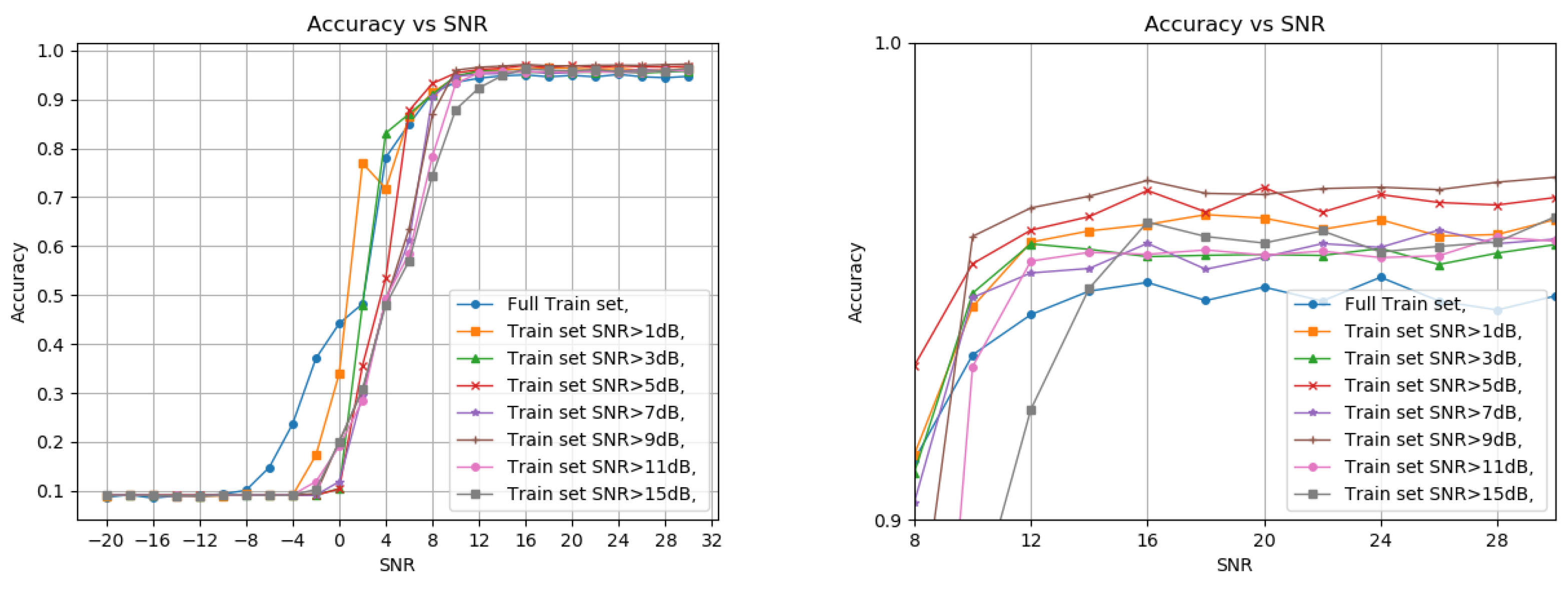Figure 1 shows the classification results for the train set split under different SNR thresholds, including a zoom-in on the highest accuracy section.

First, picking a train set from all the SNR values gives better results at negative SNR but deteriorates when reaching a positive value, as expected. Another conclusion is that using over 5 dB as the threshold gives lesser accuracy for high and low SNR test samples. The final choice of threshold was between 1 dB and 5 dB. While the 1 dB threshold provides better accuracy at lower SNR, starting from 4 dB and higher, we get a slight improvement in detection accuracy for the 5 dB threshold. This result supports the assumption that modulation schemes have minimal SNR requirements for perfect demodulation. The depth of the decision tree was not considered for the first test. So, we want to pick a balanced tree, deep enough to view all the features we chose before while not too deep, which can result in overfitting and high complexity.

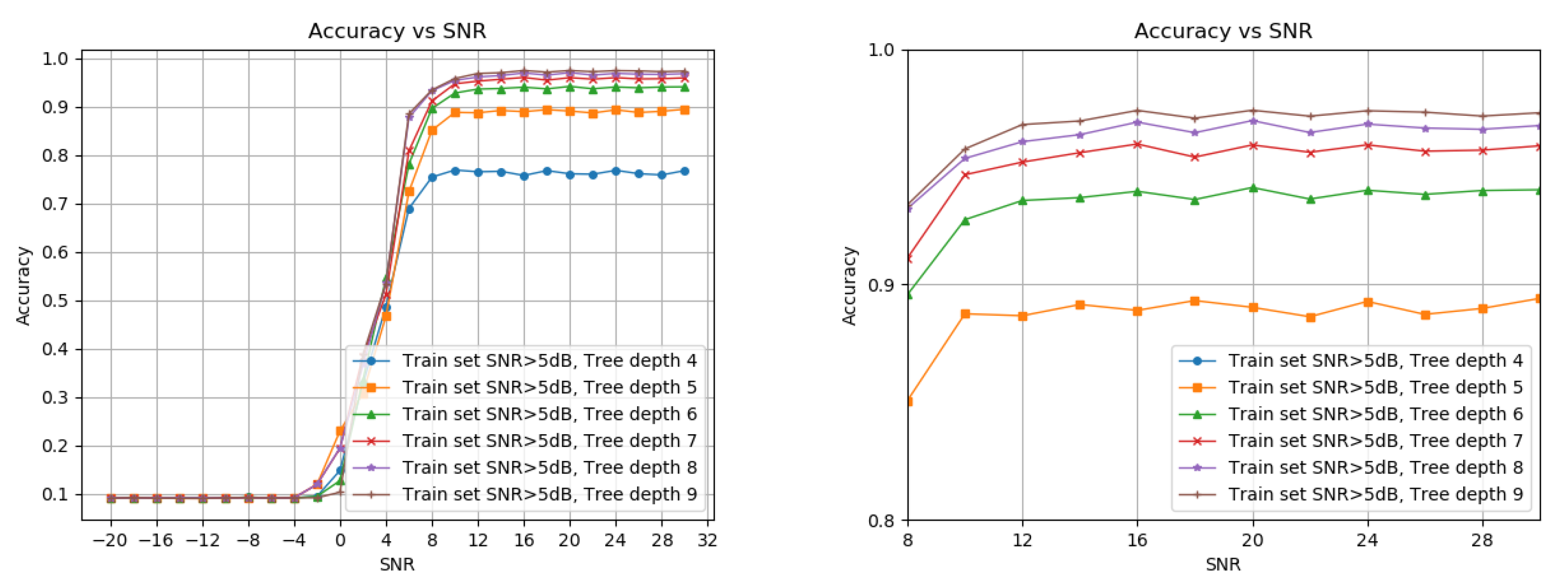
Figure 2 shows the detection probability under different decision tree depths. We start at four layers, since this is the minimal depth for 11 labels, and stops at nine as we see no significant improvement from 8. The optimal depth for each application can be chosen based on memory and runtime requirements. We picked an 8-deep tree with a higher than 5 dB SNR train set.

4. Discussion

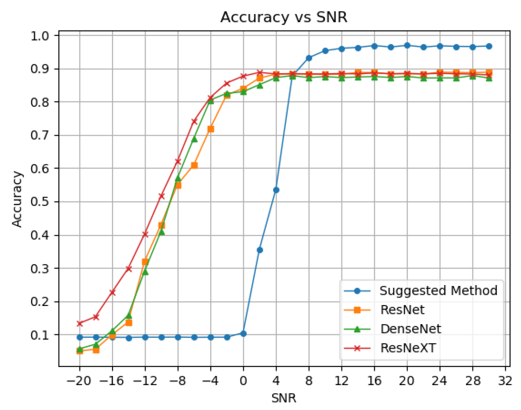
We aim to compare our results to state-of-the-art deep learning models. First, we take inspiration from Hao Zhang et al. [18] who compare their method with three different models of deep neural networks. The models we examine are ResNet [19], DenseNet [20] and ReNeXT [21]. We aim to compare our model to the neural networks in two manners. Figure 3 shows the first comparison of neural networks in the classification accuracy.

We can see the advantage of deep neural networks in the negate SNR zone, while our method fails in comparison. However, we have already discussed why classification at negative SNR is usually irrelevant in terms of perfect demodulation. Starting from the splitting threshold of 6 dB SNR, our suggested method yields better detection accuracy than the popular NN methods by a margin of almost 8%.

The second comparison with the NN models is the parameters or memory requirement. We use (14) to calculate the total parameters needed for different tree depths and compare them in Table 2 with the proposed NN models. Our model, even with an addition of layers, can reach a few hundred or thousands of parameters, while the NN models reach millions. The sparse memory use can be beneficial when considering adding a few models together for improved accuracy and when the desire for low complexity and short runtime is critical.

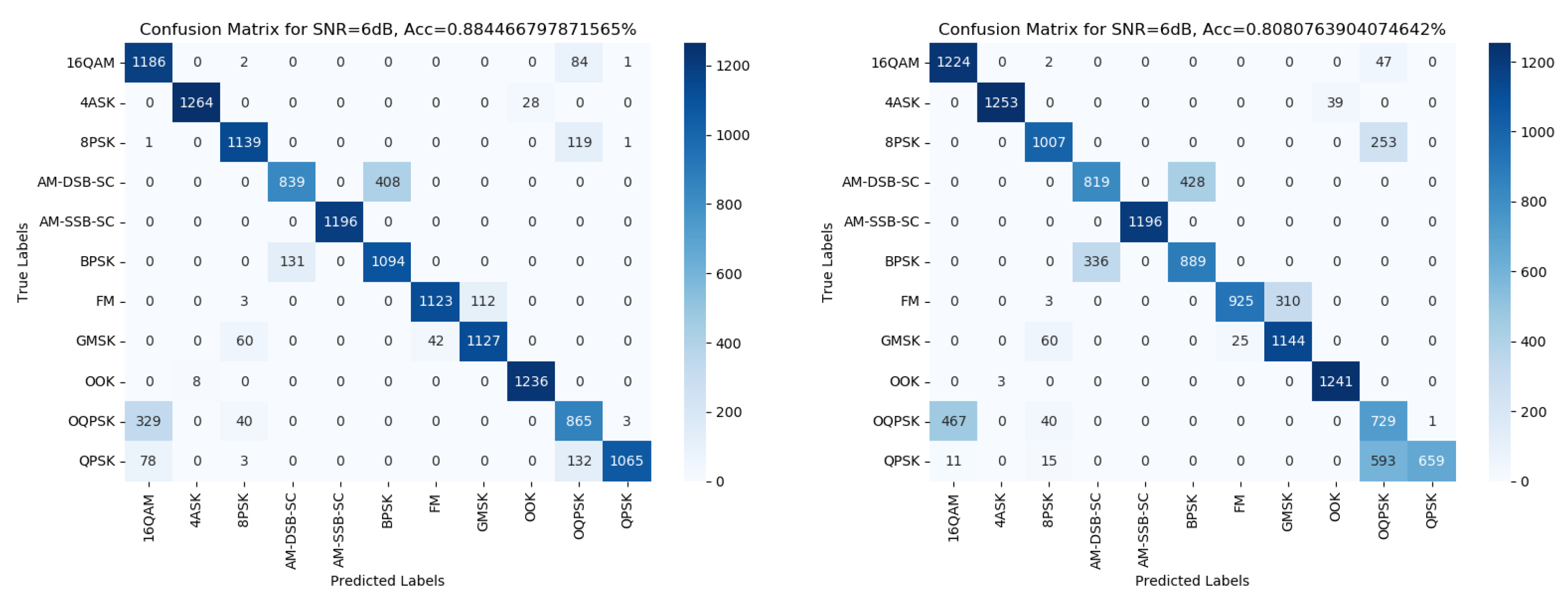
We examine the confusion matrix from the suggested method. Figure 4 shows the confusion matrices at 6 dB for the 7 and 8 deep decision trees under the 5 dB SNR threshold train set. We observe in the illustrated figures, as well as in other matrices we examined, that the mislabeling of the model is consistent – meaning the labels that can get mismatched are almost always the same. Based on this observation, we can split the modulation schemes into subgroups as follows:

Group 0 - AM-SSB;
Group 1 - AM-DSB and BPSK;
Group 2 - 4ASK and OOK;
Group 3 - FM and GMSK;
Group 4 - 8PSK, 16QAM, QPSK and OQPSK.

Group 0 contains only SSB as it is almost instantly detectable using nearly every feature, starting from positive SNR value and under every model we tried. Groups 1, 2, and 3 are pairs of modulations that get mixed up commonly at lower SNR, leading us to assume that the signal model of their schemes is statistically similar. Group 4 is more significant and includes the rest of the modulations that get mixed up with one another without any pair being more common than the other.

5. Conclusions

Our work considered a simple model for automatic modulation classification for spectrum sensing. The suggested method is superior to some of the widely popular neural networks in terms of accuracy and memory. The decision tree classifier was chosen for this paper based on its simplicity. It gives us the benefit of learning which statistical features, in the form of HOC, are efficient for which modulation scheme. The research also explored the viability of cumulants in classifying analog modulations in addition to digital, which most cumulants-based works tend to ignore. After learning the identifying cumulants for each modulation, we also observed subgroups of modulation with similar statistical behavior, which opened directions for better classification methods. The minimal parameters and high accuracy allow our method to be considered optimal for end units in CR networks, where memory and speed efficiency are essential. In future work, we will explore how the modulation subgroups can be used to build a more complex method with improved accuracy while also trying to adapt our method to the more extensive set of modulations.

Funding

This research received no extrernal funding.

Institutional Review Board Statement

Not applicable.

Informed Consent Statement

Not applicable.

Data Availability Statement

This research is based on the published dataset by Timothy James O’Shea; Tamoghna Roy and T. Charles Clancy. Available at https://www.deepsig.ai/datasets.

Acknowledgments

Not applicable.

Conflicts of Interest

The authors declare no conflict of intesert.

Abbreviations

The following abbreviations are used in this manuscript:

AMC	Automatic modulation Classification
CR	Cognitive radio
SDR	Software defined radio
SNR	Signal to Noise Ratio
FB	Feature based
HOS	High order statistical moments
HOC	High order cumulants
AWGN	Additive white Gaussian noise

References

Mitola, J. (1995). The software radio architecture. IEEE Communications magazine, 33(5), 26–38. [CrossRef]
Mitola, J., and Maguire, G. Q. (1999). Cognitive radio: making software radios more personal. IEEE personal communications, 6(4), 13–18. [CrossRef]
Haque, M., Sugiura, Y., and Shimamura, T. (2019). Spectrum Sensing Based on Higher Order Statistics for OFDM Systems over Multipath Fading Channels in Cognitive Radio. Journal of Signal Processing, 23(6), 257–266. [CrossRef]
Bozovic, R., and Simic, M. (2019). Spectrum Sensing Based on Higher Order Cumulants and Kurtosis Statistics Tests in Cognitive Radio. Radioengineering, 29(2). [CrossRef]
Salahdine, F. (2017). Spectrum sensing techniques for cognitive radio networks. arXiv preprint arXiv:1710.02668. [CrossRef]
Callaghan, T. G., Perry, J. L., and Tjho, J. K. (1985). Sampling and algorithms aid modulation recognition. Microwaves, 24, 117–119.
Nebabin, V. G., and Sergeev, V. V. (1984). Methods and techniques of radar recognition. Moscow Izdatel Radio Sviaz.
Dobre, O. A., Abdi, A., Bar-Ness, Y., and Su, W. (2007). Survey of automatic modulation classification techniques: classical approaches and new trends. IET communications, 1(2), 137–156. [CrossRef]
Hazza, A., Shoaib, M., Alshebeili, S. A., and Fahad, A. (2013, February). An overview of feature-based methods for digital modulation classification. In 2013 1st international conference on communications, signal processing, and their applications (ICCSPA) (pp. 1–6). IEEE. [CrossRef]
Sun, X., Su, S., Zuo, Z., Guo, X., and Tan, X. (2020). Modulation classification using compressed sensing and decision tree–support vector machine in cognitive radio systems. Sensors, 20(5), 1438. [CrossRef]
Shih, P., and Chang, D. C. (2011, August). An automatic modulation classification technique using high-order statistics for multipath fading channels. In 2011 11th international conference on ITS telecommunications (pp. 691–695). IEEE. [CrossRef]
Hazza, A., Shoaib, M., Alshebeili, S. A., and Fahad, A. (2013, February). An overview of feature-based methods for digital modulation classification. In 2013 1st international conference on communications, signal processing, and their applications (ICCSPA) (pp. 1–6). IEEE. [CrossRef]
Swami, A., and Sadler, B. M. (2000). Hierarchical digital modulation classification using cumulants. IEEE Transactions on communications, 48(3), 416–429. [CrossRef]
Jdid, B., Lim, W. H., Dayoub, I., Hassan, K., and Juhari, M. R. B. M. (2021). Robust automatic modulation recognition through joint contribution of hand-crafted and contextual features. IEEE Access, 9, 104530–104546. [CrossRef]
Fryntov, A. E. (1989). Characterization of a Gaussian distribution by gaps in its sequence of cumulants. Theory of Probability and Its Applications, 33(4), 638–644. [CrossRef]
Volkmer, H. (2014). A characterization of the normal distribution. J. Stat. Theory Appl., 13(1), 83–85. [CrossRef]
O’Shea, T. J., Roy, T., and Clancy, T. C. (2018). Over-the-air deep learning based radio signal classification. IEEE Journal of Selected Topics in Signal Processing, 12(1), 168–179. [CrossRef]
Zhang, H., Wang, Y., Xu, L., Gulliver, T. A., and Cao, C. (2020). Automatic modulation classification using a deep multi-stream neural network. IEEE Access, 8, 43888–43897. [CrossRef]
Zhang, K., Zuo, W., Chen, Y., Meng, D., and Zhang, L. (2017). Beyond a gaussian denoiser: Residual learning of deep cnn for image denoising. IEEE transactions on image processing, 26(7), 3142–3155. [CrossRef]
Huang, G., Liu, Z., Van Der Maaten, L., and Weinberger, K. Q. (2017). Densely connected convolutional networks. In Proceedings of the IEEE conference on computer vision and pattern recognition (pp. 4700–4708). [CrossRef]
Xie, S., Girshick, R., Dollár, P., Tu, Z., and He, K. (2017). Aggregated residual transformations for deep neural networks. In Proceedings of the IEEE conference on computer vision and pattern recognition (pp. 1492–1500). [CrossRef]

Figure 1.

P_{d}

based on train set SNR threshold. (a) Full view; (b) Zoomed in view.

Figure 1.

P_{d}

based on train set SNR threshold. (a) Full view; (b) Zoomed in view.

Figure 2.

P_{d}

based on tree depth. (a) Full view; (b) Zoomed in view.

Figure 2.

P_{d}

based on tree depth. (a) Full view; (b) Zoomed in view.

Figure 3.

P_{d}

comparison for the suggested method.

Figure 3.

P_{d}

comparison for the suggested method.

Figure 4. Confusion Matrices for different tree depth: (a) depth=7; (b) depth=8.

Table 1. Best two features for each modulation at SNR=10dB.

Modulation	1st Feature	$P_{d}$	2nd Feature	$P_{d}$
SSB	$C_{4, 1}$	100%	$C_{4, 0}$	100%
DSB	$C_{4, 1}^{d}$	74.69%	$C_{4, 0}^{d}$	73.34%
BPSK	$C_{2, 0}$	99.57%	$C_{4, 0}$	92.73%
FM	$C_{4, 1}$	99.63%	$C_{2, 0}$	99.27%
GMSK	$C_{4, 2}$	96.09%	$C_{8, 0}$	81.23%
OOK	$C_{2, 0}$	95.82%	$C_{2, 1}$	93.61%
4ASK	$C_{2, 1}$	95.84%	$C_{2, 0}$	93.71%
QPSK	$C_{4, 0}^{d}$	87.95%	$C_{8, 0}^{d}$	86.69%
OQPSK	$C_{4, 2}$	76.39%	$C_{4, 0}$	60.53%
16QAM	$C_{6, 0}^{d}$	100%	$C_{6, 3}^{d}$	99.74%
8PSK	$C_{4, 0}^{d}$	100%	$C_{4, 2}^{d}$	99.87%

Table 2. Parameter size of different models.

Model	Total Parameters
6 Deep Tree	63
7 Deep Tree	127
8 Deep Tree	255
ResNet	16,805,830
DenseNet	2,658,310
ReNeXT	5,671,872

Disclaimer/Publisher’s Note: The statements, opinions and data contained in all publications are solely those of the individual author(s) and contributor(s) and not of MDPI and/or the editor(s). MDPI and/or the editor(s) disclaim responsibility for any injury to people or property resulting from any ideas, methods, instructions or products referred to in the content.

© 2023 by the authors. Licensee MDPI, Basel, Switzerland. This article is an open access article distributed under the terms and conditions of the Creative Commons Attribution (CC BY) license (http://creativecommons.org/licenses/by/4.0/).

Copyright: This open access article is published under a Creative Commons CC BY 4.0 license, which permit the free download, distribution, and reuse, provided that the author and preprint are cited in any reuse.

MDPI Initiatives

Important Links

Choose an area of interest and we will send you notifications of new preprints at your preferred frequency.

Disclaimer

Efficient Cumulant-Based Automatic Modulation Classification Using Machine Learning

Abstract

1. Introduction

2. Materials and Methods

2.1. High Order Statistics

2.2. Modulation and Signal Model

2.3. Decision Tree

3. Results

4. Discussion

5. Conclusions

Funding

Institutional Review Board Statement

Informed Consent Statement

Data Availability Statement

Acknowledgments

Conflicts of Interest

Abbreviations

References

MDPI Initiatives

Important Links

Subscribe